Segmentation of wood cell in cross-section using deep convolutional neural networks

Abstract

Fiber and vessel structures located in the cross-section are anatomical features that play an important role in identifying tree species. In order to determine the microscopic anatomical structure of these cell types, each cell must be accurately segmented. In this study, a segmentation method is proposed for wood cell images based on deep convolutional neural networks. The network, which was developed by combining two-stage CNN structures, was trained using the Adam optimization algorithm. For evaluation, the method was compared with SegNet and U-Net architectures, trained with the same dataset. The losses in these models trained were compared using IoU (Intersection over Union), accuracy, and BF-score measurements on the test data. The automatic identification of the cells in the wood images obtained using a microscope will provide a fast, inexpensive, and reliable tool for those working in this field.

Keywords

Image segmentation fiber-vessel microscopic wood cells deep convolutional neural networks

1 Introduction

As a safe, easy to handle, and aesthetic structure, woods have been used as building and engineering material since ancient times. Wooden materials are preferred mainly for their anatomical and chemical structures as well as their mechanical and physical properties. The rational use of this raw material is associated with the known structural properties of wood.

Anatomical features such as fibers, vessels, parenchyma, and rays play an important role in identifying wood species [1, 2]. These anatomical features affect the parameters related to the quality of wood and its area of use. Therefore, for the anatomical description of the microscopic character of each wood cell, the cells must be segmented accurately.

So far, numerous methods have been implemented for the segmentation of an image into groups of similar attributes, for determining the object class of each pixel [3, 4]. Yet, continuous improvement is necessary due to the need for more accurate techniques in this field. In recent years, deep learning has attracted the attention of researchers due to the need for more accurate and effective methods. The deep learning technique is used in various fields for better performance. It’s a preferred technique, especially in medical image analysis [5 –7]. Deep learning models, U-Net in particular, are very effective in image segmentation [8 –11].

In this regard, several studies were carried out using computer-aided analysis for the microscopic wood images. In most of these studies, the anatomical structures of the plants were analyzed using image processing [12]. For example, the watershed algorithm has been used to identify cells in the microscopic images of softwood [13, 14]. Another study has focused on the detailed analysis of the wood cell type, and addressed only three cell types: trachea, tracheid, and rays, the main cells of wood, which have been analyzed using image analysis software, and, height, sphericity, thickness, lumen and surface area of the cells have been calculated for each cell [15].

In another study, it was stated that two challenges need to be solved in pore segmentation. The first is the variety in sizes and shapes. Fibers and vessels are similar in color and shape but vary in size. Therefore, this variance should be considered to increase the accuracy of segmentation. Consequently, an algorithm based on mathematical morphology was proposed for the solution to this problem. This algorithm uses a disk-shaped structure element that changes its radius according to the porosity size [16].

The purpose of a segmentation network is to tag each pixel in an image in such a way that pixels with the same tag share certain properties. A segmentation network classifies each pixel in an image and provides an image segmented according to its class. Commonly used for image segmentation, the CNNs replace fully connected layers with convoluted layers to perform tagging each pixel. Such architectures consist of down-sampling and sampling steps, also known as encoders and decoders, respectively. However, additional sampling layers often provide more trainable parameters in such architectures [17 –20].

SegNet, which is used since 2015, is a practical, fully deep-convolutional neural network (CNN) architecture for semantic pixel-based segmentation. It consists of an encoder network, a corresponding decoder network, and a pixel-classification layer [21]. In the subsequent research, fully connected layers were removed to preserve high-resolution feature maps at the deepest encoder output. The excessive number of parameters is also significantly reduced in the SegNet encoder. Hence, SegNet provides significant improvements in accuracy, especially for smaller classes [18 –20]. Another study shows that the benefit of a significantly reduced number of parameters reduces memory consumption and feature extraction time, without compromising on the performance [22].

One of the popular approaches in segmentation is the use of an encoder-decoder structure. In the traditional autoencoder architecture, the size of the input information is reduced through the subsequent layers, starting with the first stage [23].The decoder part comes after the encoder of the architecture. Linear feature representation is learned in this part, and the size gradually increases. The output size at the end of the architecture is the same as the input size. The architecture is ideal for maintaining the output size, but as a drawback, it compresses the input linearly, resulting in a bottleneck that cannot covey all the features. It differs from the U-Net in this regard. The U-Net model performs deconvolution on the decoder side, and overcomes this “bottleneck” drawback, thanks to the connections from the encoder side of the architecture.

Although numerous studies have been conducted on the microscopic images of wood, studies with deep learning on wood cell images are still in their infancy [8, 24]. Vessel and fiber structures are very similar but vary in size according to the species. In traditional methods, especially in morphological-based image processing techniques, some parameters of each image must be changed or adjusted according to the size of the pore. Moreover, fibers and vessels are difficult to characterize in detail due to their multicellular structures. Therefore, a two-stage CNN structure, customized according to the characteristics of these cells, was proposed for the segmentation of the fiber and vessel cells. In this way, pores with similar shapes, but with different sizes were better identified. Since they contain sufficient information, a deep learning method was applied on smaller input image sizes, without the need for advanced hardware. The steps taken for the segmentation of wood images are discussed following sub-sections.

2 Material and methods

2.1 Preparation of the dataset

In the study, cross-section microscopic images of diffuse and semi-ring porous wood species were used [25]. The species include of Populus, Aesculus, Alnus Glutinosa, Aesculus Hippocastanum L. Juglans Acer, and Betula.

The images were labeled using morphological procedures [26]. The values of the structural elements to be selected can vary for each image. Thus, these elements need to be checked and identified for each image. After labeling, the images were controlled in line with expert guidance for an accurate wood image classification. The images were grouped under three classes: black for the background, white for fiber, and dark gray for woodgrain. Manual segmentation is one of the best methods for the segmentation of small datasets, but it’s a time-consuming process [27]. Figure 1 shows the original image and the corresponding labeling (ground truth).

Fig. 1

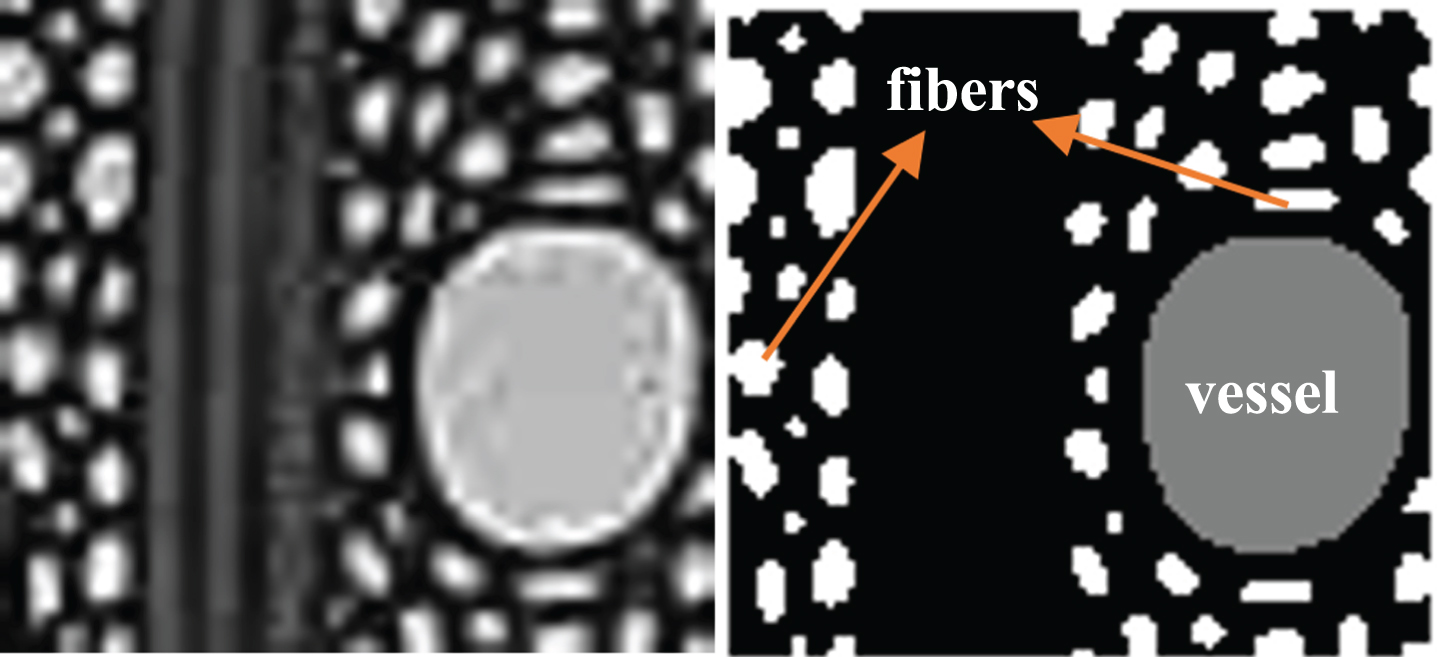
Original image and corresponding labeled image. (background (0), white for fiber and dark gray for vessel).

The original image was divided into patches of 48x48 pixel in size (Fig. 2). Of these 48x48-pixel patches, images with dominant background information were not taken into account and not included in the database. The database consists of 40000 patches of 48x48 pixels in size. After dividing the dataset into two parts as training and test sets (4000), data augmentation was performed. The training set was doubled using the data augmentation.

Fig. 2

Taking 48x48 non-overlapping patches, a) original image, b) Traning Patch Extraction.

Data augmentation is the most widely used method to increase the number of images in a dataset, improve the model”s performance, and reduce the over-adaptation in the image data. As adopted by numerous studies, data augmentation is an effective way of increasing training data set for deep learning [28 –30]. Data augmentation aims to help the network to learn features better. Rotation, translation, adding noise, reflection and contrast adjustment are among the frequently used methods of data augmentation in the literature.

The data were augmented by applying rotation, salt-and-pepper noise (0.01 to 0.05), circular mean filter (pillbox) for focus blur, gauss filter, reflection, and applying random transformations. Pillbox was used for simulating distortion seen in microscopic images.

There are three labeled classes in the dataset in this study. Since some classes may outperform the others in number, which may affect potential feature distributions and classification results, each class was weighted by the class balance method [31]. ${weight}_{i} = f_{i median} / f_{i}$ (1)

Where f_i _median is the median of all f_i; f_i is the pixel frequencies of class i.

Data class imbalance is a major problem negatively affecting especially minority classes in controlled classifiers. A wide variety of strategies have been developed to overcome this repetitive problem, including excessive sampling, sampling, preservation of natural proportions in training samples, data synthesis and class-weighted loss functions [32, 33].

2.2 Proposed method

In this study, a method is proposed for the segmentation of microscopic images of wood cross-sections. As shown in Fig. 3, the proposed method consists of a combination of two-stage CNN architectures.

Fig. 3

The architecture of the customized CNN model.

The first stage is composed of 3×3 filtered convolution layer with 64 channels, batch normalization (BN), and ReLU blocks. The convolution layer consists of a large number of trainable filters that can be updated during training. Filters apply the convolution process to the images coming from the previous layer and generate the output data. The activation map (feature map) is generated as a result of this convolution process. The activation map shows the regions with specific features discovered by each filter [34].

Then, the activation map is fed to the next layer. Padding is selected so that the output size of the convolution layer becomes equal to the input size. A BN layer normalizes each input channel along a mini-size. Batch normalization layers are often used between convolution layers and ReLU layers in order to speed up the training of CNNs and reduce the sensitivity to the initial condition of the network. The layer normalizes the activation of each channel by first calculating the mini-batch average and dividing it to the mini-batch standard deviation. Consequently, BN adds two trainable parameters to each layer, so the normalized output is multiplied by a gamma parameter and add a beta parameter [35]. $\hat{x_{i}} = \frac{x_{i} - μ B}{\sqrt{σ_{B}^{2} + ɛ}},$ (2) $y_{i} = γ \hat{x_{i}} + β \equiv {BN}_{γ, β} (x_{i})$ (3)

B = {x_1….m}: values of x over a mini-batch, ɛis a constant for numerical stability (very small). γ and β are parameters to learn and shift.

ReLU activation was added after all the convolutional and batch normalization layers in the network. $R (x) = max (0, x)$ (4)

As an effect on the input data, it sets negative values to zero. With the use of this layer, the network learns faster. ReLU is a non-linear and computationally simple method for capturing more complex properties of input data, and greatly accelerates CNN training [28, 30]. For most purposes, ReLU units are effective [36].

Unlike typical encoder-decoder based segmentation architectures, the image resolution is preserved from input to output of the first CNN. Therefore, the padding process is not necessary to maintain intermediate sizes of the images since we do not perform down-sampling on the image. Although sub-sampling (pooling) increases the robustness of a model against small variations in input, the image resolution will be poor in such cases. Since the maximum pooling process cannot be reversed, the pooling layer was not used for the images we use to prevent smoothing out small, porous features. Pooling is usually placed after the ReLU layer. Its main purpose is to reduce the input size for the next convolution layer. The reduction in size results in a loss of information due to this layer. Although the depth of the CNN architecture can be increased by additional layers, each additional layer will cause an extra parameter for training.

The second stage has an encoder-decoder architecture. The convolutional layer consists of BN, ReLU, and maximum pooling layers. The deconvolutional layer has upsampling, convolution, and BN layers. The maximum pooling layer divides the input into rectangular pooling regions and calculates the maximum of each region. $\begin{matrix} From feature map c \\ = {c_{1}, c_{2}, \dots c_{n - h + 1}} \\ \in ℝ^{n - h + 1}, \\ \hat{c} = max {c} \end{matrix}$ (5)

Although the pooling layer causes loss of information, it is useful for two reasons: It has a less computational burden for the following layers of the network, and reduces variance.

In the final stage, the feature maps obtained were sent to the softmax layer on a parallel network. Separate softmax classifiers were used for calculating the loss $σ {(x)}_{i} = \frac{e^{x_{i}}}{\sum_{j = 1}^{N} e^{x_{j}}}$ (6)

Where N is the number of classes, x is the input vector, and σ(x)i is the output class probability.

The class probabilities of each pixel are combined and sent to another softmax classifier. The output produces a segmented image at the same resolution as the input image.

2.3 Network training

Training is an iterative process, in which training data are fed into the model in groups, predictions are made with a forward-propagation by the current model, and errors between the predictions and labels in the accuracy table are calculated. Errors are back-propagated over the network, parameters (weights) are calculated for all neurons, and the parameters are updated to minimize errors [37].

The input weights are initialized with the Glorot initializer. The choice of initializer has a bigger impact on networks without batch normalization layers [38].

During learning, the loss function calculates the difference between the pixel class distributions and the predicted probabilities. $\begin{matrix} Loss (X) = - \sum_{i = 1}^{N} m_{i} logS (x_{i}) + \\ (1 - m_{i}) log (1 - S (x_{i})), for N classes \end{matrix}$ (7)

where m_i is truth value and x_i is the Softmax probability for the ith class.

The weights are updated at each mini-batch and a revised model is produced at each epoch. Adam (adaptive moment estimation) adaptive learning optimization algorithm was used to minimize loss Adam maintains an element-wise moving average of both the parameter gradients and their squared values. If the gradients contain too much noise, the moving average of the gradient becomes smaller, and therefore the parameter updates are smaller too [39].

The network was trained using the Adam optimization algorithm. The architecture of the first CNN consists of blocks 3×3 convolution with 64 channels. The learning rate was set to 0.0002, the mini-batch size was 4, the training period was 20, the basic learning rate was 0.001, momentum was 0.9 and gamma was 0.1. The learning rate was reduced by 0.1 times in every 5 epochs that of the previous one.

The patches are applied to first CNN and a probability map of the same size as the input image is obtained as output. This map shows the probability of the class to which each pixel belongs. There is no pooling layer at this stage. The output of the first layer was able to detect wood cells with relatively high sensitivity, but there were some problems in the border areas of the regions. In addition, it was planned to further improve the segmentation map in the first stage by applying the second stage.

The feature maps obtained are sent to the softmax layer on the parallel network. Separate softmax classifiers were used to calculate the loss. The class probabilities of each pixel are combined and sent to another softmax classifier. The result of the softmax function shows the probability of each category. As the last step of the proposed segmentation algorithm, the probability map obtained for wood cells is converted into a segmentation mask. The output produces a segmented image at the same resolution as the input image.

2.4 Evaluation metrics

Accuracy is the ratio of correctly classified pixels to the total number of pixels in that class, relative to the ground-truth, for each class. In other words, $Accuracy score = \frac{TP}{TP + FN}$ (8)

Global Accuracy is the ratio of correctly classified pixels, regardless of class, to the total number of pixels. $Global Accuracy = \frac{TP + TN}{TP + TN + FP + FN}$ (9)

where, true positives (TP), false positives (FP), false negatives (FN) and TN (true negative).

The IoU of two sets A and B (also known as Jaccard similarity coefficient) is expressed as; Jaccard(A,B)=| intersection(A,B) | / | union(A,B) |. The Jaccard index is related to the Dice index. In other words, $\begin{matrix} IoU = Jaccard (A, B) = \frac{TP}{TP + FP + FN} \\ = \frac{dice (A, B)}{2 - dice (A, B)} \end{matrix}$ (10)

The BF-score indicates how well the projected boundary of each class is aligned with the actual boundary. $BF score = \frac{2 * recision * recall}{recall + precision},$ (11) $\begin{matrix} where, \\ precision = \frac{TP}{TP + FP}, \\ recall = \frac{TP}{TP + FN} \end{matrix}$ (12)

3 Experimental results

In this study, a method is proposed for the automatic segmentation of wood cell images using deep neural networks. A 5-fold cross-validation data split was used for training in the proposed network. The sample segmentation results for test images are shown in Fig. 4. The segmentation results are indicated by the color scale for a more specific representation.

Fig. 4

Example segmentation results. a) test images, b) segmentation results with the proposed method (colored representation).

The pixels on the border region are added symmetrically around the image for the seamless segmentation of larger images by an overlap-tile strategy [17]. Even if 48x48 patches were used in training, the recommended method can be applied to the entire image.

To evaluate the method, it was compared with SegNet [20] and U-Net [17] architectures trained using the same dataset. The U-Net and SegNet architectures have often been used in literature as references in segmentation studies. The losses of the trained models were evaluated on the test data and the results were compared with ground truth. Since there was no previous study with this dataset, IoU, accuracy, and F-Score measurements were used to evaluate the segmentation results. A comparison of the segmentation methods is shown in Table 1. The values in the table show the average values of the test data for 5-fold validation.

Table 1

Numerical comparison of segmentation methods

	Global Acc	Mean Accuracy	Mean IoU	Weighted IoU	Mean BFScore
SegNet	0.711	0.722	0.563	0.562	0.437
U-Net	0.809	0.866	0.696	0.676	0.493
Proposed method	0.896	0.911	0.800	0.790	0.639

The global accuracy presented in Table 1 refers to the ratio of correctly classified pixels to the total number of pixels, regardless of class. Mean Accuracy refers to the mean accuracy of all classes in all images in the dataset. Mean IoU and BFScore are the average IoU and BF scores of all classes in all images, respectively. Weighted-IoU is the average IoU of each class, weighted by the number of pixels in that class. The values in Table 1 are the averages of test images. In this study, accuracies were 71% with SegNet, 80% with U-Net, and 89% with the proposed method, respectively. The proposed method was found to yield better results than the others.

4 Discussion

In order to identify a tree microscopically, it is necessary to determine the anatomical features of all individual cell types (vessels, axis and ray parenchyma, and fibers) in three cross-sections. Determining the features of each cell type depends on the precise segmentation of each cell into segments. The features of elements in images are key to identifying sample species. However, there are many difficulties in pore detection due to various challenges, such as varying shapes and sizes, ambiguous borders, and low image quality.

The quest for more accurate and effective methods, and the increase in the number of complex problems have led researchers to deep learning. Although large data sets are needed for the training process in the convolutional deep learning models, better results have been obtained in the literature than traditional methods for small data sets [40 –43].

Since the resolution of the images in our dataset was low, 48x48-pixel patch size was selected for training. The network trained with small images was used for the segmentation of larger images. The image size with adequate pixel information was used for low-resolution images. In this way, deep learning methods can be used without the need for advanced equipment.

In studies with neural networks, the model performances are known to differ depending on the structure of the data set used, the size and depth of the architecture, the type of optimization methods, and activation functions used. In addition, the performance of optimization algorithms varies depending on the choice of parameters and how the neural network is structured [44].

Many of the methods proposed in the literature have often been compared with SegNet and U-Net structures. U-Net has been shown to have better results than SegNet in many studies [8 , 46]. In particular, U-Net has become a standard method for image segmentation [8 –11].

In this study, the proposed method performed better than the SegNet and U-Net architectures. The method combines the results obtained with and without using the pooling layer. The process performed on the pooling layer cannot be completely reversed, therefore there is a loss. The pooling operations downsample the resolution by abstracting a local area with a single value (i.e. average or maximum pooling). A gradual reduction of the spatial size of the feature map as it moves from one convolution layer to another helps to reduce the number of parameters. Another advantage is that it allows gradual identification of important features (maximum pooling is more advantageous than average pooling). Also, pooling can be used for rotation, and position invariant feature extraction. The maximum value can be at any location within the area. Pooling does not capture the position of the maximum value, so it allows the extraction of rotational/positional invariance features.

The maximum pooling process is irreversible, but we can calculate the maximum values approximately by registering the positions (max position keys), then these positions are used to reconstruct the data in the layer above (deconvolution). The SegNet encoder also uses pooling indexes in upsampling. However, instead of using pooling indexes in U-Net, all feature maps are transferred from the encoder to the decoder, then combined to perform convolution. This requires more memory by expanding the model.

One of the important issues is that reconstruction is lossy. This issue does not pose a problem for the image classification task, as classification only deals with what the image contains (not where it is located). Thus, pooling can decrease the computational burden by periodically downsampling the feature maps. However, reconstruction, i.e. upsampling, is of importance for image segmentation.

The density of wood decreases as the ratio of vessel and fibers increases in wood. Low-density wood is soft and light and has low mechanical and technological properties. Soft and light woods are preferred in furniture and veneer industries, whereas hard and dense wood is used in mining, shipbuilding, machinery industry, and railway traverses. Therefore, the amount of vessel and fibers in the wood affects the area of use. It is important to customize the segmentation phase, according to the application to determine the number of available wood cells. The advantage of deep networks has the potential to design many models for the solution of a problem.

5 Conclusions

This study provides the method for the segmentation of vessel and fiber cells. The method developed by combining CNN structures was compared to SegNet and U-Net architectures. The architecture was developed in two stages to eliminate the disadvantages of the pooling layer while keeping its advantages. The promising results were achieved with a few training images. IoU, accuracy, F-score measurements were used to evaluate the results. The resulting averages of test images were presented. And, the proposed method was found to perform better compared to SegNet and U-Net in the experiments. It is deep CNN developed specifically for this problem and can be extended to solve similar segmentation tasks. It will facilitate research on wood. The use of a deep learning method is of importance in microscopic wood image segmentation. Although the use of CNNs is not common in wood, the number of relevant studies is increasing. Although CNN is used in fields such as semantic partitioning, medical image processing and autonomous driving, its applications in wood images have not yet been extensively studied due to the limited data available.

References

Alfonso

V.A.

, Paulo

, Baas

, Carlquist

, Chimelo

J.P.

, Paulo

, Coradin

V.T.R.

, Détienne

, Gasson

P.E.

, Grosser

, Ilic

, Kuroda

, Miller

R.B.

, Ogata

and Richter

H.G.

, IAWA list of microscopic features for hardwood/softwood identification, (1989), 116.

Hermanson

J.C.

and Wiedenhoeft

A.C.

, A brief review of machine vision in the context of automated wood identification systems, IAWA Journal 32 (2011), 233–250. doi: 10.1163/22941932-90000054.

Boztoprak

and Ozbay

, Detection of Protozoa in Wastewater using ANN and Active Contour in Image Processing, 13 (2013), 6.

Boztoprak

and Ozbay

, A new method for segmentation of microscopic images on activated sludge, Turkish Journal of Electrical Engineering & Computer Sciences 23 (2015), 2253–2266. doi: 10.3906/elk-1307-9.

Akram

S.U.

, Cell segmentation and tracking via proposal generation and selection, PhD dissertation, University of Oulu, 2017.

Kraus

O.Z.

, Ba

J.L.

and Frey

B.J.

, Classifying and segmenting microscopy images with deep multiple instance learning, Bioinformatics 32 (2016), 52–59. doi: 10.1093/bioinformatics/btw252.

Song

, Tan

E.-L.

, Jiang

, Cheng

J.-Z.

, Ni

, Chen

, Lei

and Wang

, Accurate Cervical Cell Segmentation from Overlapping Clumps in Pap Smear Images, IEEE Trans Med Imaging 36 (2017), 288–300. doi: 10.1109/TMI.2016.2606380.

Ergun

, Segmentation of Rays in Wood Microscopy Images Using the U-Net Model, BioResources 16 (2021), 721–728. doi: 10.15376/biores.16.1.721–728.

Zhang

, Zhu

, Wang

and Ling

, ATT Squeeze U-Net: A Lightweight Network for Forest Fire Detection and Recognition, IEEE Access 9 (2021), 10858–10870. doi: 10.1109/ACCESS.2021.3050628.

10.

Han

, Chen

, Li

, Zhong

, Lei

and Sun

, Liver segmentation with 2.5D perpendicular UNets, Computers & Electrical Engineering 91 (2021), 107118. doi: 10.1016/j.compeleceng.2021.107118.

11.

Lei

, Rao

, Wang

, Chen

, Zou

and Yu

, Maceral groups analysis of coal based on semantic segmentation of photomicrographs via the improved U-net, Fuel 294 (2021), 120475. doi: 10.1016/j.fuel.2021.120475.

12.

Quelhas

, Nieuwland

, Dewitte

, Mendonça

A.M.

, Murray

and Campilho

, Arabidopsis thaliana automatic cell file detection and cell length estimation, in: International Conference Image Analysis and Recognition, Springer, 2011: pp. 1–11.

13.

Jones

and Bischof

, A graph-based segmentation of wood micrographs, (1996).

14.

Kennel

, Subsol

, Gueroult

, Guéroult

and Borianne

, Automatic identification of cell files in light microscopic images of conifer wood, in: 2010 2nd International Conference on Image Processing Theory, Tools and Applications, IEEE, Paris, France, 2010: pp. 98–103. doi:10.1109/IPTA.2010.5586800.

15.

Brunel

, Borianne

, Subsol

, Jaeger

and Caraglio

, Automatic identification and characterization of radial files in light microscopy images of wood, Annals of Botany 114 (2014), 829–840. doi: 10.1093/aob/mcu119.

16.

Pan

and Kudo

, Recognition of Wood Porosity Based on Direction Insensitive Feature Sets, Trans MLDM 5 (2012), 45–62.

17.

Ronneberger

, Fischer

and Brox

, U-Net: Convolutional Networks for Biomedical Image Segmentation, in: N. Navab, J. Hornegger, W.M. Wells, and A.F. Frangi (Eds.), Medical Image Computing and Computer-Assisted Intervention – MICCAI 2015, Springer International Publishing, Cham, 2015: pp. 234–241. doi:10.1007/978-3-319-24574-4_28.

18.

Long

, Shelhamer

and Darrell

, Fully convolutional networks for semantic segmentation, in: Proceedings of the IEEE Conference on Computer Vision and Pattern Recognition, 2015: pp. 3431–3440.

19.

Noh

, Hong

and Han

, Learning Deconvolution Network for Semantic Segmentation, in: 2015 IEEE International Conference on Computer Vision (ICCV), IEEE, Santiago, Chile, 2015: pp. 1520–1528. doi:10.1109/ICCV.2015.178.

20.

Badrinarayanan

, Kendall

and Cipolla

, SegNet: A Deep Convolutional Encoder-Decoder Architecture for Image Segmentation, IEEE Trans Pattern Anal Mach Intell 39 (2017), 2481–2495. doi: 10.1109/TPAMI.2016.2644615.

21.

Badrinarayanan

, Handa

and Cipolla

, SegNet: A Deep Convolutional Encoder-Decoder Architecture for Robust Semantic Pixel-Wise Labelling, CVPR, (2015). http://arxiv.org/abs/1505.07293 (accessed March 7, 2020).

22.

Chen

L.-C.

, Papandreou

, Kokkinos

, Murphy

and Yuille

A.L.

, Semantic Image Segmentation with Deep Convolutional Nets and Fully Connected CRFs, (2014). http://arxiv.org/abs/1412.7062 (accessed March 7, 2020).

23.

Baldi

, Autoencoders, Unsupervised Learning, and Deep Architectures, in: Proceedings of ICML Workshop on Unsupervised and Transfer Learning, Bellevue, Washington, USA, 2011: pp. 37–50.

24.

Garcia-Pedrero

, García-Cervigón

A.I.

, Olano

J.M.

, García-Hidalgo

, Lillo-Saavedra

, Gonzalo-Martín

, Caetano

and Calderón-Ramírez

, Convolutional neural networks for segmenting xylem vessels in stained cross-sectional images, Neural Comput & Applic 32 (2020), 17927–17939. doi: 10.1007/s00521-019-04546-6.

25.

Schoch

, Heller

, Schweingruber

F.H.

and Kienast

, Wood anatomy of central European Species, Swiss Federal Institute for Forest, 2004.

26.

Boztoprak

and Ergun

M.E.

, Determination of Vessel and Fibers in Hardwoods,şşrma Dergisi}, tı 6 (2017), 87–96.

27.

Karimpouli

and Tahmasebi

, Segmentation of digital rock images using deep convolutional autoencoder networks, Computers & Geosciences 126 (2019), 142–150. doi: 10.1016/j.cageo.2019.02.003.

28.

Krizhevsky

, Sutskever

and Hinton

G.E.

, Imagenet classification with deep convolutional neural networks, in: Advances in Neural Information Processing Systems, Stateline, Nevada, 2012: pp. 1097–1105.

29.

Mnih

, Machine learning for aerial image labeling, PhD dissertation, University of Toronto, 2013.

30.

Nair

and Hinton

G.E.

, Rectified linear units improve restricted boltzmann machines, in: Proceedings of the 27th International Conference on International Conference on Machine Learning, Omnipress, Haifa, Israel, 2010: pp. 807–814.

31.

Eigen

and Fergus

, Predicting depth, surface normals and semantic labels with a common multi-scale convolutional architecture, in: Proceedings of the IEEE International Conference on Computer Vision, 2015: pp. 2650–2658.

32.

Japkowicz

and Stephen

, The class imbalance problem: A systematic study1, IDA 6 (2002), 429–449. doi: 10.3233/IDA-2002-6504.

33.

Weiss

G.M.

and Provost

, The effect of class distribution on classifier learning: an empirical study, Technical Report ML-TR-44, Department of Computer Science, Rutgers University, (2001).

34.

Doğantekin

, Özyurt

, Avcı

and Koç

, A novel approach for liver image classification: PH-C-ELM, Measurement 137 (2019), 332–338. doi: 10.1016/j.measurement.2019.01.060.

35.

Ioffe

and Szegedy

, Batch normalization: Accelerating deep network training by reducing internal covariate shift, ArXiv Preprint ArXiv:1502.03167, (2015).

36.

Zhou

, Khosla

, Lapedriza

, Oliva

and Torralba

, Learning deep features for discriminative localization, in: Proceedings of the IEEE Conference on Computer Vision and Pattern Recognition, 2016: pp. 2921–2929.

37.

, Liu

, Xiong

, Smaill

B.H.

, Stiles

M.K.

and Zhao

, Segmentation of histological images and fibrosis identification with a convolutional neural network, Computers in Biology and Medicine 98 (2018), 147–158. doi: 10.1016/j.compbiomed.2018.05.015.

38.

Glorot

and Bengio

, Understanding the difficulty of training deep feedforward neural networks, in: Proceedings of the Thirteenth International Conference on Artificial Intelligence and Statistics, 2010: pp. 249–256.

39.

Kingma

D.P.

and Ba

, Adam: A method for stochastic optimization, in: ArXiv:1412.6980, San Diego, 2015.

40.

Tong

, Li

, Chen

, Zhang

and Jiang

, Improved U-NET network for pulmonary nodules segmentation, Optik 174 (2018), 460–469. doi: 10.1016/j.ijleo.2018.08.086.

41.

Yang

, Faraji

and Basu

, Robust segmentation of arterial walls in intravascular ultrasound images using Dual Path U-Net, Ultrasonics 96 (2019), 24–33. doi: 10.1016/j.ultras.2019.03.014.

42.

Liu

, Cao

, Wang

and Wang

, Computer vision-based concrete crack detection using U-net fully convolutional networks, Automation in Construction 104 (2019), 129–139. doi: 10.1016/j.autcon.2019.04.005.

43.

Younis

M.C.

and Keedwell

, Semantic segmentation on small datasets of satellite images using convolutional neural networks, J Appl Rem Sens 13 (2019), 1. doi: 10.1117/1.JRS.13.046510.

44.

Ser

and Bati

C.T.

, Derin Sinir Ağları ile En İyi Modelin Belirlenmesi: Mantar Verileri Üzerine Keras Uygulaması, Yüzüncü Yıl Üniversitesi Tarım Bilimleri Dergisi, (2019), 406–417. doi:10.29133/yyutbd.505086.

45.

Kolluru

, Benetz

, Joseph

, Lass

, Wilson

and Menegay

, Machine learning for segmenting cells in corneal endothelium images, in: H.K. Hahn, and K. Mori (Eds.), Medical Imaging 2019: Computer-Aided Diagnosis, SPIE, San Diego, United States, 2019: p. 158. doi:10.1117/12.2513580.

46.

Adoui

M.E.

, Mahmoudi

S.A.

, Larhmam

M.A.

and Benjelloun

, MRI Breast Tumor Segmentation Using Different Encoder and Decoder CNN Architectures, Computers 8 (2019), 52. doi: 10.3390/computers8030052.