LDAAD: An effective label de-noising approach for anomaly detection

Abstract

Classification algorithms are widely applied to predict failures and detect anomalies in various application areas. It is common to assume that the data and labels are correct when training, but this is challenging to guarantee in the real world. If there are erroneous labels in the training data, a model can easily overfit to these, resulting in poor performance. How to handle label noise has been previously researched, however, few works focus on label noise in anomaly detection. In this work, we propose LDAAD, a novel algorithm framework for label de-noising for anomaly detection that combines unsupervised learning and semi-supervised learning methods. Specifically, we apply anomaly detection to partition the training data into low-risk and high-risk sets. We subsequently build upon ideas from cross-validation and train multiple classification models on segments of the low-risk data. The models are used both to relabel the samples in the high-risk set and to filter the low-risk samples. Finally, we merge the two sets to obtain a final sample set with more confident labels. We evaluate LDAAD on multiple real-world datasets and show that LDAAD achieves robust results that outperform the benchmark methods. Specifically, LDAAD achieves a 5% accuracy improvement over the second-best method for symmetric noise while having a minimal detrimental impact when no label noise is present.

Keywords

Label noise anomaly detection ensemble learning semi-supervised learning

1 Introduction

Anomaly detection is widely used in numerous important business areas, such as equipment status monitoring [1], telecommunication network operation and maintenance [2], data center management [3], network intrusion detection [4], and financial fraud [5]. Anomaly detection is one of the key techniques to enhance reliability and performance and thus plays a critical role in many systems.

With the rapid development of artificial intelligence in recent years, machine learning-based supervised classification algorithms have become increasingly commonly applied for anomaly detection. These algorithms all require labeled samples for training and, with the advancement of deep neural networks, increasingly large-scale datasets. In other words, large datasets with known ground-truths are essential to training detection models with cutting-edge performance. However, the datasets will inevitably contain corrupted labels [6].

Typically, samples are labeled manually by human experts, which leads to erroneous labels naturally materializing. The information provided to the expert can be insufficient or of poor quality, which leads to less reliable labeling. Sometimes low-cost labels given by non-experts are used due to labeling time and cost considerations, however, these unavoidably contain a higher proportion of incorrect labels. Furthermore, labeling is often a subjective task that introduces variance between different experts. Corrupted labels can also be introduced due to faulty operations or equipment failures during the data collection process. We denote any incorrectly labeled samples as a “noisy” and the associated label as a “noisy label”.

Standard classification algorithms assume that the training labels are clean. If a large number of noisy samples are mixed in during training it will cause the model to overfit to the noise, resulting in poor generalization performance [7]. This is especially prevalent for Deep Neural Networks (DNNs) due to their need for a large amount of training data. To address this issue, multiple existing studies have proposed to train DNNs in ways robust to label noise. These methods have successfully improved the performance when label noise is present, particularly when considering image data [8 –12]. The most common approach is to filter the training samples and either remove or re-label the samples believed to be incorrectly labeled. In contrast to image data, label noise in time-series data has not attracted much attention. Time-series data is prevalent in various industries and application scenarios, and it is especially common as input for anomaly detection. How to efficiently and robustly filter noisy training samples in time-series data is critical in anomaly detection scenarios to allow for training more accurate models.

For anomaly detection, there are additional challenges as compared to general supervised binary classification tasks: (i) obtaining reliable datasets, especially datasets with a sufficient number of abnormal samples, requires huge manual efforts and is very time consuming; (ii) anomaly detection is inherently a problem of unbalanced nature, the available samples are thus generally extremely unbalanced. This further increases the difficulty of de-noising and makes it harder to obtain a high anomaly detection accuracy. To rectify sample labels in the anomaly detection scenario, a system that does not require any auxiliary clean samples for initialization or for learning the noise patterns and thus can be directly applied to the collected data is highly preferred.

In this paper, we propose LDAAD, a Label De-noising Approach for Anomaly Detection, which combines unsupervised learning and semi-supervised learning to address label noise specifically in the anomaly detection scenario. It has two components that are applied sequentially: label anomaly detection and noisy label cleaning. First, LDAAD performs label anomaly detection to divide the training samples into a low-risk and a high-risk sample set according to the detection results. Building upon cross-validation ideas, we train multiple anomaly classifiers with the low-risk samples and predict the label of samples in both sets. Any low-risk samples where the models’ predictions frequently differ from the given label are removed. On the other hand, for the high-risk samples, we are not confident in the given label. The high-risk samples are therefore re-labeled with the label with the most predictions provided that its prediction ratio is sufficiently high. Finally, the two sets are merged to obtain a final sample set with more confident labels.

The key contributions of this paper are summarized as follows:

We propose a label de-noising framework for anomaly detection scenarios, which combines unsupervised learning and semi-supervised learning to filter and correct training labels, named LDAAD. It does not require any auxiliary clean data for initialization and can be applied directly to the collected data, thus expanding its application scope.

LDAAD has a generic architecture that can be combined with most anomaly detection algorithms and classification algorithms without any adjustments required.

The framework makes use of ideas from both K-fold cross-validation and ensemble learning. Building upon these simple but powerful concepts, we can effectively clean the dataset and increase the final model accuracy.

We evaluate our algorithm framework on three different anomaly classification datasets. The experiments show that LDAAD mostly outperforms the baselines, or otherwise matches their results.

The rest of the paper is organized as follows. We start by reviewing related work in Section 2. The details of LDAAD are described in Section 3, and we present the algorithm evaluation and its performance in Section 4. Finally, we conclude in Section 5.

2 Related Work

2.1 Machine learning-based anomaly detection

To solve anomaly detection and fault diagnosis problems, recent research has mainly focused on using machine learning techniques [13]. In this area, it is common for the available data to be without labels, and thus requiring the use of unsupervised learning algorithms [14, 15].

However, in actual applications, to obtain better detection performance or to verify the trained model, some labeled samples are necessary during the training process. Therefore, a large amount of research has been done on anomaly detection with semi-supervised learning [16 –18] and supervised learning [2, 19]. For instance, Pan et al. proposed PMADS, a system for microwave link anomaly detection in cellular networks, which considers both network topological information and performance data, and outputs whether the microwave link will degrade in the next day [20]. Hasan et al. compare the performance of a variety of typical supervised learning algorithms in predicting attacks and abnormal problems on IoT (Internet of Things) systems [21]. In this work, we focus on dealing with label noise in anomaly detection scenarios.

2.2 Learning with noisy labels

Many previous studies focus on reducing the impact of noisy labels during modeling and use algorithms to minimize their influence. The most direct method is to identify any noisy samples and either remove or correcting these to improve the data purity. Other approaches have also been suggested, including the use of directed graphical models [8], conditional random fields [9], knowledge graphs [10]. However, these methods commonly require a clean dataset to assist the algorithms, which is not always available in a real-world scenario. Another approach is to design new, noise-robust loss functions. Patrini et al. propose to correct the loss function by estimating a noise transition matrix [11], and Hendrycks et al. improve the noise matrix by using a clean set of data [22]. Ghosh et al. proved that under certain assumptions, Mean Absolute Error (MAE) can resist label noise [12, 23]. Based on this, Wang et al. propose the symmetric cross-entropy learning approach that augments cross-entropy with a noise robust reverse cross-entropy term [24]. Zhang et al. propose a set of loss functions, generalized Categorical Cross-Entropy (CCE) and MAE, and theoretically prove that these are noise-tolerant [25]. These modified loss functions can commonly be directly incorporated into existing neural network architectures to obtain better noise robustness without any prior knowledge of the label noise distribution. However, they can generally only be applied if the classifier is a neural network, for other classifiers these losses can not be used.

Designing a new training process is also a frequently used approach to deal with label noise. For instance, MentorNet [26] supervises the training of a student network to focus on samples that it has higher confidence in being correctly labeled. Co-teaching [27] trains two networks and selects the most confident samples in each mini-batch training cycle to exchange with each other. Furthermore, in Co-teaching+ [28], a difference between the two networks is maintained by updating the networks on inconsistent data, thereby keeping the networks diverged. Similarly, DiviedMix [29] trains two networks at the same time. For each network, a Gaussian mixture model is dynamically fitted to the loss distribution of each sample to divide the training samples into labeled data (the most likely clean samples) and unlabeled data (the most likely noisy samples). Then, the segmented data is used to train the other network. Approaches for anomaly detection on unreliable data are generally designed based on existing label de-noising algorithms and then improved. Zhong et al. formulate video anomaly detection as a classification of label noise problem and propose a graph convolutional network to clean label noise [30]. RAD [31] is an algorithm framework for anomaly detection applications on noisy data. It uses an auxiliary clean dataset to train a label quality model and to initialize an anomaly classification model. The samples detected as clean by the label quality model are added to the clean dataset to update the anomaly classification model. In contrast, our work provides a new training framework for anomaly detection on data with label noise without the assistance of any clean samples.

3 LDAAD Design

In this work, we consider the problem where the training samples contain label noise in anomaly detection applications and propose a semi-supervised label de-noising algorithm framework, LDAAD.

Our goal is to identify all unclean samples and correct their labels. Formally, given a training set $D = {(x_{i}, y_{i})} |_{i = 1}^{N}$ , where $x_{i} \in ℝ^{d}$ is the feature vector of the i-th sample, y_i ∈ {1, 2, . . . , C} is the given class label, and N is the number of samples. The given label y_i may be incorrect, we thus denote the ground-truth label as $y_{i}^{*}$ . A sample (x_i, y_i) is denoted as clean when $y_{i} = y_{i}^{*}$ , in other words, we want to identify and rectify all samples with $y_{i} \neq y_{i}^{*}$ .

The LDAAD framework is illustrated in Figure 1. There are two main components: label anomaly detection and noisy label cleaning. In the label anomaly detection component, the data is divided into two sets according to their perceived risk, i.e., low-risk samples and high-risk samples. The noisy label cleaning component then trains multiple anomaly classification models using the samples in the low-risk set and re-labels the samples in the high-risk set using the anomaly classification models. Finally, all samples with high label confidence are selected from each set.

Fig. 1

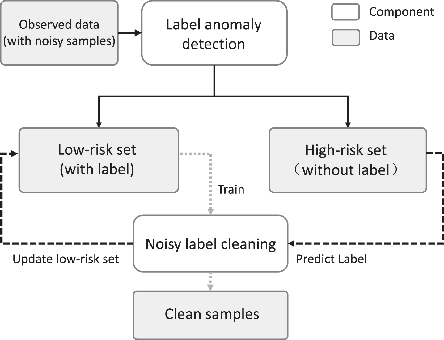
The LDAAD framework.

In the following, we elaborate on the two key components. Section 3.1 presents the label anomaly detection and the noisy label cleaning is detailed in Section 3.2.

3.1 Label anomaly detection

Based on the assumption that the samples belonging to the same class have similarities in their feature representations [32], we identify samples that are likely to be incorrectly labeled with an anomaly detection algorithm. The details of the label anomaly detection are shown in Algorithm 1. The original training set D is split into C subsets, denoted as D_i, following the given label (line 2). The label of all samples in each subset D_i is thus the same. We then apply an unsupervised anomaly detection algorithm on each subset D_i (lines 3-4) and add the samples which are judged as normal to the low-risk set G. The samples judged as abnormal are instead added to the high-risk set R (line 5).

Algorithm 1 Label anomaly detection

Input:

(1) Dataset with noisy labels D;

(2) Anomaly detection algorithm AD.

Output: low-risk dataset G, high-risk dataset R.

1: G =∅, R =∅

2: Split D by label into {D₁, D₂, . . . , D_C}

3: fori = 1 to Cdo

4: G_i, R_i = AD(D_i)

5: G = G ∪ G_i, R = R ∪ R_i

6: returnG, R

3.2 Noisy label cleaning

Algorithm 2 Label cleaning algorithm

Input:

(1) low-risk dataset (x, y) ∈ G, high-risk dataset x ∈ R;

(2) Number of folds K; (3) Iteration times M;

(4) Classifier clf.

Output: Clean dataset C.

1: G′ = {0}, R′ = {}, C =∅

2: form = 1 to Mdo

3: Split G into {G₁, G₂, . . . , G_K}

4: fork = 1 to Kdo

5: G^* = G \ G_k

6: f_k = clf.fit(G^*)

7: for (x_i, y_i) ∈ G_kdo

8: Predict

y_{i}^{'}

with f_k (x_i)

9: if (

y_{i}^{'} = = y_{i}

) then

10: G′ (x_i) = G′ (x_i) +1

11: forx_i ∈ Rdo

12: Predict

y_{i}^{'}

with f_k (x_i)

13: Append

y_{i}^{'}

to R′ (x_i)

14:forx_i ∈ Rdo

15:

c_{r} = \underset{y_{i}^{'}}{\arg max} {y^{'} | y^{'} \leftarrow R^{'} (x_{i})} / (K * M)

16: ifc_r > th_rthen

17:

y_{i}^{'} = {arg}_{y^{'}} {y^{'} | R^{'} (x_{i})}

18:

C = C \cup (x_{i}, y_{i}^{'})

19:for (x_i, y_i) ∈ Gdo

20: c_g = G′ (x_i)/(K * M)

21: ifc_g > th_gthen

22: C = C ∪ (x_i, y_i)

23:returnC

The samples in the low-risk set are filtered to remove any with low label confidence. For samples in the high-risk set, we predict a new label and retain any samples where we are highly confident in this new label being correct. The full details of the label cleaning procedure are delineated in Algorithm 2. The number of noisy samples in the low-risk set is believed to be less than the number of noise samples in the high-risk set, hence, the low-risk samples are used for model training. This assumption directly follows from the use of the anomaly detection algorithm in the sample partitioning.

In Algorithm 2, we follow the K-fold cross-validation scheme and randomly divide the low-risk set G into K subsets (line 3). For each subset G_k ∈ {G₁, G₂, . . . , G_K}, we train an anomaly classification model f_k on the remaining (K - 1) subsets G^* (lines 4-6). The labels of samples in G_k and R are predicted with f_k. For each sample (x_i, y_i) ∈ G, we keep count of the number of times the predicted label $y_{i}^{'}$ matches the given label y_i. For samples x_i ∈ R, we instead keep track of all the predicted values $y_{i}^{'}$ (lines 7 to 13). This K-fold cross-validation is run M times to reduce the variance in the predictions (line 2). Subsequently, each sample in the low-risk set G has a count of the number of times the predicted label matches the given label recorded in G′. The samples in R instead have an associated list in R′ with (K × M) predicted labels. For each sample x_i ∈ R, we identify the most common predicted label $y_{i}^{'}$ and its prediction ratio c_r as follows

$\begin{matrix} y_{i}^{'} & = \underset{y_{i}^{'}}{\arg max} {y_{i}^{'} | y_{i}^{'} \leftarrow R^{'} (x_{i})}, \\ c_{r} & = \frac{{max}_{y_{i}^{'}} {y_{i}^{'} | y_{i}^{'} \leftarrow R^{'} (x_{i})}}{K \times M}, \end{matrix}$ where $y_{i}^{'}$ denotes the predicted label of x_i and R′ (x_i) is the list of predicted labels for x_i. If the prediction ratio c_r is greater than a threshold th_r, the label is accepted and the sample $(x_{i}, y_{i}^{'})$ is added to the clean set C (lines 14-18).

Moreover, we only retain the samples most likely to be clean in the low-risk set G. Since these samples already have a reasonable given label, we consider how many times the given label matches the predicted label and generate a score as follows

$c_{g} = \frac{# of predictions where y^{'} equal to y}{K \times M} .$ For each sample (x_i, y_i), if and only if its corresponding c_g value is greater than a threshold th_g, we add it to the clean set C (lines 19-22).

It is worth noting that we retain the observed labels of the low-risk dataset G and filter them to remove samples with low confidence. The observed labels of the high-risk dataset R are discarded and the samples are instead relabeled. Therefore, part of the samples in C will retain the given label, while another part of the samples has been relabeled.

4 Evaluation

In this section, we evaluate LDAAD’s robustness and effectiveness. We begin by introducing the datasets and the evaluation metrics. We then present the baselines and their parameter settings. We subsequently present a performance comparison with the state-of-the-art baselines. Finally, we demonstrate the efficiency gains obtained by the various components of LDAAD through an ablation study and a parameter sensitivity analysis of the main model parameters.

4.1 Datasets and evaluation metrics

We use three real-world datasets collected from different fields. A summary of the datasets is given in Table 1.

Table 1
Dataset summary

Datasets |D_train| |D_test| # classes N # features

Mw 18, 477 6, 159 2 274

Thermostat 14, 958 5, 050 11 115

Tasks_q 112, 500 37, 000 4 26

Datasets	\|D_train\|	\|D_test\|	# classes N	# features
Mw	18, 477	6, 159	2	274
Thermostat	14, 958	5, 050	11	115
Tasks_q	112, 500	37, 000	4	26

Microwave (Mw) [20]: This dataset consists of 21 KPIs (Key Performance Indicators) from microwave base stations in a cellular network. The KPIs contain information about the performance status and health of the microwave links in the network. The data has a granularity of 15 minutes, and all data from 24 hours have been merged into a single record. Each record thus has a total of 2016 (96 × 21) values from which 274 features have been constructed. Each sample has been marked as normal or abnormal by domain experts, and the abnormal rate is about 7%.

Thermostat [33]: The dataset contains raw network traffic data under influence of different types of network attacks. A set of 23 features has been captured, including various statistics related to package size, count, and jitter. By using different aggregation variables and five different-sized time windows, 115 features are constructed. Each sample is marked as a normal operation (50%), or one of ten malicious attack types (5% each).

Tasks_q [34]: This is a dataset collected from an operational data center over 29 days. Each sample in the dataset corresponds to a cluster task and has 26 features, including task start and end time, host machine, resource utilization, etc. We focus on four event classes related to the termination of a task: EVICT, FAIL, FINISH, and KILL, which corresponds to normal (FINISH) and abnormal (EVICT, FAIL and KILL) termination states of a task. The distribution of these four classes are: FINISH 77.8%, FAIL 0.19%, EVICT 0.02%, and KILL 22%.

In order to avoid over-fitting, we select the top 75% samples of the Mw dataset sorted by time as training samples, and the remaining 25% as test samples. For the Thermostat and Tasks_q datasets, there is no time information, hence we randomly select 75% of samples for each dataset as the training set, and use the remaining 25% for evaluation.

To emulate label noise, we manually corrupt the labels in the training data while keeping the test set clean. For this purpose, we introduce a noise transition matrix T ∈ R^C×C where C is the number of classes and T_jk = P (y = k|y′ = j) characterize the probability of samples of the j-th class being flipped to the k-th class. For label corruption, we use two different noise injection methods, symmetric and asymmetric noise, defined as follows.

Definition 1 (symmetric noise) Given noise ratio ε, we define the noise transition matrix as T_jj = 1 - ε, j ∈ [C], and $T_{jk} = \frac{ε}{C - 1}, k \neq j, k \in [C]$ .

Definition 2 (asymmetric noise) Given noise ratio ε, T_jj = 1 - ε, j ∈ [C], and T_jk = ε, for some k ≠ j, k ∈ [C], otherwise T_jk = 0.

For symmetric noise, given a noise ratio ε, we uniformly flip the class label to one of the other classes. This assumes that the noise is independent of the true class label. Asymmetric noise, on the other hand, is class-dependent and constructed to imitate real-world noise. We flip a fraction ε of the labels to a similar class where the labels are often confused (e.g., 1 ↔ 7, truck → car).

We inject noise with different proportions ε into the three datasets and compare their performance. For evaluation, we use both accuracy and PRAUC (Precision-Recall Area Under Curve) as metrics. For highly imbalanced datasets, accuracy alone is not enough to judge the effectiveness of the model. This is especially the case in the binary classification tasks, we thus use PRAUC for performance evaluation on the binary classification dataset Mw, while accuracy is used for the multi-classification tasks datasets Thermostat and Tasks_q.

After using one of the de-noising methods to obtain a set of selected samples, the samples are used as training data to train a classifier. Subsequently, we use the trained classifier to predict the labels of the test samples and compute the evaluation metrics. Note that the labels in the test set are clean and no label noise has been injected.

4.2 Baselines and parameter settings

We select three representative algorithms for handling label noise as baselines in our performance evaluation, RAD [31], Co-teaching+ [28], and DivideMix [29]. Furthermore, we train a random forest-based classifier, denoted by RF, on the given samples without using any label de-noise algorithm as a control baseline. The parameters of each method are given below.

For LDAAD, we choose the unsupervised learning algorithm isolation forest [14] as the default anomaly detection algorithm (see Section 3.1). For the anomaly classification model (see Section 3.2), we apply two different classifiers, a random forest classifier (using 100 trees) and a GRU algorithm. The parameters are set as follows:

M: the number of iterations (default 5).

K: the number of cross-validation segments in each iteration (default 10).

th_g: high-risk sample screening threshold (default 0.7).

th_r: low-risk sample screening threshold (default 0.7).

For the baseline methods, RAD requires supplementary clean training data for initialization. We use 10, 100, and 1, 000 clean training samples in the experiments for this purpose. All other method-specific parameters use their default values. For DivideMix, we use a GRU as the classifier and keep other parameters unchanged. For the GRU itself (used by DivideMix and one of our LDAAD variants), we use a simple architecture with 2 hidden layers, each of size 10. Cross-entropy is used as the loss function. The Co-teaching+ baseline uses a 2-layer MLP with a hidden layer of size 256 using the ReLU activation function [35].

For the final training with the selected samples, LDAAD uses the same classifier as in the label cleaning step, either random forest [36] or GRU [37]. DivideMix, Co-teaching+, and RAD all use their original classifiers, i.e., GRU for DivideMix, MLP for Co-teaching+, and a random forest for RAD. Note that RAD uses an MLP in its original publication however in our experiments it consistently gives a worse result.

4.3 Comparison with the state-of-the-art

The accuracy of LDAAD and the baseline algorithms on the Thermostat and Tasks_q datasets are shown in Table 2. The baseline RF does not attempt to deal with label noise and is thus naturally the best when no noise is added (ε = 0) since its action of not removing or changing any labels is correct. We furthermore note that LDAAD is the second-best under this setting with a relatively small accuracy loss, indicating that LDAAD has a minimal detrimental effect when the label noise is low. In contrast, the other baselines have significant accuracy drops. For higher noise ratios, LDAAD achieves a significant improvement over the control RF baseline and, in most scenarios, outperforms the state-of-the-art algorithms. More specifically, LDAAD obtains a significantly higher accuracy on the Thermostat dataset compared to all baseline algorithms. On the Tasks_q dataset, both RAD_1000 and Co-teaching+ achieves accuracies comparable to LDAAD(GRU) for higher noise ratios (ε ∈ [0.4, 0.6]).

Table 2
Test accuracy on Thermostat and Tasks_q with symmetric noise. Algorithms marked with * have been re-implemented using open-source code

Dataset Thermostat Tasks_q Average

Method / Noise ratio 0.0 0.2 0.4 0.6 0.0 0.2 0.4 0.6

RF 95.0 93.3 89.3 81.1 92.8 83.7 67.5 44.8 80.9

RAD_10* 31.9 33.5 25.2 22.1 77.9 77.8 77.8 77.8 53.0

RAD_100* 80.2 73.9 66.7 58.1 79.1 78.4 77.0 77.8 73.9

RAD_1000* 88.1 86.7 78.4 77.6 80.8 80.8 80.7 79.2 80.1

Co-teaching+* 70.1 57.4 45.5 42.1 83.1 82.6 81.1 80.4 67.8

DivideMix* 88.6 88.2 85.5 83.2 84.5 78.6 76.9 76.9 82.8

LDAAD(RF) 95.0 94.9 94.7 93.7 91.4 86.6 78.5 59.2 86.8

LDAAD(GRU) 94.5 94.5 93.7 92.9 84.1 82.5 81.4 79.1 87.8

Dataset	Thermostat	Tasks_q	Average
RF	95.0	93.3	89.3	81.1	92.8	83.7	67.5	44.8	80.9
RAD_10*	31.9	33.5	25.2	22.1	77.9	77.8	77.8	77.8	53.0
RAD_100*	80.2	73.9	66.7	58.1	79.1	78.4	77.0	77.8	73.9
RAD_1000*	88.1	86.7	78.4	77.6	80.8	80.8	80.7	79.2	80.1
Co-teaching+*	70.1	57.4	45.5	42.1	83.1	82.6	81.1	80.4	67.8
DivideMix*	88.6	88.2	85.5	83.2	84.5	78.6	76.9	76.9	82.8
LDAAD(RF)	95.0	94.9	94.7	93.7	91.4	86.6	78.5	59.2	86.8
LDAAD(GRU)	94.5	94.5	93.7	92.9	84.1	82.5	81.4	79.1	87.8

For the two LDAAD variants, i.e., using RF or GRU as the classifier, the results are relatively equal on the Thermostat dataset, with RF having a slight edge. On the Tasks_q dataset, the GRU-based abnormal classification model obtains higher accuracy when the noise ratio is high, while the opposite is true for the scenario without label noise. When considering the average of all datasets and noise levels, LDAAD(GRU) outperforms LDAAD(RF) with 1% on the symmetric noise experiments. Furthermore, LDAAD(GRU) has a 5% relative improvement over DivideMix, the best baseline model.

The results on the Mw dataset are shown in Figure 2. In the absence of noise, RF and LDAAD(RF) achieves the best classification results, both with a PRAUC of 96%, outperforming the other baselines with a large margin. When label noise is present, RAD_1000 obtains the most consistent results overall, and in addition, it achieves the highest PRAUC scores when the noise ratio is high. For the algorithms that do not use clean sample initialization, LDAAD(GRU) obtains the best overall PRAUC scores. However, when the noise ratio reaches 60%, none of these algorithms perform well. These results imply that for the Mw dataset, the clean label initialization used by RAD has a significant impact and can help the algorithm better differentiate noisy samples. However, for noise ratios of 60%, our assumption that a majority of the samples are correctly labeled has been broken. Label noise ratios this high are very unusual in practice, especially for anomaly detection due to the inherent class imbalance.

Fig. 2

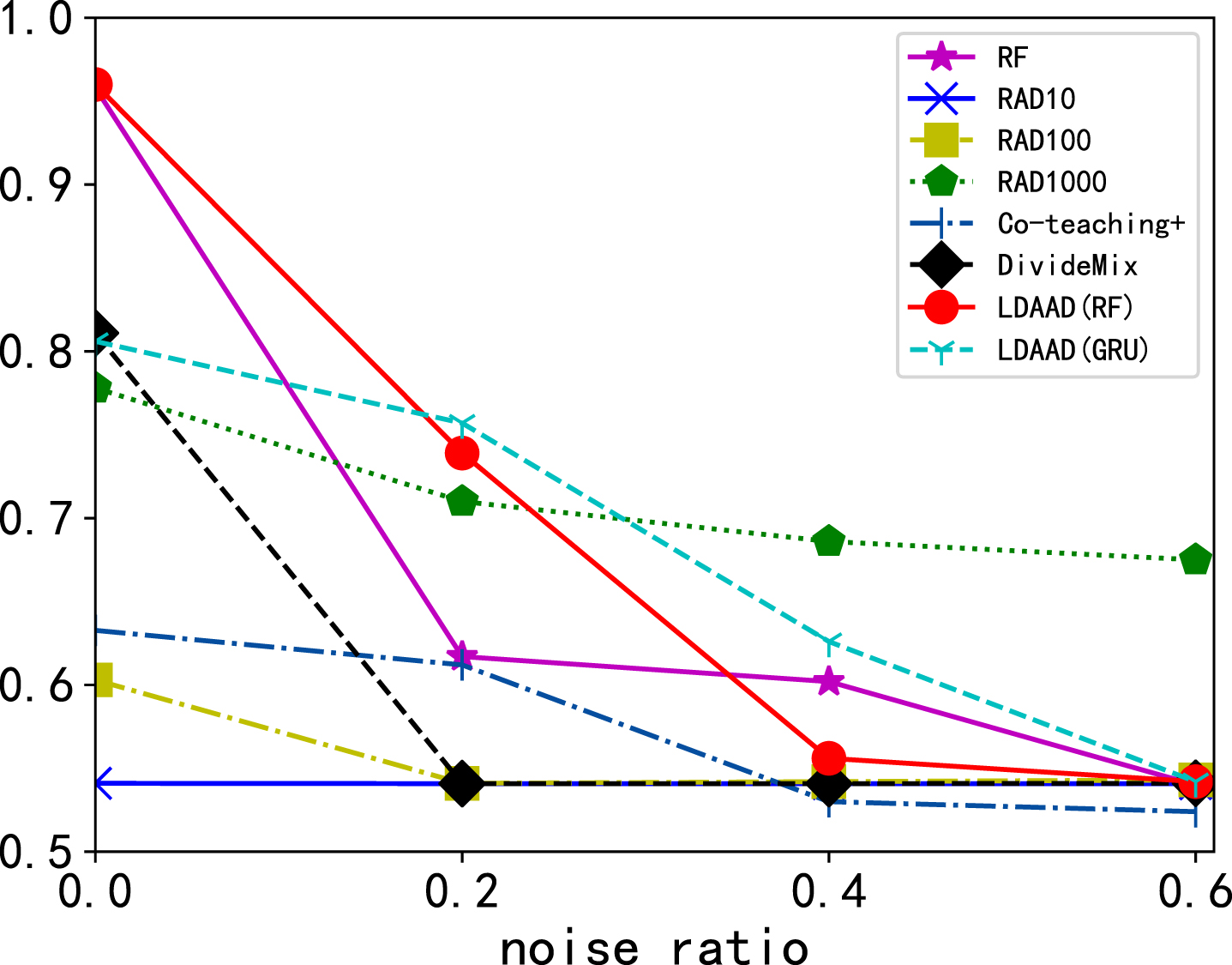
PRAUC results on Mw under symmetric noise.

We further corrupt the labels in the Thermostat training data with different levels of asymmetric noise. We randomly select several classes to modify and the labels are changed as follows: 9 → 1, 10 → 0, 3 ↔ 5, 4 → 7. The results are shown in Table 3. Overall, LDAAD(RF) achieves the best performance with noise ratios 0.2 and 0.4 while for 0.6, RAD_1000 obtains a better result. Similar to the observation on the Mw dataset, we believe that since the noise ratio is exceptionally high, the additional clean data initialization in RAD has a greater effect. When considering all three noise ratio settings together, LDAAD(RF) still outperforms RAD_1000 slightly, with a relative improvement of 2%. We also note that both versions of LDAAD significantly outperform Co-teaching+ and DivideMix when injecting asymmetric noise.

Table 3

Test accuracy on thermostat with asymmetric noise

Dataset	Thermostat
Method / Noise ratio	0.2	0.4	0.6
RF	94.0	89.5	77.8
RAD_10*	32.9	22.6	28.9
RAD_100*	70.5	69.3	59.8
RAD_1000*	88.7	87.9	86.7
Co-teaching+*	60.6	49.4	45.2
DivideMix*	85.4	81.2	73.8
LDAAD(RF)	94.6	92.7	81.1
LDAAD(GRU)	93.9	89.6	77.1

4.4 Ablation study

We perform an ablation study to demonstrate the effectiveness of the two main components in our proposed framework: the label anomaly detection (LAD) component and the noisy label cleaning (NLC) component.

First, we demonstrate the effectiveness of our proposed label anomaly detection component in performing the initial sample partitioning. To this end, we examine the noise ratio in the low-risk set after applying the LAD component. We utilize two typical unsupervised anomaly detection algorithms, isolation forest (iForest) and local outlier factor (LOF) [38]. The experiment is conducted on all three datasets with injected symmetric label noise with ratios 20%, 40%, and 60%. The result is illustrated in Figure 3.

Fig. 3

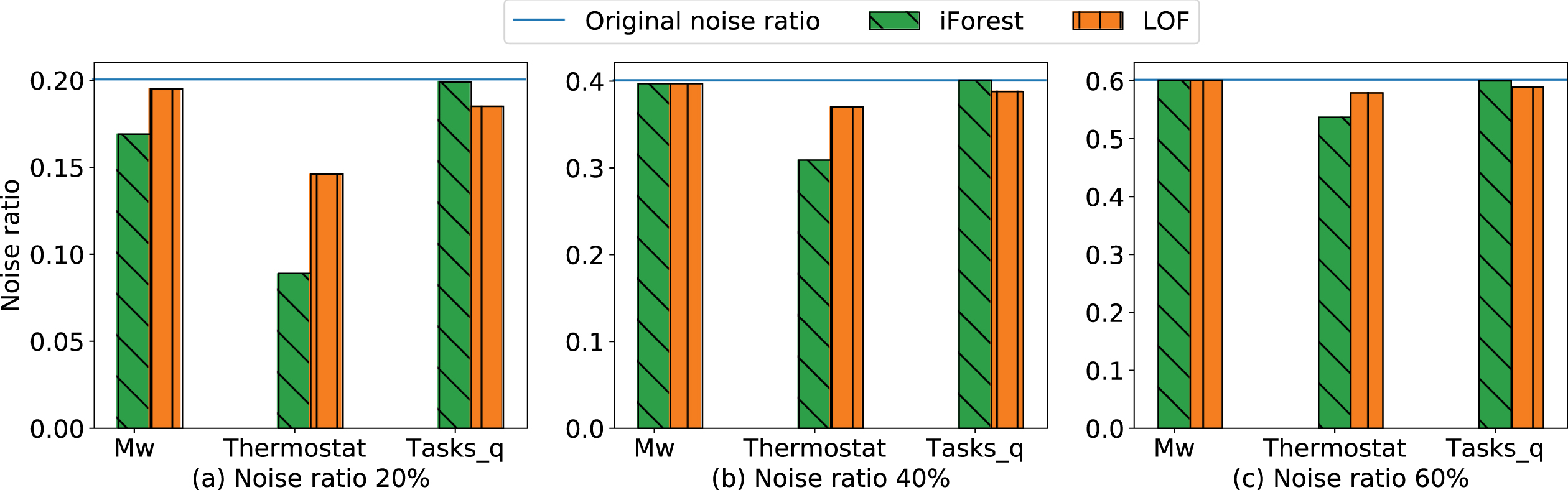
The label noise ratio in the low-risk sample set after applying the label anomaly detection component (lower is better). The original noise ratio is indicated by the vertical line in each subfigure.

We first make the wrap-up observation that the iForest algorithm achieves better overall results than the LOF algorithm. LOF works better on the Tasks_q dataset, but the difference is minimal. Furthermore, iForest has significantly better performance on Thermostat and for low noise ratios on Mw. Both algorithms have a negligible impact on Mw with noise ratios 0.4 and 0.6.

The LAD component has the most significant impact on the Thermostat dataset. Using the iForest algorithm, we observe a relative decrease in label noise of over 50% for ε = 0.2 to close to 12% for ε = 0.6. On the other two datasets, Mw and Tasks_q, we note that when the noise ratio is low (i.e., 20%), the LAD component reduces the label noise by around 2∼ 3 % in absolute terms. For higher label noise levels on these two datasets, the effect decreases and is not very significant. The dataset characteristics are a possible explanation for the observed behavior. These two datasets are highly unbalanced, and with an increase in artificial label noise, the number of incorrectly labeled samples in the minor classes may exceed the number of correctly labeled samples. This can confuse the anomaly detection algorithms. Nevertheless, the LAD component does not have a higher level of label noise in the low-risk set in any evaluated scenario, i.e., the LAD component does not worsen the situation. In summary, the LAD component can considerably reduce the noisy samples in the training set while not having any adverse effects in the worst case.

Furthermore, to provide more insights into how the two components contribute to the success of LDAAD, we show the effect of removing them one-by-one. Specifically, we examine two variations of LDAAD as follows:

LAD (RF): LDAAD with the NLC component removed. The final model is instead trained directly using G obtained from Algorithm 1.

NLC (RF): LDAAD with the LAD component removed. Each sample is randomly assigned to either R or G.

The results are shown in Table 4. First, we note that removing any component will generally cause performance degradation, highlighting the importance of each component. Specifically, the accuracy with only the LAD component is consistently lower than LDAAD, with an increasing disparity for higher noise ratios and when applying the more challenging asymmetric noise. On the other hand, running with only NLC has a lower performance impact, indicating that the NLC component is more important for the final result on the tested datasets.

Table 4

Ablation study in terms of test accuracy on Thermostat and Tasks_q

Dataset	Thermostat						Tasks_q
Noise type	Sym.				Asym.		Sym.
Method / Noise ratio	0.0	0.2	0.4	0.6	0.2	0.4	0.0	0.2	0.4	0.6
RF	95.0	93.3	89.3	81.1	94.0	89.5	92.8	83.7	67.5	44.8
LDAAD(RF)	95.0	94.9	94.7	93.7	94.6	92.7	91.4	86.6	78.5	59.2
LAD (RF)	94.1	94.4	93.8	90.6	92.7	88.5	89.1	86.2	78.3	58.9
NLC (RF)	94.8	94.5	94.1	92.9	93.8	91.9	91.2	83.7	78.7	59.9

As can be observed in Figure 3, the effectiveness of LAD on the Tasks_q dataset is minimal when using the iForest algorithm for ε ∈ [0.2, 0.4, 0.6]. This is reflected in the accuracy on Tasks_q, where the difference with and without LAD is minimal and, in some cases, applying LAD is slightly detrimental. On the other hand, removing LAD has a more significant performance impact on the Thermostat dataset.

A considerable performance drop is observed for higher noise ratios when both components are removed simultaneously (equivalent to the RF baseline). Furthermore, when no label noise is present, LDAAD has a minimal adverse effect while both variations, LAD (RF) and NLC (RF), both have larger negative impacts. The cooperation of the two components will thus mitigate any adverse side effects when the data have insignificant levels of label noise.

4.5 Parameter sensitivity analysis

We demonstrate how sensitive the result of LDAAD is to the various parameter settings. For this purpose, all parameters are set to their default values and kept constant while a single parameter is adjusted. We use LDAAD(GRU) and train on the Thermostat dataset with 40% symmetric noise. Figure 4 shows the results of the sensitivity analysis for each parameter. From the figures, we can observe that higher values for K and M will increase the performance, i.e., we obtain a cleaner dataset when these parameters are higher. However, higher M and K values also increase the algorithm running time, hence, this is a trade-off between speed and accuracy.

Fig. 4

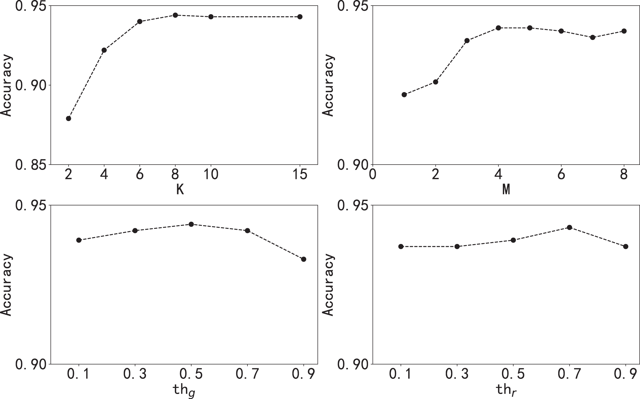
Parameter sensitivity analysis on Thermostat with 40% symmetric noise.

Moreover, we can observe that the best accuracy is obtained when the two threshold parameters th_g and th_r are between 0.5 and 0.7. A higher threshold will result in a relatively cleaner set of samples which is often preferred. We thus select 0.7 as the default value for both parameters.

5 Conclusion

In this paper, we propose an algorithm framework LDAAD that fuses unsupervised and semi-supervised learning to solve the problem of incorrectly labeled data samples in the area of anomaly detection. The algorithm screens out the incorrectly labeled samples and either corrects or discards them. To this end, we first group the samples according to the given label class, and any abnormal samples are detected separately within each group. Based on the anomaly detection results, we divide the dataset into two sets, low-risk and high-risk. The low-risk samples are used as training data for an ensemble of classifiers which we subsequently apply to predict the labels of all samples. We then retain any low-risk samples where the predicted label is frequently equal to the given label while discarding the rest. The samples in the high-risk set are either re-labeled with the most confident label or removed. We evaluate the effectiveness of our approach on three separate anomaly detection datasets and demonstrate that LDAAD performs better or in line with all baselines for different noise types and noise magnitudes.

References

, Li

, Wang

and Wang

, A deep learning approach foranomaly detection based on SAE and LSTM in mechanical equipment, The International Journal of Advanced Manufacturing Technology 103(1–4) (2019), 499–510.

Pan

, Zhang

, Lee

P.P.

, Cheng

, He

and Zhang

, An intelligent customer care assistant system for large-scale cellular network diagnosis, in: Proceedings of the 23rd ACM International Conference on Knowledge Discovery and Data Mining, (2017), pp. 1951–1959.

Garg

, Kaur

, Kumar

, Kaddoum

, Zomaya

A.Y.

and Ranjan

, Ahybrid deep learning-based model for anomaly detection in clouddatacenter networks, IEEE Transactions on Network and ServiceManagement 16(3) (2019), 924–935.

, Mendis

G.J.

and Wei

, Real-time detection of false datainjection attacks in smart grid: A deep learning-based intelligentmechanism, IEEE Transactions on Smart Grid 8(5) (2017), 2505–2516.

West

and Bhattacharya

, Intelligent financial fraud detection:a comprehensive review, Computers & Security 57 (2016), 47–66.

Frénay

and Verleysen

, Classification in the presence oflabel noise: a survey, IEEE Transactions on Neural Networks and Learning Systems 25(5) (2013), 845–869.

Zhang

, Bengio

, Hardt

, Recht

and Vinyals

, Understanding deep learning requires rethinking generalization, ICLR (2017).

Xiao

, Xia

, Yang

, Huang

and Wang

, Learning from massive noisy labeled data for image classification, in: Proceedings of the 28th IEEE Conference on Computer Vision and pattern recognition, (2015), pp. 2691–2699.

Vahdat

, Toward robustness against label noise in training deep discriminative neural networks, in: Proceedings of the 31st International Conference on Neural Information Processing Systems, (2017), pp. 5596–5605.

10.

, Yang

, Song

, Cao

, Luo

and Li

L.-J.

, Learning from noisy labels with distillation, in: Proceedings of the 16th IEEE Conference on Computer Vision and Pattern Recognition, (2017), pp. 1910–1918.

11.

Patrini

, Rozza

and Krishna

, Making deep neural networks robust to label noise: A loss correction approach, in: Proceedings of the 16th IEEE Conference on Computer Vision and Pattern Recognition, (2017), pp. 1944–1952.

12.

Ghosh

, Kumar

and Sastry

, Robust loss functions under label noise for deep neural networks, in: Proceedings of the AAAI Conference on Artificial Intelligence, Vol. 31, 2017.

13.

Chalapathy

and Chawla

, Deep learning for anomaly detection: A survey, arXiv preprint arXiv:1901.03407 (2019).

14.

Liu

F.T.

, Ting

K.M.

and Zhou

Z.-H.

,Isolation forest, in: Proceedings of the 8th IEEE International Conference on Data Mining, (2008), pp. 413–422.

15.

Ruff

, Zemlyanskiy

, Vandermeulen

, Schnake

and Kloft

, Self-Attentive, Multi-Context One-Class Classification for Unsupervised Anomaly Detection on Text, in: Proceedings of the 57th Annual Meeting of the Association for Computational Linguistics, (2019), pp. 4061–4071.

16.

Akcay

, Atapour-Abarghouei

and Breckon

T.P.

, Ganomaly: Semi-supervised anomaly detection via adversarial training, in: Proceedings of the 14th Asian Conference on Computer Vision, (2018), pp. 622–637.

17.

Blanchard

, Lee

and Scott

, Semi-supervised noveltydetection, The Journal of Machine Learning Research 11(2010), 2973–3009.

18.

Oliver

, Odena

, Raffel

C.A.

, Cubuk

E.D.

and Goodfellow

, Realistic evaluation of deep semi-supervised learning algorithms, in: Proceedings of the 32nd Conference on Neural Information Processing Systems, (2018), pp. 3235–3246.

19.

, Lee

P.P.

, Li

, Pan

and Zhang

, Cellpad: Detecting performance anomalies in cellular networks via regression analysis, in: Proceedings of the 17th IFIP Networking Conference, (2018), pp. 1–9.

20.

Pan

, Zhang

, Lee

P.P.

, Kalander

, Ye

and Wang

, Proactive microwave link anomaly detection in cellular datanetworks, Computer Networks 167 (2020), 106969.

21.

Hasan

, Islam

M.M.

, Zarif

M.I.I.

and Hashem

, Attack and anomalydetection in IoT sensors in IoT sites using machine learningapproaches, Internet of Things 7 (2019), 100059.

22.

Hendrycks

, Mazeika

, Wilson

and Gimpel

, Using trusted data to train deep networks on labels corrupted by severe noise, in: Proceedings of the 32nd Conference on Neural Information Processing Systems, (2018), pp. 10456–10465.

23.

Ghosh

, Manwani

and Sastry

, Making risk minimizationtolerant to label noise, Neurocomputing 160 (2015), 93–107.

24.

Wang

, Ma

, Chen

, Luo

, Yi

and Bailey

, Symmetric cross entropy for robust learning with noisy labels, in: Proceedings of the IEEE International Conference on Computer Vision, (2019), pp. 322–330.

25.

Zhang

and Sabuncu

, Generalized cross entropy loss for training deep neural networks with noisy labels, in: Proceedings of the 32nd Conference on Neural Information Processing Systems, (2018), pp. 8778–8788.

26.

Jiang

, Zhou

, Leung

, Li

L.-J.

and Fei-Fei

, Mentornet: Learning data-driven curriculum for very deep neural networks on corrupted labels, in: Proceedings of the 35th International Conference on Machine Learning, (2018), pp. 2304–2313.

27.

Han

, Yao

, Yu

, Niu

, Xu

, Hu

and Tsang

, Co-teaching: Robust training of deep neural networks with extremely noisy labels, in: Proceedings of the 32nd Conference on Neural Information Processing Systems, (2018), pp. 8527–8537.

28.

, Han

, Yao

, Niu

, Tsang

, Sugiyama

, How does disagreement help generalization against label corruption?, in: Proceedings of the 36th International Conference on Machine Learning, 2019.

29.

, Socher

and Hoi

S.C.

, DivideMix: Learning with Noisy Labels as Semi-supervised Learning, in: Proceedings of the 8th International Conference on Learning Representations, 2019.

30.

Zhong

J.-X.

, Li

, Kong

, Liu

, Li

T.H.

and Li

, Graph convolutional label noise cleaner: Train a plug-and-play action classifier for anomaly detection, in: Proceedings of the IEEE Conference on Computer Vision and Pattern Recognition, (2019), pp. 1237–1246.

31.

Zhao

, Cerf

, Birke

, Robu

, Bouchenak

, Mokhtar

S.B.

and Chen

L.Y.

, Robust anomaly detection on unreliable data, in: Proceedings of the 49th Annual IEEE/IFIP International Conference on Dependable Systems and Network, (2019), pp. 630–637.

32.

Chen

, Garcia

E.K.

, Gupta

M.R.

, Rahimi

and Cazzanti

, Similarity-based classification: Concepts and algorithms, Journal of Machine Learning Research 10(3) (2009).

33.

Meidan

, Bohadana

, Mathov

, Mirsky

, Shabtai

, Breitenbacher

and Elovici

, N-baiot—network-based detectionof iot botnet attacks using deep autoencoders, IEEE PervasiveComputing 17(3) (2018), 12–22.

34.

Reiss

, Wilkes

and Hellerstein

J.L.

, Google cluster-usage traces: format+ schema, Google Inc., White Paper (2011), 1–14.

35.

Agarap

A.F.

, Deep learning using rectified linear units (relu), arXiv preprint arXiv:1803.08375 (2018).

36.

Breiman

, Random forests, Machine Learning 45(1) (2001), 5–32.

37.

Cho

, Van Merriënboer

, Gulcehre

, Bahdanau

, Bougares

, Schwenk

and Bengio

, Learning phrase representations using RNN encoder-decoder for statistical machine translation, arXiv preprint arXiv:1406.1078 (2014).

38.

Breunig

M.M.

, Kriegel

H.-P.

, Ng

R.T.

and Sander

, LOF: identifying density-based local outliers, in: Proceedings of the 2000 ACM SIGMOD international conference on Management of data, (2000), pp. 93–104.

LDAAD: An effective label de-noising approach for anomaly detection

Abstract

Keywords

1 Introduction

2 Related Work

2.1 Machine learning-based anomaly detection

2.2 Learning with noisy labels

3 LDAAD Design

3.2 Noisy label cleaning

4 Evaluation

4.1 Datasets and evaluation metrics

Table 1 Dataset summary Datasets |D train | |D test | # classes N # features Mw 18, 477 6, 159 2 274 Thermostat 14, 958 5, 050 11 115 Tasks_q 112, 500 37, 000 4 26

4.3 Comparison with the state-of-the-art

References

Table 1
Dataset summary

Datasets |D_train| |D_test| # classes N # features

Mw 18, 477 6, 159 2 274

Thermostat 14, 958 5, 050 11 115

Tasks_q 112, 500 37, 000 4 26