Uncertain support vector regression with imprecise observations

Abstract

Traditional support vector regression dedicates to obtaining a regression function through a tube, which contains as many as precise observations. However, the data sometimes cannot be imprecisely observed, which implies that traditional support vector regression is not applicable. Motivated by this, in this paper, we employ uncertain variables to describe imprecise observations and build an optimization model, i.e., the uncertain support vector regression model. We further derive the crisp equivalent form of the model when inverse uncertainty distributions are known. Finally, we illustrate the application of the model by numerical examples.

Keywords

Imprecise observations uncertain variables support vector regression uncertainty theory

1 Introduction

Support vector regression was first introduced by Vapnik [23] to explore the relationship between explanatory variables and response variables through a tube, which is uniquely determined by a function and the radius of the tube. Different from other regression methods, support vector regression selects a regression function by minimizing some errors of the observations. Up to now, support vector regression has achieved excellent performances [2 , 19] in real-world applications, such as exchange rate forecasting [8, 21] and stock price forecasting [6]. More details about support vector regression can be found in overviews [20 , 25].

The tacit assumption in traditional support vector regression is that the observations are always crisp. However, the data are difficult or impossible to be precisely observed in some cases. It implies that the traditional support vector regression cannot be applied to such a problem. As an alternative method of solving the problem with imprecise observations, Liu [11, 13] introduced uncertain variables to describe imprecise data. The regression problems with imprecisely observed data [28] were discussed based on the assumption. Then, some studies about imprecise observations emerge in different fields. For time series analysis with imprecise observations, the idea has been explored, and several models have been proposed [26, 27]. The problem of testing the estimating results [15 , 29] and forecasting [9] were also investigated. For classification problems, the distance from an uncertain vector to a hyperplane was defined [7], and a hard margin uncertain support vector machine was given for separating linearly α-separable data sets.

Among the researches, regression problems with imprecise observations is an important topic. In fact, there have been extensive researches. The first attempt was given by Yao and Liu [28], who proposed least squares method for regression problems. Then on the one hand, different methods, such as least absolute deviations [17], lasso method [18] and ridge method [1] have been proposed to improve the robustness of the least squares method. On the other hand, different regression models were explored in the framework of uncertainty theory. For example, Fang and Hong [4] derived the crisp equivalent forms of different models under logarithmic, square root and reciprocal transformations. Song and Fu [22] derived the analytical expressions for the uncertain multivariable linear regression model by generalized least squares estimate. Hu and Gao [5] explored the properties of Gompertz regression model. However, the above methods focus on all losses from each observation. While the support vector regression function is determined by observations with heavy losses.

This paper dedicates to extending a support vector regression model to explore the relationship between the response variable and explanatory variables reviewed by the imprecise data. First, we employ uncertain variables to model imprecise data. Then we build an uncertain support vector regression model based on the maximum distance from observations to a hyperplane. It is distinct from random support vector models, which assume that the distribution is sufficiently close to its true frequency. In addition to giving a model, we also conduct numerical examples to illustrate the application of the proposed model.

The outline of the remaining paper is as follows. Section 2 lists some necessary definitions and theorems in uncertainty theory. Then Section 3 introduces the uncertain support vector regression model. Section 4 presents examples to illustrate the application of the model before concluding in Section 5.

2 Preliminaries

SectionPreliminaries This section reviews some necessary definitions and theorems used in the rest of the paper.

Let Ł be a σ-algebra on a nonempty set Γ . Liu [10, 11] defined that a set function M : Ł → [0, 1] is called an uncertain measure if it satisfies: (1) M {Γ} =1 for the universal set Γ; (2) M {Λ} + M {Λ^c} =1 for any Λ∈ Ł (3) For every countable sequence Λ₁, Λ₂, ⋯ ∈ Ł, $M {⋃_{i = 1}^{\infty} Λ_{i}} \leq \sum i = 1 \infty M {Λ_{i}};$ (4)The product uncertain measure M is an uncertain measure satisfying $M {\prod_{i = 1}^{\infty} Λ_{k}} = ⋀_{i = 1}^{\infty} M_{k} {Λ_{k}},$ where Λ_k are arbitrarily chosen events from Ł_k for k = 1, 2, …, respectively.

The triple (Γ_k, Ł _k, M_k) is called an uncertainty space. Then Liu [10] defined an uncertain variable τ as a measurable function from an uncertainty space (Γ, Ł , M) to the set of real numbers, i.e., the set {τ ∈ B} = {γ ∈ Γ ∣ τ (γ) ∈ B} belongs to Ł for any Borel set B. The function $ϒ (x) = M {τ \leq x}, x \in R$ is called the uncertainty distribution of τ.

Theorem 1. (Liu [12]) Let ξ₁, ξ₂, …, ξ_n be independent uncertain variables with inverse uncertainty distributions $Φ_{1}^{- 1}, Φ_{2}^{- 1}, \dots, Φ_{n}^{- 1}$ , respectively. If f is strictly increasing with respect to ξ₁, ξ₂, …, ξ_m and strictly decreasing with respect to ξ_m+1, ξ_m+2, …, ξ_n, then ξ = f (ξ₁, ξ₂, …, ξ_n) is an uncertain variable with inverse uncertainty distribution $\begin{matrix} Ψ^{- 1} (u) = f ( & Φ_{1}^{- 1} (u), \dots, Φ_{m}^{- 1} (u), \\ Φ_{m + 1}^{- 1} (1 - u), \dots, Φ_{n}^{- 1} (1 - u)) . \end{matrix}$

Theorem 2. (Liu [14]) Let ξ be an uncertain variable with inverse uncertainty distribution Φ^-1 (u). Then the expected value of |ξ| is $E [| ξ |] = \int_{0}^{1} Φ^{- 1} (u) intd u .$

Definition 1. (Qin and Li [18]) Let pmbξ = (ξ₁, ξ₂, …, ξ_n) be an n-dimensional uncertain vector. Suppose w^Tx + b = 0 is a hyperplane, where w = (w₁, w₂, …, w_n) is an n-dimensional vector with an Euclidean norm ∥w∥, x ∈ Rⁿ is an n-dimensional vector, and b is a scalar. Then the distance from pmbξ to the hyperplane H : w^Tx + b = 0 is defined as $d (ξ, H) = E [\frac{| w^{T} ξ + b |}{∥ w ∥}] .$

Theorem 3. (Liu [14]) Assume the constraint function g (x, ξ₁, ξ₂, …, ξ_n) is strictly increasing with respect to ξ₁, ξ₂, …, ξ_k and strictly decreasing with respect to ξ_k+1, ξ_k+2, …, ξ_n. If ξ₁, ξ₂, …, ξ_n are independent variables with inverse uncertainty distributions $Φ_{1}^{- 1}, Φ_{2}^{- 1}, \dots, Φ_{n}^{- 1},$ respectively, then the chance constraint $M {g (x, ξ_{1}, ξ_{2}, \dots, ξ_{n}) \leq 0} \geq α$ holds if and only if $\begin{matrix} g (x, Φ_{1}^{- 1} (α), \dots, Φ_{k}^{- 1} (α), \\ Φ_{k + 1}^{- 1} (1 - α), \dots, Φ_{n}^{- 1} (1 - α)) \leq 0 . \end{matrix}$

3 Uncertain support vector regression

Suppose that ${\tilde{x}}_{1}$ , ${\tilde{x}}_{2}, \dots$ , ${\tilde{x}}_{l}$ are the imprecise observations of explanatory vector $\tilde{x}$ , and ${\tilde{y}}_{1}$ , ${\tilde{y}}_{2}, \dots$ , ${\tilde{y}}_{l}$ are the imprecise observations of response variable $\tilde{y}$ . We want to model the relationship between $\tilde{y}$ and $\tilde{x}$ based on these imprecise observations.

As stated above, ${\tilde{x}}_{i} = ({\tilde{x}}_{i 1}, {\tilde{x}}_{i 2}, \dots, {\tilde{x}}_{in})$ is assumed to be an n dimensional uncertain vector, and ${\tilde{y}}_{i}$ is assumed to be an uncertain variable for i = 1, 2, …, l. Uncertain support vector regression aims to look for a function y = w^Tx + b to fit the observations $({\tilde{x}}_{1}, {\tilde{y}}_{1})$ , $({\tilde{x}}_{2}, {\tilde{y}}_{2})$ , …, $({\tilde{x}}_{l}, {\tilde{y}}_{l})$ . Here $w \in R^{n}$ is an n dimensional vector, and b is a real number. The function y = w^Tx + b exactly describes a hyperplane H : w^Tx - y + b = 0.

It follows from Definition 1 that the distance from uncertain vector $({\tilde{x}}_{i}^{T}, {\tilde{y}}_{i})$ to the hyperplane H is $\begin{matrix} d (({\tilde{x}}_{i}^{T}, {\tilde{y}}_{i}), H) = & E [\frac{(w^{T}, - 1) \cdot ({\tilde{x}}_{i}^{T}, {\tilde{y}}_{i})^{T} + b}{∥ (w^{T}, - 1) ∥}] \\ = & E [\frac{| w^{T} {\tilde{x}}_{i} - {\tilde{y}}_{i} + b |}{\sqrt{∥ w ∥^{2} + 1}}] . \end{matrix}$ Given pmbw and b, a smaller distance indicates that ${\tilde{y}}_{i}$ and its fitted value $w^{T} {\tilde{x}}_{i} + b$ are closer.

We choose $max_{1 \leq i \leq l} E [\frac{| w^{T} {\tilde{x}}_{i} - {\tilde{y}}_{i} + b |}{\sqrt{∥ w ∥^{2} + 1}}]$ as the distance from the set ${({\tilde{x}}_{1}, {\tilde{y}}_{1}), ({\tilde{x}}_{2}, {\tilde{y}}_{2}), \dots,$ $({\tilde{x}}_{l}, {\tilde{y}}_{l})}$ to the hyperplane H. The tube is thus determined by the hyperplane and the distance. The hyperplane and the tube are plotted in Fig. 1.

When the distance is minimized, each ${\tilde{y}}_{i}$ is close to its fitted value $w^{T} {\tilde{x}}_{i} + b$ as possible for i = 1, 2, …, l. Thus, we set $min_{w, b} max_{1 \leq i \leq l} E [\frac{| w^{T} {\tilde{x}}_{i} - {\tilde{y}}_{i} + b |}{\sqrt{∥ w ∥^{2} + 1}}]$ as the objective function.

Let ∈ > 0 be a real number. In this work, we assume that the function $w^{T} \tilde{x} + b$ has at most ∈ deviation from the actually obtained target ${\tilde{y}}_{i}$ for each ${\tilde{x}}_{i}$ in the sense of uncertain measure. In other words, we require the following constraints $M {w^{T} {\tilde{x}}_{i} + b - {\tilde{y}}_{i} \leq \in} \geq α_{i}, i = 1, 2, \dots, l$ (1) and $M {w^{T} {\tilde{x}}_{i} + b - {\tilde{y}}_{i} \geq - \in} \geq β_{i}, i = 1, 2, \dots, l,$ (2) where α_i and β_i are given confidence levels for i = 1, 2, …, l. We formulate the following uncertain support vector regression model ${\begin{matrix} min_{w, b} & max_{1 \leq i \leq l} E [\frac{| w^{T} {\tilde{x}}_{i} - {\tilde{y}}_{i} + b |}{\sqrt{∥ w ∥^{2} + 1}}] \\ s . t . & M {w^{T} {\tilde{x}}_{i} + b - {\tilde{y}}_{i} \leq \in} \geq α_{i}, \\ i = 1, 2, \dots, l, \\ M {w^{T} {\tilde{x}}_{i} + b - {\tilde{y}}_{i} \geq - \in} \geq β_{i}, \\ i = 1, 2, \dots, l . \end{matrix}$ (3)

Fig. 1

The tube determined by a hyperplane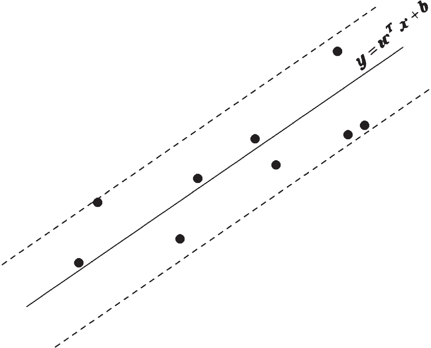

Next, we explore the crisp equivalent form of Model (3). When the inverse uncertainty distribution of the observations are known, we have the following result.

Theorem 4. Assume that the components of each uncertain vector ${\tilde{x}}_{i}$ are independent. Denote $Φ_{ij}^{- 1}$ and $Ψ_{i}^{- 1}$ as the inverse uncertainty distributions of ${\tilde{x}}_{ij}$ and ${\tilde{y}}_{i}$ , respectively. Then Model (3) has the following crisp equivalent form ${\begin{matrix} min_{w_{1}, \dots, w_{n}, b} & max_{1 \leq i \leq l} \int_{0}^{1} | \sum_{j = 1}^{n} w_{j} ϒ_{ij}^{- 1} (u, w_{j}) - Ψ_{i}^{- 1} (1 - u) + b | d u / \sqrt{\sum_{j = 1}^{n} w_{j}^{2} + 1} \\ s . t . & \sum_{j = 1}^{n} w_{j} ϒ_{ij}^{- 1} (α_{i}, w_{j}) - Ψ_{i}^{- 1} (1 - α_{i}) + b \leq \in, i = 1, 2, \dots, l \\ \sum_{j = 1}^{n} w_{j} ϒ_{ij}^{- 1} (β_{i}, - w_{j}) - Ψ_{i}^{- 1} (β_{i}) + b \geq - \in, i = 1, 2, \dots, l, \end{matrix}$ where $\begin{matrix} ϒ_{ij}^{- 1} (α_{i}^{*}, w_{j}^{*}) \\ = Φ_{ij}^{- 1} (α_{i}^{*}) \cdot I_{{w_{j}^{*} \geq 0}} + Φ_{ij}^{- 1} (1 - α_{i}^{*}) \cdot I_{{w_{j}^{*} < 0}}, \end{matrix}$ $α_{i}^{*}$ are arbitrarily chosen from {α_i, β_i, u}, respectively, and $w_{j}^{*}$ are arbitrarily chosen from {w_j, - w_j}, i = 1, 2, …, l, j = 1, 2, …, n, respectively.

Proof. The inverse uncertainty distribution of $w^{T} {\tilde{x}}_{i} + b - {\tilde{y}}_{i} - \in = \sum_{j = 1}^{n} w_{j} {\tilde{x}}_{ij} - {\tilde{y}}_{i} + b - \in$ is $F_{1 i}^{- 1} (u) = \sum_{j = 1}^{n} w_{j} ϒ_{ij}^{- 1} (u, w_{j}) - Ψ_{i}^{- 1} (1 - u) + b - \in .$ It follows from Theorem 3 that inequality (1) holds if and only if $\begin{matrix} F_{1 i}^{- 1} (α_{i}) & = \sum_{j = 1}^{n} w_{j} ϒ_{ij}^{- 1} (α_{i}, w_{j}) \\ - Ψ_{i}^{- 1} (1 - α_{i}) + b - \in \leq 0, \end{matrix}$ (5) which is the first constraint of Model (4). Similarly, the inverse uncertainty distribution of ${\tilde{y}}_{i} - w^{T} {\tilde{x}}_{i} - b - \in = {\tilde{y}}_{i} - \sum_{j = 1}^{n} w_{j} {\tilde{x}}_{ij} - b - \in$ is $F_{2 i}^{- 1} (u) = Ψ_{i}^{- 1} (u) - \sum_{j = 1}^{n} w_{j} ϒ_{ij}^{- 1} (u, - w_{j}) - b - \in .$ Similarly, inequality (2) holds if and only if $\begin{matrix} F_{2 i}^{- 1} (β_{i}) & = Ψ_{i}^{- 1} (β_{i}) - \sum_{j = 1}^{n} w_{j} ϒ_{ij}^{- 1} (β_{i}, - w_{j}) - b - \in \\ \leq 0, \end{matrix}$

which is the second constraint of Model (4). It follows immediately from Theorem 1 that the inverse uncertainty distribution of

$\frac{w^{T} {\tilde{x}}_{i} - {\tilde{y}}_{i} + b}{\sqrt{∥ w ∥^{2} + 1}}$ is $\frac{\sum_{j = 1}^{n} w_{j} ϒ_{ij}^{- 1} (u, w_{j}) - Ψ_{i}^{- 1} (1 - u) + b}{\sqrt{\sum_{j = 1}^{n} w_{j}^{2} + 1}} .$ According to Theorem 2, we obtain

$\begin{matrix} E [\frac{| w^{T} {\tilde{x}}_{i} - {\tilde{y}}_{i} + b |}{\sqrt{∥ w ∥^{2} + 1}}] = \frac{1}{\sqrt{\sum_{j = 1}^{n} w_{j}^{2} + 1}} \cdot \\ \int_{0}^{1} | \sum_{j = 1}^{n} w_{j} ϒ_{ij}^{- 1} (u, w_{j}) - Ψ_{i}^{- 1} (1 - u) + b | d u . \end{matrix}$

The theorem is completed.

4 Numerical experiments

In this section, we illustrate the application of uncertain support vector regression by numerical examples.

We suppose that all the imprecise observations are characterized by linear uncertain variables. The uncertainty distribution and the inverse uncertainty distribution of a linear uncertain variable Ł (a, b) is $Φ (x) = {\begin{matrix} 0, & if x \leq a \\ \frac{x - a}{b - a}, & if a < x \leq b \\ 1, & if b < x \end{matrix}$ and $Φ^{- 1} (u) = (1 - u) a + ub,$ respectively.

Example 1. We first consider a case of n = 1 and l = 15. That is to say, there is only one explanatory variable $\tilde{x}$ , and the data set is consisted of 15 imprecise observations. Let $Φ_{i}^{- 1}$ and $Ψ_{i}^{- 1}$ denote the inverse uncertainty distributions of ${\tilde{x}}_{i}$ and ${\tilde{y}}_{i}$ , respectively, for i = 1, 2, …, 15. The detailed data are shown in Table 1.

Table 1
Imprecise observations in Example 1

No. 1 2 3

${\tilde{x}}_{i}$ Ł(27, 28) Ł(16, 17) Ł(3, 4)

${\tilde{y}}_{i}$ Ł(62, 63) Ł(40, 41) Ł(13, 14)

No. 4 5 6

${\tilde{x}}_{i}$ Ł(25, 26) Ł(10, 11) Ł(9, 10)

${\tilde{y}}_{i}$ Ł(53, 54) Ł(23, 24) Ł(24, 25)

No. 7 8 9

${\tilde{x}}_{i}$ Ł(22, 23) Ł(0, 1) Ł(1, 2)

${\tilde{y}}_{i}$ Ł(51, 52) Ł(11, 12) Ł(12, 13)

No. 10 11 12

${\tilde{x}}_{i}$ Ł(20, 21) Ł(18, 19) Ł(16, 17)

${\tilde{y}}_{i}$ Ł(50, 51) Ł(40, 41) Ł(34, 35)

No. 13 14 15

${\tilde{x}}_{i}$ Ł(22, 23) Ł(7, 8) Ł(13, 14)

${\tilde{y}}_{i}$ Ł(46, 47) Ł(19, 20) Ł(32, 33)

No.	1	2	3
${\tilde{x}}_{i}$	Ł(27, 28)	Ł(16, 17)	Ł(3, 4)
${\tilde{y}}_{i}$	Ł(62, 63)	Ł(40, 41)	Ł(13, 14)
No.	4	5	6
${\tilde{x}}_{i}$	Ł(25, 26)	Ł(10, 11)	Ł(9, 10)
${\tilde{y}}_{i}$	Ł(53, 54)	Ł(23, 24)	Ł(24, 25)
No.	7	8	9
${\tilde{x}}_{i}$	Ł(22, 23)	Ł(0, 1)	Ł(1, 2)
${\tilde{y}}_{i}$	Ł(51, 52)	Ł(11, 12)	Ł(12, 13)
No.	10	11	12
${\tilde{x}}_{i}$	Ł(20, 21)	Ł(18, 19)	Ł(16, 17)
${\tilde{y}}_{i}$	Ł(50, 51)	Ł(40, 41)	Ł(34, 35)
No.	13	14	15
${\tilde{x}}_{i}$	Ł(22, 23)	Ł(7, 8)	Ł(13, 14)
${\tilde{y}}_{i}$	Ł(46, 47)	Ł(19, 20)	Ł(32, 33)

In order to obtain the optimal value (w, b) of function y = wx + b, we formulate Model (6) according to the uncertain support vector regression model.

We want to know how the optimal solutions to Model (6) change with different confidence levels and different accuracy parameters. Let parameters α_i = β_i ∈ {0.90, 0.95, 0.99} for i = 1, 2, …, 15, and let ∈ ∈{10, 9, 8, 7, 6} . Then we employ the function ‘fmincon’ in Matlab to solve Model (6) and the obtained results are presented in Table 2.

Table 2

Optimal solutions (w, b) to Model 6) under different ∈ and α

α	∈	w ₁	b
	10	1.9268	6.8544
	9	1.9239	6.9073
0.90	8	1.9499	6.4266
	7	1.9456	6.5073
	6	1.9500	6.4250
α	∈	w ₁	b
	10	1.9255	6.8786
	9	1.9225	6.9335
0.95	8	1.9181	7.0145
	7	1.9500	6.4250
	6	1.9500	6.4250
α	∈	w ₁	b
	10	1.9247	6.8928
	9	1.9213	6.9555
0.99	8	1.9167	7.0416
	7	1.9500	6.4250
	6	1.9500	6.4250

When the confidence level α = 0.95 and accuracy parameter ∈ = 6, the optimal function is y = 1.9500x + 6.4250. The function and the tube with radius 6 is plotted in Fig. 2.

Fig. 2

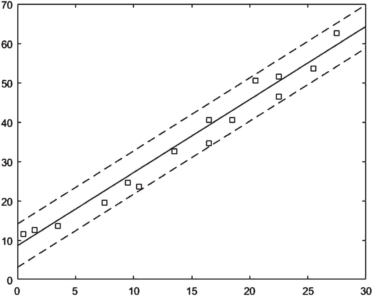
The result generated from Model (6) when α = 0.95, ∈ = 6.

The optimal function, y = 1.9500x + 6.4250, can be employed to predict a new observation. Forecast value of a new observation is also known as estimated value.

Suppose that the uncertain variable $\tilde{x} = Ł (25, 26)$ is a new observation, whose response variable y is unknown. According to Lio and Liu [9], the point estimation of the response variable y is 56.0800. And the interval radius is r = 6.4507. As a result, the 95% interval estimation of the response variable y is [49.6293,62.5307].

{\begin{matrix} \min_{w_{1}, w_{2}, b} \max_{1 \leq i \leq 20} \int_{0}^{1} | w_{1} Υ_{i 1}^{- 1} (u, w_{1}) + w_{2} Υ_{i 2}^{- 1} (u, w_{2}) - Ψ_{i}^{- 1} (1 - u) + b | d u / \sqrt{w_{1}^{2} + w_{2}^{2} + 1} \\ s . t . w_{1} Υ_{i 1}^{- 1} (α_{i}, w_{1}) + w_{2} Υ_{i 2}^{- 1} (α_{i}, w_{2}) - Ψ_{i}^{- 1} (1 - α_{i}) + b \leq ϵ, i = 1, 2, \dots, 15 \\ w_{1} Υ_{i 1}^{- 1} (β_{i}, - w_{1}) + w_{2} Υ_{i 2}^{- 1} (β_{i}, - w_{2}) - Ψ_{i}^{- 1} (β_{i}) + b \geq - ϵ, i = 1, 2, \dots, 15, \end{matrix}

Example 2. In this example, we consider a case of n = 2 and l = 20. There are two explanatory variables ${\tilde{x}}_{1}$ and ${\tilde{x}}_{2}$ , and the data set is consisted of 20 imprecise observations, which are shown in Table 3. Similar to Example 1, each imprecise observation is still characterized by a linear uncertain variable.

Table 3

Imprecise observations in Example 2

No.	${\tilde{y}}_{i}$	${\tilde{x}}_{i 1}$	${\tilde{x}}_{i 2}$
1	Ł(35, 36)	Ł(3, 4)	Ł(9, 10)
2	Ł(47, 48)	Ł(5, 6)	Ł(33, 34)
3	Ł(40, 41)	Ł(5, 6)	Ł(19, 20)
4	Ł(42, 43)	Ł(4, 5)	Ł(31, 32)
5	Ł(40, 41)	Ł(5, 6)	Ł(20, 21)
6	Ł(37, 38)	Ł(6, 7)	Ł(13, 14)
7	Ł(32, 33)	Ł(3, 4)	Ł(5, 6)
8	Ł(41, 42)	Ł(6, 7)	Ł(25, 26)
9	Ł(42, 43)	Ł(5, 6)	Ł(32, 33)
10	Ł(41, 42)	Ł(5, 6)	Ł(34, 35)
11	Ł(39, 40)	Ł(4, 5)	Ł(25, 26)
12	Ł(48, 49)	Ł(7, 8)	Ł(41, 42)
13	Ł(44, 45)	Ł(6, 7)	Ł(36, 37)
14	Ł(34, 35)	Ł(6, 7)	Ł(7, 8)
15	Ł(43, 44)	Ł(8, 9)	Ł(23, 24)
16	Ł(36, 37)	Ł(4, 5)	Ł(24, 25)
17	Ł(37, 38)	Ł(5, 6)	Ł(28, 29)
18	Ł(39, 40)	Ł(4, 5)	Ł(36, 37)
19	Ł(42, 43)	Ł(6, 7)	Ł(39, 40)
20	Ł(31, 32)	Ł(4, 5)	Ł(11, 12)

We reformulate Model (7) to seek the optimal value of (w₁, w₂, b). Let parameters α_i = β_i ∈ {0.90, 0.95, 0.99} for i = 1, 2, …, 20, and let ∈ ∈ {20, 15, 10, 8, 6} . Then the optimal solutions (w₁, w₂, b) can be obtained by using ‘fmincon’ function in Matlab. The results are reported in Table 4.

Table 4

Optimal solutions (w₁, w₂, b) to Model (7) under different ∈ and α

α	∈	w ₁	w ₂	b
	20	2.5003	0.2500	20.8722
	15	2.4657	0.2500	21.0809
0.90	10	2.7000	0.2750	18.7628
	8	2.1282	0.2636	22.6084
	6	2.4996	0.2500	20.8767
α	∈	w ₁	w ₂	b
	20	2.7000	0.2750	18.7625
	15	2.5001	0.2500	20.8737
0.95	10	2.7000	0.2750	18.7625
	8	2.6878	0.2735	18.8910
	6	2.3026	0.2500	22.0592
α	∈	w ₁	w ₂	b
	20	2.5005	0.2501	20.8698
	15	2.5000	0.2500	20.8753
0.99	10	2.5000	0.2500	20.8749
	8	2.6642	0.2705	19.1405
	6	2.1162	0.2622	22.7339

5 Conclusion

This paper proposed an uncertain support vector regression model to explore the relationship between explanatory variables and the response variable with imprecise observations. An optimization model was presented, and the crisp equivalent form was derived. Then numerical examples were conducted to illustrate the application of the uncertain support vector regression model. In future work, it is worthy to generalize the model for non-linear researches and to discriminate outliers in high-dimensional regression.

{\begin{matrix} \min_{w_{1}, w_{2}, b} \max_{1 \leq i \leq 20} \int_{0}^{1} | w_{1} Υ_{i 1}^{- 1} (u, w_{1}) + w_{2} Υ_{i 2}^{- 1} (u, w_{2}) - Ψ_{i}^{- 1} (1 - u) + b | d u / \sqrt{w_{1}^{2} + w_{2}^{2} + 1} \\ s . t . w_{1} Υ_{i 1}^{- 1} (α_{i}, w_{1}) + w_{2} Υ_{i 2}^{- 1} (α_{i}, w_{2}) - Ψ_{i}^{- 1} (1 - α_{i}) + b \leq ϵ, i = 1, 2, \dots, 20 \\ w_{1} Υ_{i 1}^{- 1} (β_{i}, - w_{1}) + w_{2} Υ_{i 2}^{- 1} (β_{i}, - w_{2}) - Ψ_{i}^{- 1} (β_{i}) + b \geq - ϵ, i = 1, 2, \dots, 20, \end{matrix}

Footnotes

Acknowledgment

This work was supported by National Natural Science Foundation of China (Nos. 72071008 and 71771011).

References

Chen

and Yang

, Ridge estimation for uncertain autoregressive model with imprecise observations, International Journal of Uncertainty, Fuzziness and Knowledge-Based Systems 29 (2021), 37–55.

Cortes

and Vapnik

, Support-vector networks, Machine Learning 20(3) (1995), 273–297.

Drucker

, Burges

, Kaufman

, Smola

and Vapnik

, Support vector regression machines,, Advances in Neural Information Processing Systems 9 (1997), 155–161.

Fang

and Hong

, Uncertain revised regression analysis with responses of logarithmic, square root and reciprocal transformations, Soft Computing 24 (2020), 2655–2670.

and Gao

, Uncertain Gompertz regression model with imprecise observations, Soft Computing 24 (2020), 2543–2549.

Kazem

, Sharifi

, Hussain

, Saberic

and Hussaind

, Support vector regression with chaos-based firefly algorithm for stock market price forecasting, Applied Soft Computing 13(2) (2013), 947–958.

Lin

, Chiu

and Lin

, Empirical mode decomposition-based least squares support vector regression for foreign exchange rate forecasting, Economic Modelling 29(6) (2012), 2583–2590.

Lio

and Liu

, Residual and confidence interval for uncertain regression model with imprecise observations, Journal of Intelligent and Fuzzy Systems 35 (2018), 2573–2583.

Liu

, Uncertainty Theory, 2nd edn. Springer, Berlin,2007.

10.

Liu

, Some research problems in uncertainty theory, Journal of Uncertain Systems 3 (2009), 3–10.

11.

Liu

, Uncertainty Theory: A Branch of Mathematics for Modeling Human Uncertainty, Springer, Berlin, 2010.

12.

Liu

, Why is there a need for uncertainty theory,, Journal of Uncertain Systems 6 (2012), 3–10.

13.

Liu

, Uncertainty Theory, 4th edn. Springer, Berlin, 2015.

14.

Liu

, Leave-p-out cross-validation test for uncertain Verhulst-Pearl model with imprecise observations,, IEEE Access 7 (2019), 131705–131709.

15.

Liu

and Jia

, Cross-validation for the uncertain Chapman-Richards growth model with imprecise observations, International Journal of Uncertainty, Fuzziness and Knowledge-Based Systems 28 (2020), 769–783.

16.

Liu

and Yang

, Least absolute deviations uncertain regression with imprecise observations, Fuzzy Optimization and Decision Making 19 (2020), 33–52.

17.

Liu

and Yang

, Variable selection in uncertain regression analysis with imprecise observations, Soft Computing 25 (2021), 13377–13387.

18.

and Qin

, An uncertain support vector machine with imprecise observations, Technical Report, 2020.

19.

Schölkopf

, Burges

and Smola

, Advances in Kernel Methods: Support Vector Learning,MIT Press, Cambridge, MA, (1999), 307–326.

20.

Schölkopf

and Smola

, Learning with Kernels, MIT Press, Cambridge, MA, 2002.

21.

Sermpinis

, Stasinakis

, Theofilatos

and Karathanasopoulos

, Modeling, forecasting and trading the EUR exchange rates with hybrid rolling genetic algorithms–support vector regression forecast combinations, European Journal of Operational Research 247(3) (2015), 831–846.

22.

Song

and Fu

, Uncertain multivariable regression model,, Soft Computing 22 (2018), 5861–5866.

23.

Vapnik

, The Nature of Statistical Learning Theory, Springer, New York, 1995.

24.

Vapnik

, Golowich

and Smola

, Support vector method for function approximation, regression estimation and signal processing, Advances in Neural Information Processing Systems, MIT Press, Cambridge, MA (1997), 281–287.

25.

Vapnik

, An overview of statistical learning theory, IEEE Transactions on Neural Networks 10 (1999), 988–999.

26.

Yang

and Liu

, Uncertain time series analysis with imprecise observations,, Fuzzy Optimization and Decision Making 18 (2019), 263–278.

27.

Yang

and Ni

, Least-squares estimation for uncertain moving average model, Communications in Statistics-Theory and Methods 50(17) (2021), 4134–4143.

28.

Yao

and Liu

, Uncertain regression analysis: an approach for imprecise observations,, Soft Computing 22 (2018), 5579–5582.

29.

and Liu

, Uncertain hypothesis test with application to uncertain regression analysis, Fuzzy Optimization and Decision Making 21 (2022), 157–174.