Meta-learning for few-shot time series forecasting

Abstract

Time series forecasting (TSF) is significant for many applications, therefore the exploration and study for this problem has been proceeding. With the advances of computing power, deep neural networks (DNNs) have shown powerful performance on many machine learning tasks when considerable amounts of data can be used. However, sufficient data may be unavailable in some scenarios, which leads to performance degradation or even not working of DNN-based models. In this paper, we focus on few-shot time series forecasting task and propose to employ meta-learning to alleviate the problems caused by insufficient training data. Therefore, we propose a meta-learning-based prediction mechanism for few-shot time series forecasting task, which mainly consists of meta-training and meta-testing. The meta-training phase uses first-order model-agnostic meta-learning algorithm (MAML) as a core component to conduct cross-task training, and thus our method also inherits the advantages of the MAML, i.e., model-agnostic, in the sense that our method is compatible with any model trained with gradient descent. In the meta-testing phase, the DNN-based models are fine-tuned by the small number of time series data from an unseen task in the meta-training phase. We design two groups of comparison models to validate the effectiveness of our method. The first group, as the baseline models, is trained directly on specific time series dataset from target task. The second group, as comparison models, is trained by our proposed method. Also, we conduct data sensitivity study to validate the robustness of our method. The experimental results indicate the second group models outperform the first in different degrees in terms of prediction accuracy and convergence speed, and our method has strong robustness for forecast horizons and data scales.

Keywords

Time series forecasting meta-learning few-shot learning

1 Introduction

Time series forecasting (TSF) is one of the fundamental scientific problems and also has general applications, such as traffic system [1, 2], power management [3, 4], health care [5], financial markets [6], etc. Unsurprisingly, there is a long history of forecasting methods that can be traced back to the 1990s. Box and Jenkins (1990) proposed the “Box-Jenkins” method [7] that is a widely used in classical time-series model. In addition, time-series forecasting methods based on SVM [8], Matrix Factorization [9] and other theories have been gradually proposed later. With the advance of deep learning techniques and the increase of computing power, deep neural networks (DNNs) have achieved great success on some challenging tasks [10 –12]. DNNs gradually start to be applicable to TSF problem [13 –15]. Conventionally, DNN-based forecasting models are trained using sufficient time-series data in a fixed target domain, and then the model is used to conduct corresponding forecasting task.

However, sufficient training data may be unavailable in some scenarios. On the practical side, some application scenarios only have quite a few historical time-series data, such as medical records of rare diseases, consumption records of new customers, etc., which leads to performance degradation or even not working of DNN-based models for the situations. The deployment of DNN-based models is challenged by these few-shot scenarios. To cope with the above situations, we propose a meta-learning-based prediction mechanism to train DNN-based models for few-shot time series forecasting task, which handles the above problems mainly from two aspects: (1) to supplement valid information from other tasks through meta-learning (2) to alleviate overfitting problem of DNN-based models with confronting few-shot scenarios through fast adaptation.

The overall prediction mechanism consists of two phases: meta-training and meta-testing. The idea of meta-training is to train DNN-based models on a large quantity of different tasks to learn and generalize some meta-knowledge that facilitates the model to adapt to a new task quickly. The meta training phase employs first-order model-agnostic meta learning algorithm (MAML) as a core component, and its essence is to find a set of optimal initial parameters for the training model, such that the model has maximal performance on a new task through only a few gradient steps computed on a small number of data. To conduct cross-task learning, we use a Bidirectional Gated Recurrent Units (BiGRU) to obtain consistent input dimension. In the meta-testing phase, a few data from the target task is used to fine-tune the model parameters through just a few gradient steps so that the model can perform well without overfitting.

To validate the effectiveness of the proposed prediction mechanism, we design two groups of comparison models. The first group called the Base_model is directly trained on single task’s training dataset for each specific task, and the second group called the Meta_model is trained using the method proposed in this paper.

The main contributions of this work are summarized as follow.

•We propose a meta-learning-based prediction mechanism for few-shot time series forecasting problem, which generalizes meta-knowledge by cross-task learning and alleviate overfitting problem of DNN-based models in few-shot scenarios through fast adaptation of first-order MAML algorithm.

•We introduce a new hyper-parameter γ in the meta-testing phase, which can be found in Eq. (12). Compared with the first-order MAML algorithm, the hyper-parameter α in Eq. (6) doesn’t directly use, but utilizing γ to achieve more fine-grained training control.

•We design two group comparison models, called Base_model and Meta_model respectively, and perform extensive experiments on multiple different domain’s time-series datasets, in which Meta_model demonstrates superior performance compared with Base_model. We also proceed with statistical tests for all models used in experiments, which indicate that the models in Meta_model have consistent superior rank compared with counterparts in Base_model.

•Furthermore, we conduct data sensitivity study, which indicates our prediction mechanism is robust for data scales and forecast horizons.

The remainder of this paper is organized as follows. Section 2 briefly reviews related work. Problem statement and evaluation metrics used in this work are provided in Section 3. Section 4 clearly introduces the proposed method. Comprehensive experiments are performed to evaluate the effectiveness of proposed method in Section 5 in which the experiment setups, datasets, results and analysis are all provided. Finally, Section 6 concludes the paper.

2 Related work

2.1 Time series forecasting (TSF)

Many classical statistical approaches have been applied to TSF task in the past decades, like Autoregressive Model (AR) [16], Autoregressive Moving Average model (ARMA) [17, 18], and Autoregressive Integrated Moving Average model (ARIMA) [19 –21], in which ARIMA was most widely used in time series forecasting. With the development of deep learning techniques, Multi-layer Perceptron (MLP) [22], RNN-based model [13], and CNN-based model [14] were used to tackle time series forecasting problems. In recent years, the hybrid approaches that connect statistical model with deep learning model have become a new trend. A typical example is that the best approach of M4 Competition [23] was based on a hybrid between LSTM-based model with a classical Holt-Winters statistical model. In addition, some researchers have also explored pure neural network architecture for time series forecasting from the perspective of interpretability [24]. However, the works mentioned above often focus on scenarios with large amounts of time series data, and there are few studies on few-shot time series forecasting.

2.2 Meta-learning

Meta-learning is commonly described as learning to learn [28 –30]. Meta-leaning represents a general methodology, which provides a direction to tackle many tough problems for conventional deep neural network architecture such as few-shot learning. Model-Agnostic Meta-Learning (MAML) [29], a well-known algorithm in meta-learning field, is compatible with any model trained using gradient descent, which can easily apply to solve a variety of different machine learning problems, including classification, regression and reinforcement learning. In addition to meta-learning, transfer learning is also a popular strategy to cope with the few-shot scenarios, which generally requires a strong relationship between the data from source domain and the data from target domain. However, in this work, we do not pay attention to the relationship of different tasks. Therefore, transfer learning is not applicable to this work. In this paper, we focus on studying the information gain of meta-learning for time series forecasting. A recent work [27] proposed a meta-learning framework for zero-shot time series forecasting problem. Unlike the work in this paper, reference [27] suggested to train a neural network on a large number of time-series datasets and then deploy it on a different target time-series dataset without retraining.

2.3 Few-shot learning (FSL)

Few-shot learning is proposed to tackle the performance degradation of DNN-based models when the dataset is quite small. The goal of FSL is that the model can rapidly generalize to new tasks with only a few samples through learning some transferable features or patterns from other tasks. Few-shot classification tasks have been paid considerable attention [31, 32]. As for few-shot time series forecasting, there are relatively few relevant studies. More recently, a RNN-based model [25] has been proposed to address few-shot and zero-shot time series forecasting and it expects directly addressing few-shot time series forecasting problem by learning a shared feature embedding over the space of quantities of time series. Iwata and Kumagai (2020) [26] propose a method that utilizes bidirectional LSTM with attention mechanisms to tackle few-shot time series forecasting, and the method aims to minimize the expected loss of query set through using LSTM Encoder and attention mechanism on support set. However, reference [26] does not consider overfitting problem of DNN-based models in few-shot scenarios, which can be found by experimental settings. Moreover, Oreshkin et al. (2020) [27] propose a meta-learning framework for zero-shot time series forecasting, and the method expects that model has good performance on new datasets through training the model on large-scale and diverse datasets. Compared with these methods, our method is to expect that model can adapt quickly to a new few-shot tasks through learning on a large number of different few-shot tasks, and all the tasks used on training phase and testing phase are both from few-shot scenarios.

3 Problem statement

We focus on the univariate interval forecasting problem in discrete time. Given a length-T historical data [y₁, y₂, . . . , y_T] of a time series and a length-H forecast horizon, the task is to predict the next values of the series y = [y_T+1, y_T+2, . . . , y_T+H]. we denote $\hat{y} = [{\hat{y}}_{T + 1}, {\hat{y}}_{T + 2}, . . ., {\hat{y}}_{T + H}]$ as the forecast of y, the goal is to minimize the prediction error as follows: $Error = \sum_{i = 1}^{H} | y_{T + i} - {\hat{y}}_{T + i} |$ (1)

RMSE(Root Mean Square Error) and sMAPE(symmetric Mean Absolute Percentage Error) are used to measure forecast accuracy. $RMSE = \sqrt{\frac{1}{H} \sum_{i = 1}^{H} (y_{T + i} - {\hat{y}}_{T + i})^{2}}$ (2) $sMAPE = \frac{200}{H} \sum_{i = 1}^{H} \frac{| y_{T + i} - {\hat{y}}_{T + i} |}{| y_{T + i} | + | {\hat{y}}_{T + i} |}$ (3)

4 Proposed method

4.1 Overview

Our method aims to train DNN-based models on lots of different few-shot time series forecasting tasks such that the models can achieve a fast adaptation on a new few-shot time series forecasting task and without overfitting. In this section, we will define and introduce three main components of our method orderly. The procedure of meta-training and meta-testing is outlined in Algorithm 1.

Shared Encoder . To conduct cross-tasks training, we use a shared encoder (BiGRU) to encode the time-series records from different domains to a unified dimension. In all the experiments, the encoded time-series data are used as initial inputs of our models.

Meta Training . Meta-training is the training mechanism of our models, where DNN-based models learn and generalize some meta-knowledge that can help models quickly adapt to new tasks by cross-tasks training. After the meta-training, the Meta_model is obtained.

Meta Testing . The goal of meta-testing is to rapidly generalize the Meta_model to target task, where a small number of samples from the target task is used to update parameters of the Meta_model through only a few iterations to prevent overfitting.

Algorithm 1 The procedure of meta-training and meta-testing.

Require: Training task-sets D _T , Target task y

Require: θ_t , θ_m , θ: parameter vector of TaskNet, MetaNet, Meta_i ∈ Meta_model

Require: α, β, γ: step size hyper-parameters

1. Randomly initialize θ

2. θ_t ← θ, θ_m ← θ

3. While not done do

4. Sample batch of tasks X from D _T

5. for each T_i = {S_i, Q_i}∈ X, i ∈ 1, 2, … do

6. Calculate loss $L_{T_{i} \in D_{T}}^{S_{i}} (f_{θ_{t}})$ on support set S_i of task T_i

7. Update parameters θ_t by Eq. (6)

8. Add query set Q_i to Q = {Q₁, Q₂, …}

9. end for

10. Calculate sum loss L_Q on Q by Eq. (7)

11. Update parameters θ_m by Eq. (9)

12. end while

13. θ ← θ _m

14. Sample a few data S from Target task y

15. Calculate loss $L_{T_{target}^{S}}$ on S and fine-tune parameters θ by Eq. (12)

4.2 Shared encoder

To solve the problem of inconsistent length of time series from different tasks, a shared encoder (Bidirectional GRU networks) is structured to encode time-series data to a unified dimension, which is depicted in Fig. 1.

Fig. 1

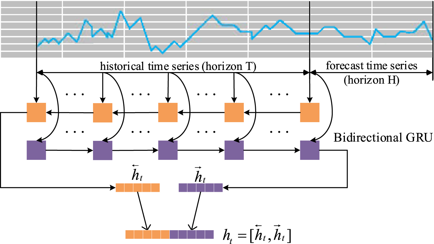
The bidirectional GRU encoder.

${\vec{h}}_{t} = \vec{GRU} ({\vec{h}}_{t - 1}, y_{t})$ (4) ${\overset{\leftarrow}{h}}_{t} = \overset{\leftarrow}{GRU} ({\overset{\leftarrow}{h}}_{t - 1}, y_{t})$ (5) The representation $h_{t} = [{\vec{h}}_{t}, {\overset{\leftarrow}{h}}_{t}]$ of each time-series record is obtained by concatenating the forward and backward hidden states from GRU networks. With the bidirectional GRU, we can encode both past and future information in representation h_t, which is useful for forecasting. In all the experiments, the encoded time-series data are used as initial inputs of our models.

4.3 Meta training

Meta-training is our model training mechanism for few-shot time series tasks. The overall procedure of meta-training is shown in Fig. 2, where steps 0-7 train model on training task-sets D_T to learn and generalize the meta-knowledge that can help model quickly adapt to new tasks. The first-order MAML algorithm is the core component in meta-training phase. The support set and query set mentioned below refer to training set and testing set of the task respectively, and more details with training datasets can be found in Section 5.1.

Fig. 2

Meta-training and Meta-testing learning mechanism.

Formally, we define Meta_model = {Meta₁, Meta₂, …} where each model has corresponding parameter vector θ_{Meta_model} = { θ_Meta₁ , θ_Meta₂ , …, }. In our experimental setups, Meta_model consists of three DNN-based models, i.e., Meta_model = {M-CNN, M-LSTM, M-CCL}, θ_{Meta_model} = { θ_M-CNN , θ_M-LSTM , θ_M-CCL }, and more details with the experimental models can be found in Section 5.2. For simplicity of notation, the following description uses M-CNN as an example, and other Meta_i ∈ Meta_model have the same process. Among the whole training mechanism, step 0 initializes M-CNN by random parameter vector θ , i.e., θ_M-CNN ← θ , and then step 1 copies θ_M-CNN to TaskNet and MetaNet, where both the TaskNet and the MetaNet are neural networks with the same structure as M-CNN, and TaskNet has parameter vector θ_t . The f_{θ_t} is a parameterized function with the parameter vector θ_t . Step 2 performs sampling from the training tasks-set D_T. Step 3 updates parameter vector θ_t through calculating the loss $L_{T_{i} \in D_{T}}^{S_{i}} (f_{θ_{t}})$ on the support set S_i of training task T_i ∈ D_T in the current episode, which is shown in Eq. (6) where the step size α is a fixed hyper-parameter. Step 4 only uses TaskNet to calculates loss $L_{T_{i}}^{Q_{i}} (f_{θ_{t}})$ on query set Q_i but not to update parameter vector θ_t . $θ_{t} \leftarrow θ_{t} - α \nabla_{θ_{t}} L_{T_{i} \in D_{T}}^{S_{i}} (f_{θ_{t}})$ (6)

Since there may be more than one sampling task in step 2, Eq. (6) could be performed several times to update the parameter vector θ_t . After the TaskNet updates in the current episode, the loss L_Q, a sum loss on the query set of all the sampling tasks, i.e., Q = {Q₁, Q₂, …} is calculated by Eq. (7). $L_{Q} = \sum_{T_{i} \in D_{T}} L_{T_{i}}^{Q_{i}} (f_{θ_{t}})$ (7) Step 5 is a core component in meta-training phase. It calculates the gradients on L_Q to update the parameter vector θ_m of MetaNet, which is shown in Eq. (8) where the step size β is a fixed hyper-parameter. Eq. (9) can be obtained by applying Eq. (7) to Eq. (8). $θ_{m} \leftarrow θ_{m} - β \nabla_{θ_{m}} L_{Q}$ (8) $θ_{m} \leftarrow θ_{m} - β \nabla_{θ_{m}} \sum_{T_{i} \in D_{T}} L_{T_{i}}^{Q_{i}} (f_{θ_{t}})$ (9)

The cycle in step 6 proceeds to the next episode until the termination condition is met. Eq. (10) shows the general learning objective of meta-training. Step 7 obtains meta-knowledge ω^* from MetaNet. In our method, the ω^* is parameter vector θ_m of MetaNet, which would be assigned to M-CNN. $ω^{*} = arg max_{ω} log p (ω | D_{T})$ (10)

4.4 Meta testing

The goal of meta-testing is to rapidly generalize the Meta_model to target task, where a small number of samples from the target task is used to update parameters of the Meta_model through only a few iterations to prevent overfitting. Steps 8 and 9 utilize meta-knowledge ω^* and the small number of samples S from the target task to fine-tune the M-CNN. The general learning objective of meta-testing is formalized in Eq. (11), where $T_{target}^{S}$ represents the support set of the target task and the θ^* is the best parameter vector for the model. Compared with the first-order MAML, instead of directly using the step size α of TaskNet in Step 9, we introduce a new step size γ during fine-tuning phase to finely control over the training process, which is shown in Eq. (12) where the $L_{T_{target}^{S}}$ is the loss function of Meta_model in the support set of the target task. In step 10, the performance of M-CNN is evaluated by calculating the evaluation metrics on the query set of the target task. $θ^{*} = arg max_{θ} log p (θ | ω^{*}, T_{target}^{S})$ (11) $θ \leftarrow θ - γ \nabla_{θ} L_{T_{target}^{S}} (f_{θ})$ (12)

5 Experimental evaluation

5.1 Datasets

In this work, we have selected 13 publicly available datasets of different domains and one Electricity Power dataset to evaluate the proposed method. Table 1 shows the attributes of each dataset in detail.

Table 1
Datasets from UCR Time Series Archive used for the experimental study, Columns N, length refer to the number of time series, time series length respectively

ID datasets N length data source

1 Beef 60 470 UCR Time Series Archive [36, 37]

2 BeetleFly 40 512

3 BirdChicken 40 470

4 Car 120 577

5 Coffee 56 286

6 FaceFour 112 350

7 Herring 128 512

8 Lighting2 121 637

9 Lighting7 143 319

10 Meat 120 448

11 OliveOil 60 570

12 Rock 70 2844

13 Wine 111 234

ID	datasets	N	length	data source
1	Beef	60	470	UCR Time Series Archive [36, 37]
2	BeetleFly	40	512
3	BirdChicken	40	470
4	Car	120	577
5	Coffee	56	286
6	FaceFour	112	350
7	Herring	128	512
8	Lighting2	121	637
9	Lighting7	143	319
10	Meat	120	448
11	OliveOil	60	570
12	Rock	70	2844
13	Wine	111	234

The datasets from UCR Time Series Archive . The UCR Time Series Archive [36, 37], introduced in 2002, is an important resource in the time series data mining community. The latest expansion version of UCR includes 128 datasets. We omit datasets that either contain missing values, or the number of time series more than 200 records. Then we obtain 13 datasets with different domains as 13 tasks. Figure 3 displays some instances of datasets from UCR Time Series Archive, in which each subfigure is from a dataset, and the red and blue curves in subfigure represent two time-series instances. A clear point via observing Fig. 3 is that the time-series instances from different datasets have significant difference.

Fig. 3

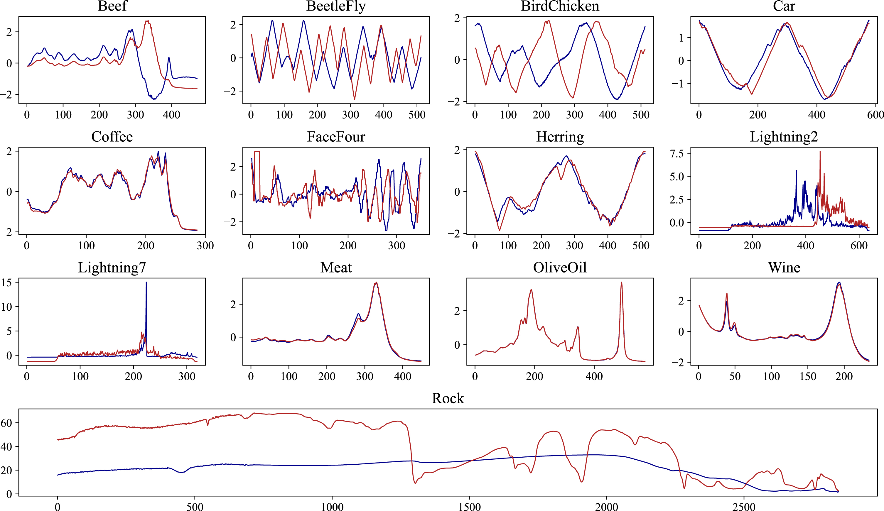
Time series instances for each dataset from UCR Time Series Archive.

Electricity Power . The dataset is about electric heating energy consumption from State Grid in Northeast China. The detailed information about the dataset can be found in Table 2. The dataset has a wide range of consumers, including hospitals, schools, government departments, factories, communities and commercial consumers. The electricity consumption habits of different consumers are obviously different. Figure 4(a) illustrates the situation, and each instance represents a typical daily load curve for one consumer. In addition, electric heating data is extremely volatile due to the economic cost, there are significant differences in typical daily load curves even for the same type of consumers. In Fig. 4(b), the time-series for “0009” and “0010” consumers are both from ordinary industry, however, there are clear differences between the two curves. The consumer “0009” uses electricity almost all day, but the consumer “0010” only uses electricity at night. Therefore, we obtain 106 tasks according to different consumers.

Fig. 4

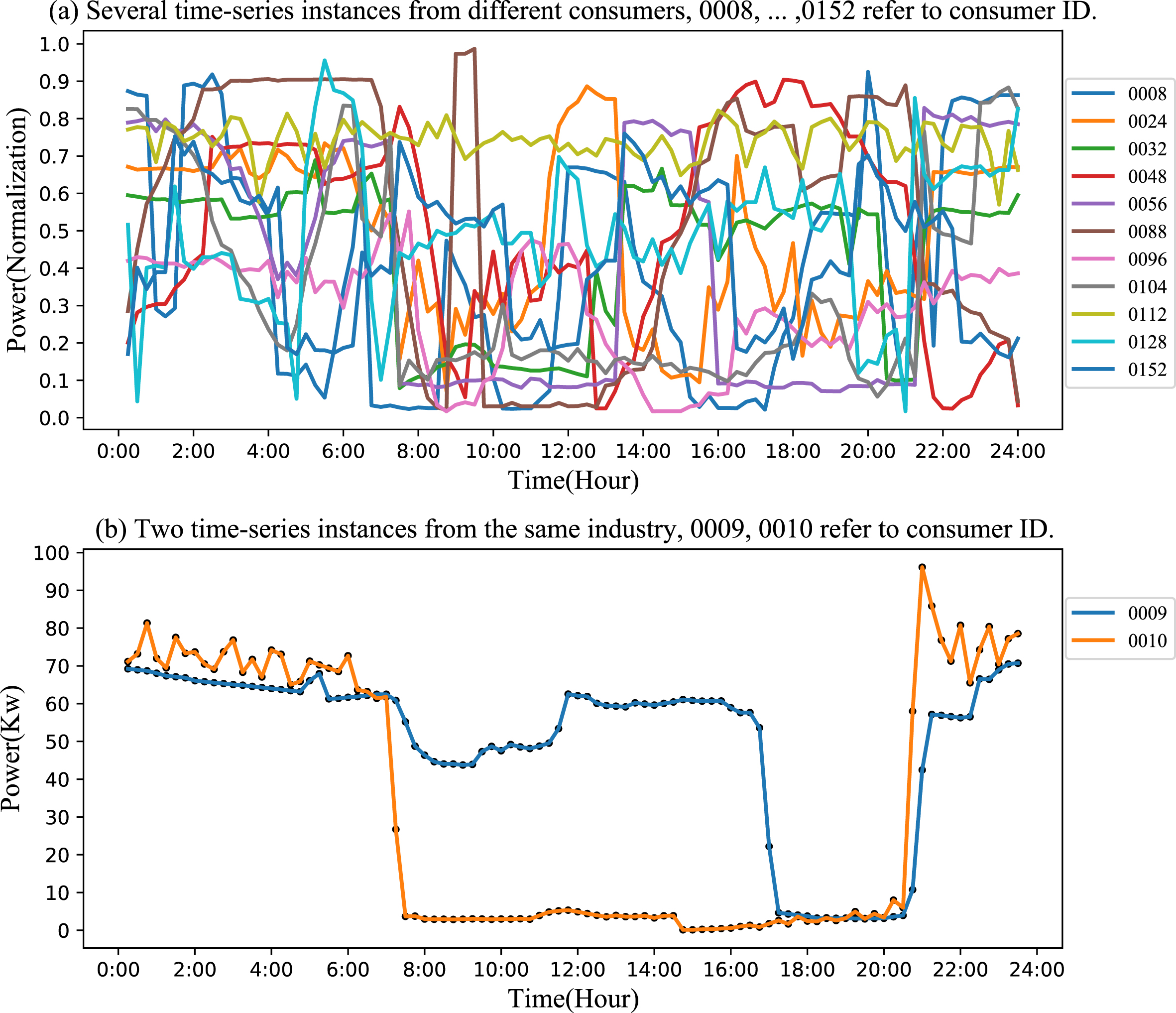
Time series instances from Electricity Power dataset.

Table 2

Electricity Power dataset used for the experimental study, Columns Min-N, Max-N respectively refer to maximum and minimum number of time series records among all consumers

consumer	Min-N	Max-N	length
106	51	91	96

5.2 Baseline models

A recent comprehensive review [33] about using deep learning techniques for time series forecasting refers to that long short-term memory (LSTM) and convolutional neural networks (CNN) are the best alternatives among all studied models, including multi-layer perceptron (MLP), Elman recurrent neural network, LSTM, echo state network, GRU, CNN and temporal convolutional network (TCN). Therefore, the LSTM, CNN, are selected as baseline models in our experiments. In addition, a hybrid model of CNN concatenating LSTM (CCL) is also selected as one of baseline model in our experiments. Additionally, complex models are likely to suffer from overfitting problem, therefore a simple multi-layer perceptron (MLP) also is selected as baseline model in our experiments.

In this paper, two groups of comparison models are designed to validate the effectiveness of the proposed method. The first group is called Base_model, including B-CNN, B-LSTM, B-CCL, which is trained directly on time-series dataset from target task, and the second is called Meta_model, including M-CNN, M-LSTM, and M-CCL, which is trained using our proposed method. Also, we supplement a group of contrast experiment between Meta_model and MLP to compare the performance difference between Meta_model and simple model on few-shot scenario.

MLP Multi-Layer Perceptron (MLP) is the most basic type of feed-forward artificial neural network. Its architecture consists of a three-block structure: an input layer, hidden layers, and an output layer, in which the number of hidden layers determines the depth of network.

CNN The typical architecture of CNN generally consists of the convolution layer, pooling layer, and fully connected layer, which is originally employed to extract multi-level feature maps and then to solve relevant downstream tasks in the field of computer vision. Sequence data can be regarded as one-dimensional image from topology, so some works [14, 34] utilize CNN to deal with time series forecasting task.

LSTM The LSTM model is one of the well-known architecture in the family of recurrent neural networks. It has solved the memory-forgetting problem that exists in vanilla RNN very well due to its special gate-controlled and information flow mechanism, such that it is frequently used in dealing with sequence data. The core of the LSTM is the cell state throughout the whole model, and the flow and change of information in the cell state are determined by a special gate-controlled mechanism. Since LSTM is naturally suitable for sequence data, quite a few relevant studies [13, 35] for time series forecasting problems can be found.

CCL Due to the powerful representation capacity of both CNN and LSTM, a hybrid model that CNN concatenate LSTM (CCL) is natural idea. In our experiment, the part of CNN is treated as feature extractor and the part of LSTM is used to capture underlying temporal features.

5.3 Training setups

The datasets from UCR Time Series Archive have split standard train set and test set, therefore, we split Electricity Power dataset according to tasks into train and test subsets with approximate scale. Table 3 shows detailed training and testing scales used time-series data in experiments.

Table 3
Details of the time series data used in training and testing phase, Column Task N refer to the number of tasks, Column Min-N, Max-N refer to the minimum and maximum number of time-series records among all tasks in the training phase respectively, and Column Train ST, Test ST refer to the number of all time-series records used in training and testing phases respectively

Task N Min-N Max-N Train ST Test ST

119 20 70 4199 4367

Task N	Min-N	Max-N	Train ST	Test ST
119	20	70	4199	4367

For each task, we set four different forecast horizons (H = 10, 20, 30, 40) to check the robustness of the proposed method. Since time series forecasting is a typical regression task, the model parameters are updated by minimizing the MSE (Mean Square Error) loss: $Loss = \frac{1}{H} \sum_{i = 1}^{H} (y_{T + i} - {\hat{y}}_{T + i})^{2}$ (13)Base_model are trained directly using time-series dataset from target task. Since the scale of training set for single task is quite small (no more than 70 records), the model updates parameters once until all time-series data from the task are input. We use the train set to tune learning rate. Some other hyper-parameters, like the convolutional kernel of CNN, the hidden size of LSTM units, are not finely selected. There may be better configurations available, but that is not the focus of this work. Please refer to the supplement for detailed hyper-parameter settings.

For Meta_model, we split training tasks-set and target task for cross-task learning, which is expected to be able to generalize some transferable knowledge to achieve rapid adaptation on target task. The specific splitting way is that one task is selected as target task and the rest as training tasks-set. Therefore, the size of training tasks-set is 118. For each task, the training set and testing set are treated as support set and query set respectively in this phase. The learning rate of meta-training phase is fine-tuned by support and query set, and the learning rate γ of meta-testing phase is the same with training process of Base_model. Other model hyper-parameters are the same with Base_model. Please refer to supplement for detailed hyper-parameter settings.

5.4 Experimental results

Figure 5 studies the difference of sMAPE between Meta_model and Base_model on four different forecast horizons for all tasks. X-axis represents different tasks, and Δ-sMAPE means sMAPE(Base_model) minus sMAPE(Meta_model). Δ-sMAPE is greater than zero, which means that the performance of Meta_model has been improved compared with Base_model. Figure 5 illustrates that compared with Base_model, Meta_model has a significant performance improvement on most tasks, with only a few tasks showing performance drop. Figure 6 studies the difference of RMSE between Meta_model and Base_model on four different forecast horizons for all tasks. Figure 6 shows that M-CNN in all configurations achieves significant RMSE’s decrease on some tasks and the increase of RMSE is occurred only on a small number of tasks, however, for M-LSTM and M-CCL, the task proportion with increased and decreased RMSE is very close on some configurations. For the phenomenon, a reasonable explanation is that M-LSTM and M-CCL have a more complex neural network architecture compared with M-CNN, thus they suffer relatively stronger overfitting in the meta-testing phase. Table 4, 5 clearly confirms the above conclusion with statistics. However, a reasonable question for the comparison results obtained above is whether the Base_model suffer from overfitting problem in the training phase such that the Meta_model look like achieving a better performance compared with Base_model. With this question, we supplement a group of contrast experiment on a simple MLP model, and the model has only one hidden layer with 100 neurons. Table 6, 7 show the proportion of tasks with performance improvement and degradation among all tasks for Meta_model compared with MLP in terms of sMAPE and RMSE, respectively. Experimental results indicate that Meta_model have better performance than the MLP model on majority of tasks under four different forecast horizons, which not only solves the aforementioned question but demonstrates the effectiveness of Meta_model again. Note that the percentages beside the up and the down arrows in Table 4, 5, 6, 7 represent the proportion of tasks with performance improvement and degradation, respectively, and the task will be counted when the absolute difference between Meta_model and Base_model is greater than 0.1. Therefore, the sum of the up and the down percentages may not equal 1 in Table 4, 5, and the remaining percentages represent that the differences between Meta_model and Base_model are not significant. A more detailed analysis and experimental result of RMSE are provided in supplement.

Fig. 5

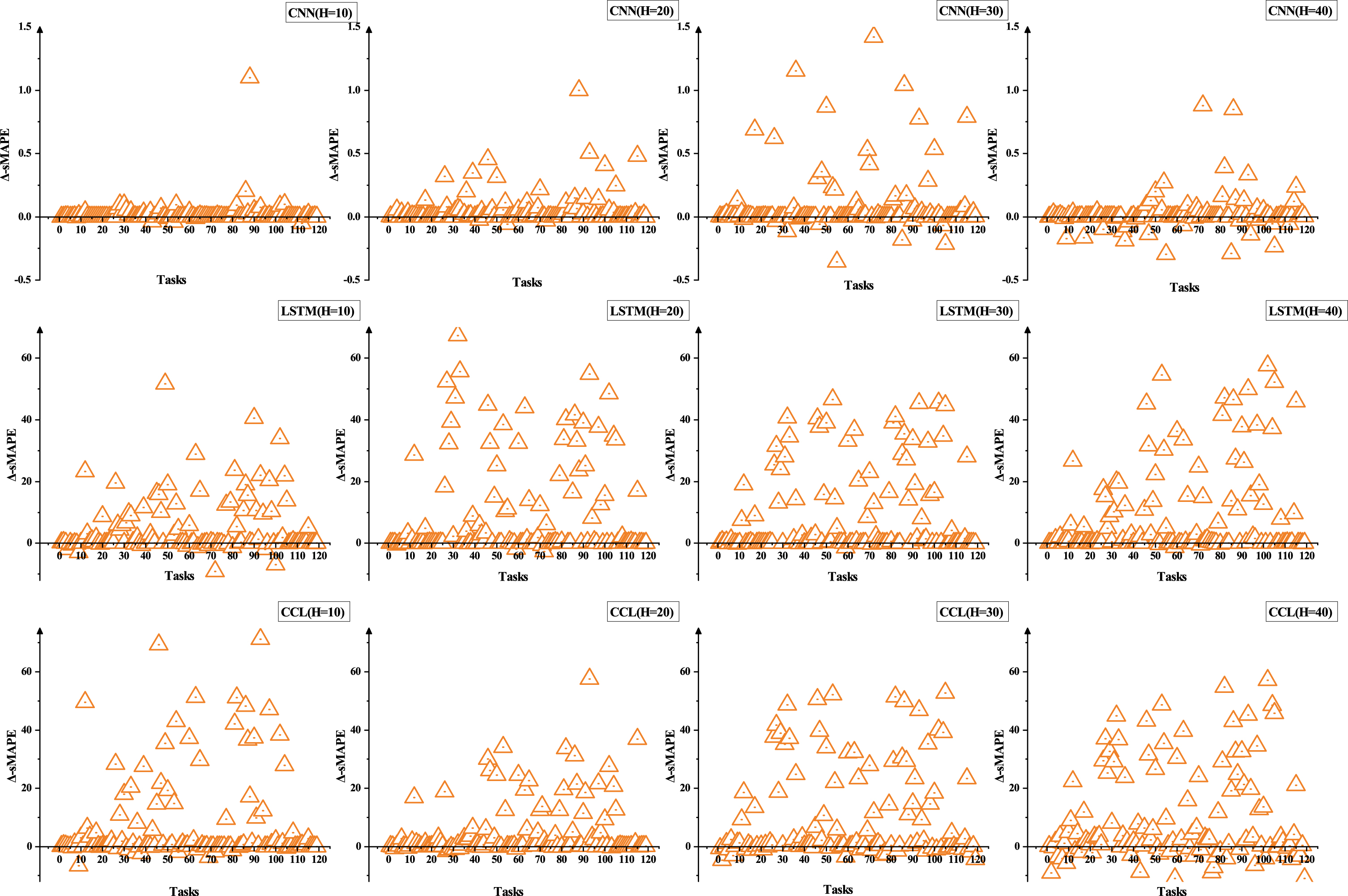
The comparison of sMAPE between Base_model and Meta_model, Δ-sMAPE means sMAPE(Base_model) minus sMAPE(Meta_model).

Fig. 6

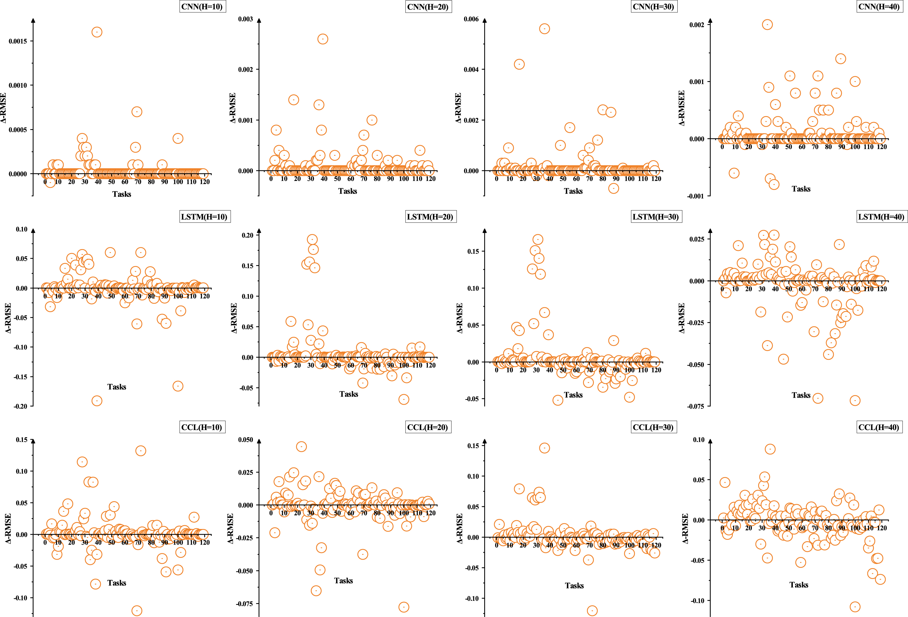
The comparison of RMSE between Base_model and Meta_model, Δ-RMSE means RMSE(Base_model) minus RMSE(Meta_model).

Table 4

The proportion of tasks with performance improvement and degradation among all tasks on sMAPE for Meta_model

	H=10	H=20	H=30	H=40
CNN	(42.86% ↑) (6.72% ↓)	(55.46% ↑) (3.36% ↓)	(48.74% ↑) (12.61% ↓)	(69.75% ↑) (26.05% ↓)
LSTM	(73.95% ↑) (26.05% ↓)	(84.03% ↑) (15.13% ↓)	(84.87% ↑) (15.13% ↓)	(94.12% ↑) (5.88% ↓)
CCL	(62.18% ↑) (36.13% ↓)	(73.11% ↑) (26.89% ↓)	(70.59% ↑) (29.41% ↓)	(68.07% ↑) (31.93% ↓)

Table 5

The proportion of tasks with performance improvement and degradation among all tasks on RMSE for Meta_model

	H=10	H=20	H=30	H=40
CNN	(16.81% ↑) (0.84% ↓)	(28.57% ↑) (0.00% ↓)	(24.37% ↑) (3.36% ↓)	(28.57% ↑) (5.04% ↓)
LSTM	(40.34% ↑) (44.54% ↓)	(45.38% ↑) (37.82% ↓)	(49.58% ↑) (35.29% ↓)	(58.82% ↑) (32.77% ↓)
CCL	(45.38% ↑) (46.22% ↓)	(46.22% ↑) (44.54% ↓)	(41.18% ↑) (58.82% ↓)	(47.90% ↑) (52.10% ↓)

Table 6

The proportion of tasks with performance improvement and degradation among all tasks on sMAPE for Meta_model compared with MLP

	H=10	H=20	H=30	H=40
M-CNN	(68.91% ↑) (18.49% ↓)	(77.31% ↑) (11.76% ↓)	(84.03% ↑) (5.88% ↓)	(88.24% ↑) (5.04% ↓)
M-LSTM	(72.27% ↑) (15.97% ↓)	(80.67% ↑) (8.40% ↓)	(84.03% ↑) (4.20% ↓)	(91.60% ↑) (2.52% ↓)
M-CCL	(75.63% ↑) (14.29% ↓)	(81.51% ↑) (9.24% ↓)	(60.50% ↑) (30.25% ↓)	(50.42% ↑) (49.58% ↓)

Table 7

The proportion of tasks with performance improvement and degradation among all tasks on RMSE for Meta_model compared with MLP

	H=10	H=20	H=30	H=40
M-CNN	(5.04% ↑) (0.84% ↓)	(1.68% ↑) (0.84% ↓)	(0.84% ↑) (0.00% ↓)	(0.84% ↑) (0.84% ↓)
M-LSTM	(3.06% ↑) (0.00% ↓)	(5.88% ↑) (0.00% ↓)	(5.88% ↑) (0.00% ↓)	(0.84% ↑) (0.00% ↓)
M-CCL	(5.88% ↑) (0.00% ↓)	(0.84% ↑) (0.00% ↓)	(1.68% ↑) (0.00% ↓)	(0.84% ↑) (0.84% ↓)

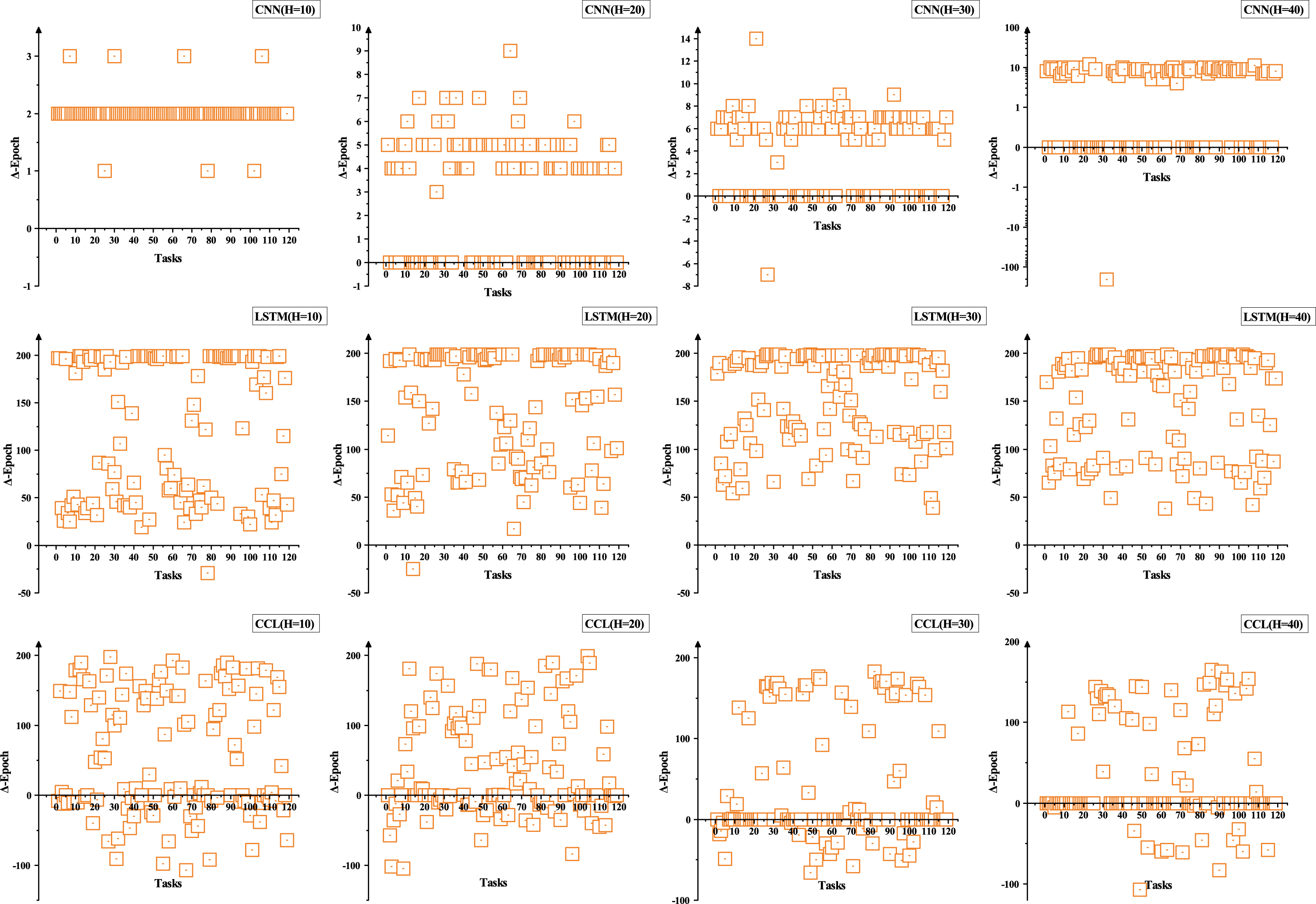
Figure 7 compares convergence epochs between Meta_model and Base_model on four different forecast horizons for all tasks. Δ-Epoch means that Epoch(Base_model) minus Epoch(Meta_model). It can be found that Meta_model converges faster than Base_model for most tasks, which means that Meta_model can adapt to target task more quickly than Base_model. Therefore, our method alleviates the overfitting problem of DNN-based models in few-shot scenarios. Note that in meta-testing phase, Meta_model have exactly the same experimental settings with Base_model, including model architecture, optimizer, learning rate, etc. In Table 8, the percentages beside the up arrow represent the proportion of tasks with faster convergence speed and no degradation of sMAPE, and beside the down arrow represent the proportion of tasks with degradation in both sMAPE and converge speed. Table 8 clearly confirms that the proposed method converges faster while no negative impact for model performance on most tasks, which effectively alleviates the overfitting problem that tends to occur in few-shot scenarios.

Fig. 7

The comparison of Convergence Epochs between Base_model and Meta_model, Δ-Epoch refers to Epoch(Base_model) minus Epoch(Meta_model).

Table 8

The proportion of tasks with convergence speed up and down among all tasks for Meta_model

	H=10	H=20	H=30	H=40
CNN	(93.28% ↑) (0.00% ↓)	(57.14% ↑) (0.00% ↓)	(49.58% ↑) (0.84% ↓)	(34.45% ↑) (0.84% ↓)
LSTM	(73.95% ↑) (0.84% ↓)	(84.87% ↑) (0.84% ↓)	(84.87% ↑) (0.00% ↓)	(94.12% ↑) (0.00% ↓)
CCL	(50.42% ↑) (23.53% ↓)	(50.42% ↑) (17.65% ↓)	(38.66% ↑) (7.56% ↓)	(30.25% ↑) (4.20% ↓)

Figure 8 depicts the change in performance of the different Meta_model on all tasks with the increase of forecast horizon, in which the performance of Meta_model does not obviously fluctuate as the forecast horizon changes, and tends to improve in terms of the overall trend. It demonstrates the proposed method is strongly robust for the growth of forecast horizon.

Fig. 8

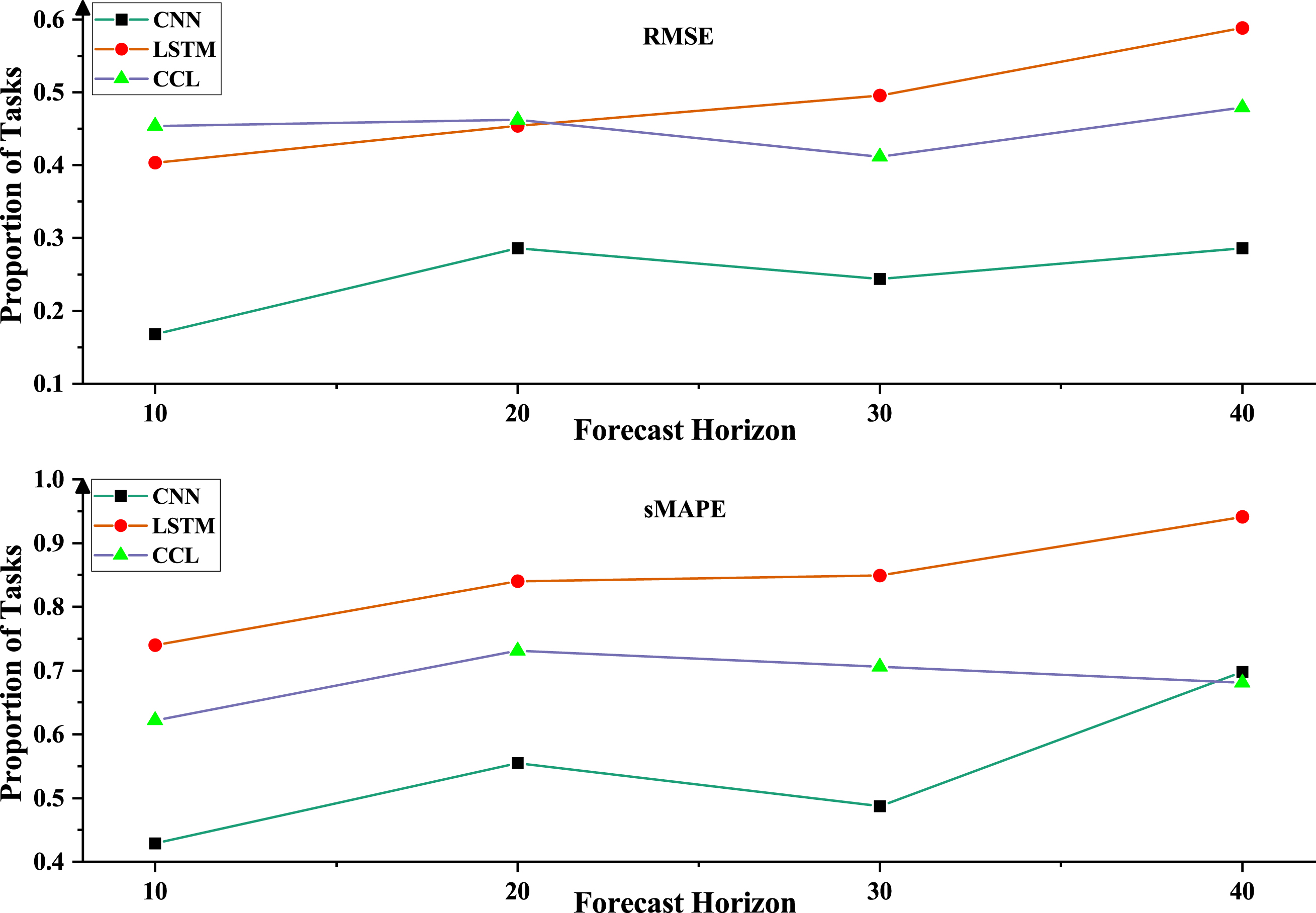
The proportion of tasks with improved performance among all tasks on four different forecast horizons.

5.5 Statistical analysis

We perform the statistical tests for all models used in experiments, grouping the results according to different forecast horizons with respect to ranking of sMAPE. In all cases, the p-value obtained in the Friedman test denotes that null hypothesis is rejected, which indicates that the performance differences in ranking among all models is significant. Therefore, we proceed with a post-hoc analysis based on the Wilcoxon-Holm method to perform a pairwise comparison between the models. Figure 9 displays the ranking of models from left to right on sMAPE for four different forecast horizons, and the horizontal lines linking the models indicate that it is hard to detect differences between models with similar performance in this scenario. In this critical differences diagram, Meta_model show a consistent superior rank compared with counterparts in Base_model. Furthermore, we can find the M-LSTM and M-CNN displays superior performance in all forecast horizons, and B-CNN also has a better rank compared with other Base_model even surpasses M-CCL when forecast horizon is 30 and 40. A reasonable explanation is that B-CNN has a simpler architecture compared with other Base_model, thus B-CNN suffers relatively weak overfitting when the training data is quite small.

Fig. 9

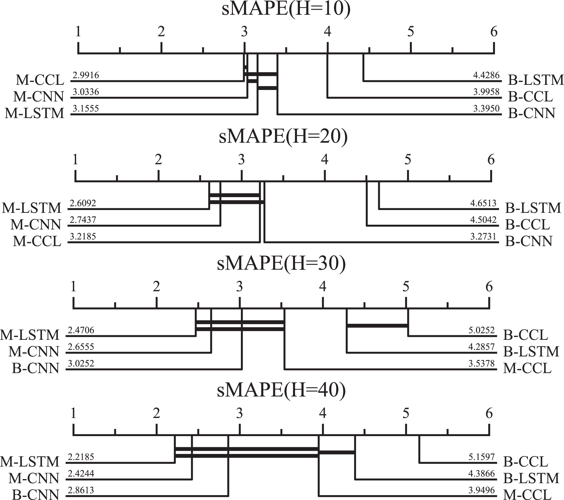
Ranking and critical differences diagram (using the Wilcoxon-Holm method) of the performance metric sMAPE on all tasks, significant level for Friedman test is set 0.05.

5.6 Data sensitivity study

Although Section 5 mentions that the tasks from Electricity Power dataset are quite different, it is a fact that cannot be ignored that nearly 90% of the tasks used in experiments are from the Electricity Power dataset. An obvious question is that whether the experimental results obtained are affected by skewed data. With this question, we proceed with data sensitivity study. Table 9 shows the detailed data information used for the study. The training tasks-set consists of all tasks in UCR Archive and three randomly selected tasks from Electricity Power dataset.

Table 9
Details of the time series data used in data sensitivity study, Column Train Min-N, Train Max-N refer to the minimum and maximum number of time-series records among all tasks respectively, and Column Train ST, Test ST refer to the number of all time-series records used in training and testing phases respectively

Task Number Tasks from UCR Tasks from EP^a Train Min-N Train Max-N Train ST Test ST

16 13 3 20 70 630 728

Task Number	Tasks from UCR	Tasks from EP^a	Train Min-N	Train Max-N	Train ST	Test ST
16	13	3	20	70	630	728

^arefers to Electricity Power dataset.

Table 10 displays that Meta_model achieves performance improvement on four different forecast horizons compared with Base_model, and there is no significant performance degradation on any of the tasks used in data sensitivity study. Note that the arrows in Table 10 have the same meaning as those in Table 4. Experimental results on convergence speed of models for data sensitivity study can be found in supplement. Furthermore, the statistical tests also are performed. Figure 10 depicts the ranking of models from left to right on sMAPE for four different forecast horizons. In Fig. 10, a similar conclusion can be found with Fig. 9, i.e. Meta_model show a consistent superior rank compared with counterparts in Base_model and B-CNN has a better rank compared with other Base_model. The above results at least demonstrate two properties: (1) probable data skewing does not significantly affect the experimental conclusions obtained, and (2) the performance of Meta_model does not obviously fluctuate when the scale of the dataset used changes significantly.

Table 10

The proportion of tasks with performance improvement and degradation on sMAPE for Meta_model

	H=10	H=20	H=30	H=40
CNN	(6.25% ↑) (0.00% ↓)	(6.25% ↑) (0.00% ↓)	(18.75% ↑) (0.00% ↓)	(18.75% ↑) (0.00% ↓)
LSTM	(62.50% ↑) (0.00% ↓)	(68.75% ↑) (0.00% ↓)	(56.25% ↑) (0.00% ↓)	(56.25% ↑) (0.00% ↓)
CCL	(56.25% ↑) (0.00% ↓)	(56.25% ↑) (0.00% ↓)	(87.50% ↑) (0.00% ↓)	(1.00% ↑) (0.00% ↓)

Table 11

The proportion of tasks with convergence speed up and down for Meta_model

	H=10	H=20	H=30	H=40
CNN	(56.25% ↑) (0.00% ↓)	(50.00% ↑) (0.00% ↓)	(56.25% ↑) (0.00% ↓)	(50.00% ↑) (0.00% ↓)
LSTM	(93.75% ↑) (0.00% ↓)	(1.00% ↑) (0.00% ↓)	(1.00% ↑) (0.00% ↓)	(93.75% ↑) (0.00% ↓)
CCL	(68.75% ↑) (0.00% ↓)	(87.50% ↑) (0.00% ↓)	(93.75% ↑) (0.00% ↓)	(1.00% ↑) (0.00% ↓)

Table 12

Hyper-parameter configurations for training of Base_model on all tasks

	CNN	LSTM	CCL
Learning Rate	0.5	0.1	0.01
Epoch	500	200	200

Table 13

Hyper-parameter configurations on Meta-training phase for all tasks

	CNN	LSTM	CCL
α	0.1	0.001	0.001
β	0.5	0.5	0.5
Number of Samples	5	5	5
Multiple Gradient Updates	5	5	5

Fig. 10

Ranking and critical differences diagram (using the Wilcoxon-Holm method) of the performance metric sMAPE for data sensitivity study, significant level for Friedman test is set 0.05.

Fig. 11

The comparison of RMSE among B-CNN, B-LSTM and B-CCL for four different forecast horizons.

6 Conclusion

In this paper, we focus on few-shot time series forecasting problems and propose employing meta-learning techniques to obtain valid and transferrable knowledge by cross-task training. Due to inconsistent time series length of cross-domain data, a shared encoder (BiGRU) is used to encode time-series records to a unified dimension. We select three DNNs architectures with superior performance on time series forecasting tasks as baseline models and design two groups of comparison models, including Meta_model and Base_model. Base_model is trained on specific time-series dataset for each target task. For Meta_model, we propose employing meta-training to learn transferable meta-knowledge from different time series tasks and meta-testing to perform fine-tuning on specific target task.

Extensive experimental results and analysis allow us to draw the following conclusions: (1) the performance of Meta_model outperforms the Base_model on most tasks, which indicate that Meta_model successfully generalize transferable features that are conducive to cope with few-shot scenarios by cross-task learning on meta-training phase, (2) benefitting from the training mechanism of first-order MAML algorithm, Meta_model has a faster convergence speed on meta-testing phase and without occurring performance degradation on most tasks, which largely alleviates the overfitting problems of DNN-based model in few-shot scenarios, (3) the proposed method has strong robustness for forecast horizons and data scales.

We also noticed that Meta_model occurred performance degradation of different degree in our experiments. Specifically, with the increase of model’s complexity, the task ratio of performance degradation also tends to rise. For the phenomenon, we speculate that overfitting problem in some tasks dominates the model’s performance with the increase of model’s complexity. As for the Meta_model used in this work, like M-LSTM and M-CCL, introducing regularization term to loss function is a promising solution to alleviate the overfitting problem. In addition, we expect to solve the problem in the future work via designing new neural network architecture as low-complexity as possible according to the inner features of time-series data and enlarging the task scale of cross-task training.

In the interest of reproducibility, the detailed hyper-parameters settings can be found in supplement, and integral experimental code is publicly available at https://github.com/2154022466/Meta-Learning4FSTSF.

Footnotes

Acknowledgment

This work is supported by the National Natural Science Foundation of China under grant No.61872163 and 61806084, Jilin Provincial Education Department project under grant No. JJKH20190160KJ, Jilin Province Key Scientific and Technological Research and Development Project under grant No. 20210201131GX, and the State Grid Corporation of China Technology Project under grant No. 522300190009.

Supplement

Figure 11 depicts the comparison of RMSE among B-CNN, B-LSTM and B-CCL for four different forecast horizon configurations. In Fig. 11, We can see that the RMSE of B-CNN is very close to that of B-LSTM and B-CCL on all tasks, which indicates that B-CNN has comparable performance with B-LSTM and B-CCL. This demonstrates M-CNN in gets a performance improvement not because B-CNN is a weak model.

Table 11 shows Meta_model converges faster on most tasks used for data sensitivity study compared with Base_model, and there is no occurring simultaneous degradation of model performance and convergence speed. Note that the arrows in Table 11 have the same meaning as those in .

Hyper-parameter settings

All models used in experiments are trained on one machine with 1 NVIDIA RTX 2080Ti GPU.

References

, Yu

, Shahabi

and Liu

, Diffusion Convolutional Recurrent Neural Network: Data-Driven Traffic Forecasting, 6th International Conference on Learning Representations, Vancouver, May 2018.

Laptev

, Yosinski

, Li

L.E.

and Smyl

, Time-series extreme event forecasting with neural networks at uber, International Conference on Machine Learning 34 (2017), 1–5.

Ruiz

L.G.B.

, Rueda

, Cuéllar

M.P.

and Pegalajar

M.C.

, Energy consumption forecasting based on Elman neural networks with evolutive optimization, Expert Systems with Applications 92 (2018), 380–389.

Deb

, Zhang

, Yang

, Lee

S.E.

and Shah

K.W.

, A review on time series forecasting techniques for building energy consumption, Renewable and Sustainable Energy Reviews 74 (2017), 902–924.

Sharma

R.R.

, Kumar

, Maheshwari

and Ray

K.P.

, EVDHM-ARIMA-Based Time Series Forecasting Model and Its Application for COVID-19 Cases, IEEE Transactions on Instrumentation and Measurement 70 (2021), 1–10.

Henrique

B.M.

, Sobreiro

V.A.

and Kimura

, Literature review: Machine learning techniques applied to financial market prediction, Expert Systems with Applications 124 (2019), 226–251.

Box

and Jenkins

, Time Series Analysis: Forecasting and Control, Journal of the American Statistical Association, 1990.

Van Gestel

, et al., Financial time series prediction using least squares support vector machines within the evidence framework, IEEE Transactions on Neural Networks 12(4) (2001), 809–821.

H.F.

, Rao

and Dhillon

I.S.

, Temporal Regularized Matrix Factorization for High-dimensional Time Series Prediction, Advances in Neural Information Processing Systems 29 (2016), 847–855.

10.

Krizhevsky

, Sutskever

and Hinton

G.E.

, Imagenet classification with deep convolutional neural networks, Advances in Neural Information Processing Systems 25 (2012), 1097–1105.

11.

, Zhang

, Ren

and Sun

, Deep Residual Learning for Image Recognition, Proceedings of the IEEE Conference on Computer Vision and Pattern Recognition, 2016, pp. 770–778.

12.

Sutskever

, Vinyals

and Le

Q.V.

, Sequence to Sequence Learning with Neural Networks, Advances in Neural Information Processing Systems 27 (2014), 3104–3112.

13.

Sagheer

and Kotb

, Time series forecasting of petroleum production using deep LSTM recurrent networks, Neurocomputing 323 (2019), 203–213.

14.

Cai

, Pipattanasomporn

and Rahman

, Dayahead building-level load forecasts using deep learning vs. traditional time-series techniques, Applied Energy 236 (2019), 1078–1088.

15.

Borovykh

, Bohte

and Oosterlee

, Dilated convolutional neural networks for time series forecasting, Journal of Computational Finance 22(4) (2019), 73–101.

16.

Akaike

, Fitting autoregressive models for prediction, Annals of the institute of Statistical Mathematics 21(1) (1969), 243–247.

17.

Ulrych

T.J.

and Clayton

R.W.

, Time series modelling and maximum entropy, Physics of the Earth and Planetary Interiors 12(2-3) (1976), 188–200.

18.

Friston

K.J.

, Williams

, Howard

, Frackowiak

R.S.

and Turner

, Movement-related effects in fMRI time-series, Magnetic Resonance in Medicine 35(3) (1996), 346–355.

19.

Contreras

, Espinola

, Nogales

F.J.

and Conejo

A.J.

, ARIMA models to predict next-day electricity prices, IEEE Transactions on Power Systems 18(3) (2003), 1014–1020.

20.

Williams

B.M.

and Hoel

L.A.

, Modeling and forecasting vehicular traffic flow as a seasonal ARIMA process: Theoretical basis and empirical results, Journal of Transportation Engineering 129(6) (2003), 664–672.

21.

Zhang

G.P.

, Time series forecasting using a hybrid ARIMA and neural network model, Neurocomputing 50 (2003), 159–175.

22.

Claveria

and Torra

, Forecasting tourism demandto Catalonia: Neural networks vs. time series models, Economic Modelling 36 (2014), 220–228.

23.

Makridakis

, Spiliotis

and Assimakopoulos

, The M4 Competition: Results, findings, conclusion and way forward, International Journal of Forecasting 34(4) (2018), 802–808.

24.

Oreshkin

B.N.

, Carpov

, Chapados

and Bengio

, N-BEATS: Neural basis expansion analysis for interpretable time series forecasting, 8th International Conference on Learning Representations, Addis Ababa, April 2020.

25.

Orozco

B.P.

and Roberts

S.J.

, Zero-shot and few-shot time series forecasting with ordinal regression recurrent neural networks, 28th European Symposium on Artificial Neural Networks, Computational Intelligence and Machine Learning, Bruges, October 2020.

26.

Iwata

and Kumagai

, Few-shot Learning for Time-series Forecasting, unpublished, CoRR. Available: https://arxiv.org/abs/2009.14379

27.

Oreshkin

B.N.

, Carpov

, Chapados

and Bengio

, Meta-learning framework with applications to zero-shot time-series forecasting, Proceedings of the AAAI Conference on Artificial Intelligence (2021), pp. 9242–9250.

28.

Munkhdalai

and Yu

, Meta networks, International Conference on Machine Learning 70 (2017), 2554–2563.

29.

Finn

, Abbeel

and Levine

, Model-agnostic meta-learning for fast adaptation of deep networks, International Conference on Machine Learning 70 (2017), 1126–1135.

30.

Hospedales

, Antoniou

, Micaelli

and Storkey

, Meta-learning in neural networks: A survey, IEEE Transactions on Pattern Analysis and Machine Intelligence (2021), pp. 1–1.

31.

Snell

, Swersky

and Zemel

R.S.

, Prototypical networks for few-shot learning, Advances in Neural Information Processing Systems 30 (2017), 4077–4087.

32.

Vinyals

, Blundell

, Lillicrap

, Kavukcuoglu

and Wierstra

, Matching networks for one shot learning, Advances in Neural Information Processing Systems 29 (2016), 3630–3638.

33.

Lara-Benitez

, Carranza-García

and Riquelme

J.C.

, An Experimental Review on Deep Learning Architectures for Time Series Forecasting, International Journal of Neural Systems 31 (2021), 1–28.

34.

Koprinska

, Wu

and Wang

, Convolutional Neural Networks for Energy Time Series Forecasting, International Joint Conference on Neural Networks (IJCNN) (2018), pp. 1–8.

35.

Pan

, Tan

, Feng

and Li

, Very Short-Term Solar Generation Forecasting Based on LSTM with Temporal Attention Mechanism, IEEE 5th International Conference on Computer and Communications (ICCC) (2019), pp. 267–271.

36.

Dau

H.A.

et al., The UCR time series archive, {IEEE/CAA Journal of Automatica Sinica 6(6) (2019), 1293–1305.

37.

Dau

H.A.

et al., The UCR time series classification archive, October 2018. Available: https://www.cs.ucr.edu/~eamonn/time_series_data_2018/