Complex-InversE: Improving bilinear knowledge graph embeddings by mapping into complex space

Abstract

Knowledge graph link prediction uses known fact links to infer the missing link information in the knowledge graph, which is of great significance to the completion of the knowledge graph. Generating low-dimensional embeddings of entities and relations which are used to make inferences is a popular way for such link prediction problems. This paper proposes a knowledge graph link prediction method called Complex-InversE in the complex space, which maps entities and relations into the complex space. The composition of complex embeddings can handle a large variety of binary relations, among them symmetric and antisymmetric relations. The Complex-InversE effectively captures the antisymmetric relations and introduces Dropout and Early-Stopping technologies into deal with the problem of small numbers of relationships and entities, thus effectively alleviates the model’s overfitting. The results of comparison experiment on the public knowledge graph datasets show that the Complex-InversE achieves good results on multiple benchmark evaluation indicators and outperforms previous methods. Complex-InversE’s code is available on GitHub at https://github.com/ZeyuMiao97/Complex-InversE.

1 Introduction

Knowledge graphs (KGs) consist of a large number of facts, where each fact is represented as a triplet (e_s, r, e_o), which e_s and e_o represent subject and object entities and r represent a relation. At present, knowledge graphs have been applied to many artificial intelligence fields such as recommender systems [1], information retrieval [2] and natural language processing [3] and are important data sources for artificial intelligence applications such as Freebase [4], Yago [5], WordNet [6].

Most of the existing knowledge graph link prediction methods use entities, relations or graph features to perform link prediction. For a given knowledge graph learning a low-dimensional representation for all entities and relations, we usually define a score function to predict the missing links. Sun et al. [7] proposed RotatE, which defines each relation as a rotation from the source entity to the target entity in the complex vector space and propose a novel self-adversarial negative sampling technique for efficiently and effectively training their model. Vashishth et al. [8] proposed InteractE, which uses three key ideas – feature permutation, a novel feature reshaping, and circular convolution for link prediction. Zhang et al. [9] proposed QuatE, which models relations as rotations in the quaternion space.

Binary relations in KGs exhibit various types of patterns: inversion, symmetry/antisymmetry and composition. In the real world, marriage is a symmetrical relation while the relation of filiation is antisymmetric; some relations are the inverse of other relations (e.g., hypernym and hyponym); and some relations can be composed by others (e.g., my father’s wife is my mother). Under ideal circumstances, embedding models applied to link prediction should be able to learn all combinations of these properties. The keystone of embedding models is to find a balance between expressiveness and parameter space size. One popular composition function for embedding models is dot product. Dot products of embeddings perform well in scale and can naturally handle both symmetry and reflflexivity of relations, even enable transitivity with an appropriate loss function. Meanwhile, the standard dot product between embeddings can be a very effective composition function if the right representation is used. However, when dot products are used to deal with the antisymmetric relationship, the parameter space of the model will inevitably expand and implied an explosion of the number of parameters, making models prone to overfifitting.

Kazemi et al. [10] proposed a knowledge graph embedding method SimplE for knowledge graph link prediction. After generating head embedding and tail embedding for each entity and scoring the triple through score function, SimplE swaps the position of head embedding and tail embedding and score the triple again, then get the average of the two scores as the final score. However, the above methods only consider the mapping of entities and relations in real space, which could cause explosive growth of model parameters and may lead to overfitting of the model. At the same time, due to the data-driven nature of entity and relation vectorization methods, if the number of a certain type of relation or entity in the training set is too small, the vector score function of this type of entity and relation may also lead to overfitting of the model.

In response to the above problems, this paper proposes a knowledge graph link prediction method in complex space, Complex-InversE. In order to alleviate the problem that dot products cannot effectively handle the antisymmetric relations, Complex-InversE maps entities and relations to both real space and complex space. When using complex vectors to model entity and relation embeddings, facts about antisymmetric relations can receive different scores depending on the ordering of the entities involved. Thus complex vectors can control the parameter scale of the model within an acceptable range while retaining the efficiency advantage of the dot product, thereby alleviating the problem that dot products cannot effectively deal with the antisymmetric relations. At the same time, for the problem of small numbers of a certain type of relation or entity, Complex-InversE introduces Dropout and Early-Stopping to avoid overfitting of the model.

Our contributions are summarized as follows:

By mapping relations and entities into complex space, Complex-InversE effectively captures antisymmetric relations while improving the dot product efficiency of the model, and avoids the explosion of the number of parameters

We introduce a new score function in complex space. By integrating the performance of Complex-InversE in real space and complex space, the score function in complex space can effectively optimize the accuracy of Complex-InversE.

Complex-InversE can effectively alleviate the overfitting of the model caused by the small number of a certain type of relation or entity by applying Dropout. The mechanism of Early-Stopping introduced enables Complex-InversE to accurately find the most suitable number of training iterations.

The rest of this article is structured as follows: we summarize related efforts in Section 2. Then we present the Complex-InversE model and introduce three key ideas complex embedding vectors, Dropout, and Early-Stopping in Section 3. We report on the experiments in Section 4 before concluding.

2 Related work

Translation-based models describe relations as translations from source entities to target entities. The key idea of the translation-based knowledge graph link prediction method is to use vectors to express the characteristics of entities and relations. TransE [11] is a representative method among translational Approaches. TransE uses the vector translation of the vector space to characterize the correlation between entities and relations. TransE is effective in handling 1-1 relations, but is not good at dealing with complex relations like N-1, 1-N, and N-N. In response to these complex relations, Wang proposed TransH [12] which obtains different representations of entities in different relations by projecting entities onto the hyperplane where the relation is located. Lin proposed TransR [13] which embeds entities and relations in different entity spaces and relation spaces, updates embeddings through translation between projected entities, and project entities into relation subspace through projection matrix in order to obtain representations of different entities in different relations.

Bilinear models product-based score functions to match latent semantics of entities and relations embodied in their vector space representations. In DisMult [14], the embeddings of each entity and each relation is defined as $v_{e} \in ℝ^{d}$ and $v_{r} \in ℝ^{d}$ with the similarity function 〈v_h, v_r, v_t〉. For DisMult, an entity uses the same embedding as head and tail, so DisMult cannot model other relations than symmetrical relations. CompleX [15] improves DisMult by mapping entities and relations into complex spaces. CompleX divides the embedding of each entity into two parts, where ${re}_{r} \in ℝ^{d}$ as the real part and ${im}_{r} \in ℝ^{d}$ as the imaginary part. The similarity function of ComplEx is defined as $Real (\sum_{j = 1}^{d} ({re}_{h} [j] + {im}_{h} [j] i) * ({re}_{r} [j] + {im}_{r} [j] i) * ({re}_{t} [j] - {im}_{t} [j] i)$ , which can be rewritten as 〈re_h, re_r, re_t〉 + 〈 re_h, im_r, im_t 〉 + 〈 im_h, re_r, im_t 〉 - 〈 im_h, im_r, re_t 〉. Different from the previous methods, RESCAL [16] models the embedding vector of relation r as $v_{r} \in ℝ^{d \times d}$ with the similarity function v_r · vec (v_h ⊗ v_t) where ⊗ represents the vector product of two vectors and vec (.) represents vectorization of the input matrix.

Neural-Network-based Models aim to learn a neural network, to automatically model the interaction. Adding neural network to knowledge graph is a new and effective method. ConvE [17] designs a fast computational 2D convolutional neural network for the representation learning of knowledge graph. However, ConvE only considers the relations of local different dimensions but does not consider the relations of the global same dimension. ConvKB [18] convolves all three elements of the triple (h, r, t) which allows the three columns of the same dimension can be extracted together. Based on ConvKB, CapsE [19] adds the capsule neural network for the first time after extracting feature maps by convolution which brings strong modeling ability for many-to-many type triples.

3 Complex-InversE

3.1 Model framework

The overall architecture of the model is shown in Fig. 1. n represents the number of training triples, m represents the number of entities or relations, d represents the embedding dimension and s₁, s₂, …, s_n represents the triples read from datasets which contain three parts: head, tail and relation. The overall process of Complex-InversE is as follows:

The model stores the true triples in real-world datasets in the form of (h, r, t), where h represents the head entity, r represents the relation, and t represents the tail entity.

Bn generator generates corrupted triples by corrupting true triples and shuffles true triples and corrupted triples as training triples. The head entities, tail entities and relations are taken out separately and combined into entity and relation vectors.

By defining an m×d embedding matrix in complex space, the model combines the entity and relation vectors with the embedding matrix to generate embedding vectors for training and mapping them into complex space.

The model uses Dropout to process embedding vectors to alleviate overfitting.

By defining an appropriate score function, true triples will get higher scores than corrupted triples.

Fig. 1

Overview of our model.

3.2 Mapping into complex space

CP and SimplE defined two vectors $h_{e}, t_{e} \in ℝ^{d}$ for the embedding of an entity e, and a vector $v_{r} \in ℝ^{d}$ for the embedding of a relation r. In the similarity function 〈h_e1, v_r, t_e2〉 for a triple (e₁, r, e₂), an entity e chooses h_e as its embedding vector when e is considered as head, and chooses t_e as its embedding vector when e is considered as tail. Complex-InversE maps the embedding vectors $h_{e}, t_{e}, v_{r} \in ℝ^{d}$ into complex space in order to effectively deal with antisymmetric relations and retain the efficiency benefits of the dot product.

Figure 2 shows the embedding vectors generated in real space, Fig. 3 shows the embedding vectors generated in the complex space. Complex-InversE uses the same function as in real space to generate the embedding vectors in complex space. In this way, Complex-InversE use $h_{e}, t_{e}, v_{r} \in ℂ^{d}$ to participate in modeling.

Fig. 2

The embedding vectors generated by the original model in real space.

Fig. 3

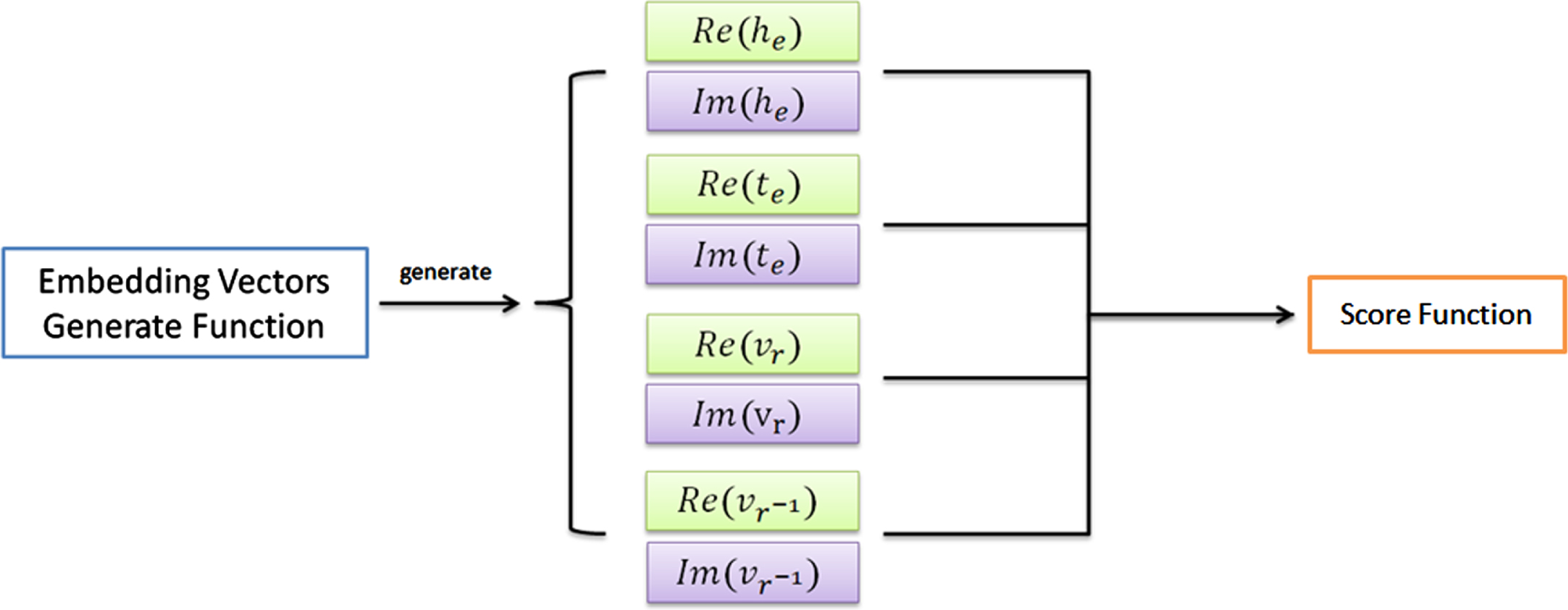
Embedding vectors after mapping into complex space, where Re(x) represents the real part of x, Im(x) represents the imaginary part of x.

3.3 Score function in complex space

In SimplE, $h_{e}, t_{e} \in ℝ^{d}$ are the embedding vectors for an entity e and $v_{r}, v_{r^{- 1}} \in ℝ^{d}$ are the embedding vectors for a relation r. For a triple (e_i, r, e_j), the score function in SimplE is $\frac{1}{2} (〈 h_{e_{i}}, v_{r}, t_{e_{j}} 〉 + 〈 h_{e_{j}}, v_{r^{- 1}}, t_{e_{i}} 〉)$ . Based on CompleX, the score function ψ (s, r, o) of a triple (s, r, o) in complex space is

$ψ (s, r, o) = Re (〈 w_{r}, e_{s}, \bar{e_{o}} 〉)$ (1) where 〈 .〉 denotes the generalized dot product. According to the definition of dot product, Equation 1 can be rewritten as

$ψ (s, r, o) = Re (\sum_{i = 1}^{d} w_{ri} e_{si} {\bar{e}}_{oi})$ (2) where $w^{r} \in ℂ^{d}$ is a complex vector. According to the rules of complex number operations, Equation 2 can be rewritten as

$\begin{matrix} ψ (s, r, o) = 〈 Re (w_{r}), Re (e_{s}), Re (e_{o}) 〉 \\ + 〈 Re (w_{r}), Im (e_{s}), Im (e_{o}) 〉 \\ + 〈 Im (w_{r}), Re (e_{s}), Im (e_{o}) 〉 \\ - 〈 Im (w_{r}), Im (e_{s}), Re (e_{o}) 〉 \end{matrix}$ (3) where Re(x) represents the real part of x, Im(x) represents the imaginary part of x, $\bar{.}$ represents the conjugate of the complex vector and $w_{r} \in ℂ^{K}$ is a complex vector.

Therefore, the score function ψ (e_i, r, e_j) in complex space for a triple (e_i, r, e_j) of our method is:

$\begin{matrix} ψ (e_{i}, r, e_{j}) = & \frac{1}{2} (Re (〈 h_{e_{i}}, v_{r}, \bar{t_{e_{j}}} 〉) \\ + Re (〈 h_{e_{j}}, v_{r^{- 1}}, \bar{t_{e_{i}}} 〉)) \end{matrix}$ (4) where h_{e
_j} represents the inverse head entity embedding vector formed by the combination of tail entity e_j and head entity embedding matrix h, t_{e
_i} represents the inverse tail entity embedding vector formed by the combination of head entity e_i and tail entity embedding matrix t, v_{r
^-1} represents the inverse relation embedding vector. According to the definition of dot product, Equation 4 can be rewritten as

$\begin{matrix} ψ (e_{i}, r, e_{j}) = & \frac{1}{2} (Re (\sum_{k = 1}^{K} h_{e_{i} k} v_{rk} \bar{t_{e_{j} k}}) \\ + Re (\sum_{k = 1}^{K} h_{e_{j} k} v_{r^{- 1} k} \bar{t_{e_{i} k}})) . \end{matrix}$ (5)

According to the rules of complex number operations, the final score function is

$\begin{matrix} ψ (e_{i}, r, e_{j}) = & \frac{1}{2} ((\begin{matrix} Re (h_{e_{i}}), Re (v_{r}), Re (t_{e_{j}}) \\ + Re (h_{e_{i}}), Im (v_{r}), Im (t_{e_{j}}) \\ + Im (h_{e_{i}}), Re (v_{r}), Im (t_{e_{j}}) \\ - Im (h_{e_{i}}), Im (v_{r}), Re (t_{e_{j}}) \end{matrix}) \\ + (\begin{matrix} Re (h_{e_{j}}), Re (v_{r^{- 1}}), Re (t_{e_{i}}) \\ + Re (h_{e_{j}}), Im (v_{r^{- 1}}), Im (t_{e_{i}}) \\ + Im (h_{e_{j}}), Re (v_{r^{- 1}}), Im (t_{e_{i}}) \\ - Im (h_{e_{j}}), Im (v_{r^{- 1}}), Re (t_{e_{i}}) \end{matrix})) \end{matrix}$ (6)

3.4 Model learning

Compared with batch gradient descent (BGD) using all data to calculate the gradient at once, stochastic gradient descent (SGD) updates the gradient for each sample every time it is updated. In our method, we use SGD with mini-batch for learning. Complex-InversE select n triples from the dataset as the positive batch then use the positive batch to generate negative batch by corrupting positive triples.

Figure 4 shows the process of corrupting a triple in Complex-InversE. For a positive triple (h, r, t), we randomly choose the head or tail to corrupt. If the head is chosen, we replace h with ɛ -{ h } where ɛ represents the collection of all entities. If the tail is chosen, we replace t with ɛ -{ t }. We define the label l, for positive triples, l is set to+1 and for negative triples, l is set to -1. Based on Trouillon and Nickel [19], Complex-InversE uses log-likelihood loss function to alleviate overfitting problem. This method choose the L2 regularized negative log-likelihood to optimize:

$\begin{matrix} Loss = & \sum_{((h, r, t), l) \in LB} softplus (- l \cdot φ (h, r, t)) \\ + λ {∥ θ ∥}_{2}^{2}, \end{matrix}$ (7) where θ represents the parameters in the embeddings, l represents the label of a triple, LB represents the batch of labels of triples, φ (h, r, t) represents the score of a triple (h, r, t), λ is the regularization hyperparameter, and softplus(x)=log(1 + exp(x)).

Fig. 4

The process of corrupting a triple, where ɛ represents the collection of all entities.

3.5 Dropout

Based on Hinton and Srivastava [20], we know that dropout can effectively alleviate overfitting and achieve regularization to a certain extent. The idea of dropout can be summarized as letting the activation value of a neuron stop working with a certain probability p during the process of forward propagation in order to make the model more general. When dot products are used to deal with the antisymmetric relationship, the parameter space of the model will inevitably expand and implied an explosion of the number of parameters, making models prone to overfifitting. Complex-InversE aims to improve the accuracy of link predictions by alleviating the overfitting that occurs when dealing with antisymmetric relations. Meanwhile, Dropout can also handle the problem of overfitting and enhance the effect of the model.

Algorithm 1 shows the process of Dropout in Complex-InversE.

Algorithm 1 The process of dropout
1: Input embedding vectors $h_{e}, t_{e}, v_{r}, v_{r^{- 1}} \in ℂ^{d}$ to the neural network as input neuron
2: Randomly remove half of the hidden neurons in the neural network
3: Perform the process of forward propagation on the modified neural network then backpropagate the loss
4: for iteration = 1,2, ... do
5: Restore the removed neurons
6: Randomly select a half-sized subset from the neurons of hidden layer to temporarily remove and back up the parameters of the removed neurons
7: Perform the process of forward propagation then backpropagate the loss. At this moment, the parameters of the neurons that have not been removed are updated, and the parameters of the removed neurons remain unchanged
8: end for
9: The trained vectors $h_{e}, t_{e}, v_{r}, v_{r^{- 1}} \in ℂ^{d}$ is output as output neurons

3.6 Early stopping

Early stopping method is a widely used method, which performs better than the regularization method in many cases. By calculating the performance of the model on the valid dataset during training, we can stop training when the model’s performance on the valid dataset begins to decline in order to avoid overfitting due to continued training.

Algorithm 2 shows the process of Early-Stopping in Complex-InversE.

Algorithm 2 The process of Early-Stopping
1: Divide the dataset into training set, validation set and test set
2: fort = 1,2, ... T do
3: Perform the i-th iteration training on the training set
4: if t% n==0
5: Save the current parameters par_tn
6: end for
7: forv = n, 2n, ... , tn do
8: Use the parameters par_v to perform link prediction on the validation set and save the result accuracy R_v
8: ifR_v > R_v-1 (R₀ = 0)
9: par_best = par_v
10: end for
11: Use the parameters par_best to perform link prediction on the test set and save the final result accuracy R_best

3.7 Time and space complexity analysis

This section compares the scoring function, time complexity and space complexity of Complex-InversE with other link prediction methods. Complex-InversE improves the accuracy of the model while restricting the time complexity and space complexity within a reasonable range. The details are shown in Table 1.

Table 1
Scoring functions of state-of-the-art link prediction models, the dimensionality of their relation parameters, and significant terms of their time and space complexity. d_e and d_r are the dimensionalities of entity and relation embeddings, while n_e and n_r denote the number of entities and relations respectively. $h_{e_{s}}, t_{e_{s}} \in ℝ^{d_{e}}$ are the head and tail entity embedding of entity e_s, and $w_{r^{- 1}} \in ℝ^{d_{r}}$ is the embedding of relation r^-1 (which is the inverse of relation r). 〈 . 〉 denotes the generalized dot product, $\bar{.}$ denotes conjugate of complex vectors and ★ denotes the circular correlation operation

Model Scoring function Relation parameters Space complexity Time complexity

RESCAL (Nickel et al., 2011) $e_{s}^{T} W_{r} e_{o}$ $W_{r} \in ℝ^{d_{e}^{2}}$ $O (n_{e} d_{e} + n_{r} d_{r}^{2})$ $O (d_{e}^{2})$

DistMult (Yang et al., 2015) 〈e_s, w_r, e_o〉 $w_{r} \in ℝ^{d_{e}}$ $O (n_{e} d_{e} + n_{r} d_{e})$ $O (d_{e})$

ComplEx (Trouillon et al., 2016) $Re (〈 e_{s}, w_{r}, \bar{e_{o}} 〉)$ $w_{r} \in ℂ^{d_{e}}$ $O (n_{e} d_{e} + n_{r} d_{e})$ $O (d_{e})$

HolE (Nickel et al., 2016b) 〈w_r, e_s★ e_o 〉 $w_{r} \in ℝ^{d_{e}}$ $O (n_{e} d_{e} + n_{r} d_{e})$ $O (d_{e} log d_{e})$

SimplE (Kazemi and Poole, 2018) $\frac{1}{2} (〈 h_{e_{s}}, w_{r}, h_{e_{o}} 〉 + 〈 h_{e_{o}}, w_{r^{- 1}}, h_{e_{s}} 〉)$ $w_{r} \in ℝ^{d_{e}}$ $O (n_{e} d_{e} + n_{r} d_{e})$ $O (d_{e})$

Complex-InversE (ours) $\frac{1}{2} (Re (〈 h_{e_{s}}, w_{r}, h_{e_{o}} 〉) + Re (〈 h_{e_{o}}, w_{r^{- 1}}, h_{e_{s}} 〉))$ $w_{r} \in ℂ^{d_{e}}$ $O (n_{e} d_{e} + n_{r} d_{e})$ $O (d_{e})$

Model	Scoring function	Relation parameters	Space complexity	Time complexity
RESCAL (Nickel et al., 2011)	$e_{s}^{T} W_{r} e_{o}$	$W_{r} \in ℝ^{d_{e}^{2}}$	$O (n_{e} d_{e} + n_{r} d_{r}^{2})$	$O (d_{e}^{2})$
DistMult (Yang et al., 2015)	〈e_s, w_r, e_o〉	$w_{r} \in ℝ^{d_{e}}$	$O (n_{e} d_{e} + n_{r} d_{e})$	$O (d_{e})$
ComplEx (Trouillon et al., 2016)	$Re (〈 e_{s}, w_{r}, \bar{e_{o}} 〉)$	$w_{r} \in ℂ^{d_{e}}$	$O (n_{e} d_{e} + n_{r} d_{e})$	$O (d_{e})$
HolE (Nickel et al., 2016b)	〈w_r, e_s★ e_o 〉	$w_{r} \in ℝ^{d_{e}}$	$O (n_{e} d_{e} + n_{r} d_{e})$	$O (d_{e} log d_{e})$
SimplE (Kazemi and Poole, 2018)	$\frac{1}{2} (〈 h_{e_{s}}, w_{r}, h_{e_{o}} 〉 + 〈 h_{e_{o}}, w_{r^{- 1}}, h_{e_{s}} 〉)$	$w_{r} \in ℝ^{d_{e}}$	$O (n_{e} d_{e} + n_{r} d_{e})$	$O (d_{e})$
Complex-InversE (ours)	$\frac{1}{2} (Re (〈 h_{e_{s}}, w_{r}, h_{e_{o}} 〉) + Re (〈 h_{e_{o}}, w_{r^{- 1}}, h_{e_{s}} 〉))$	$w_{r} \in ℂ^{d_{e}}$	$O (n_{e} d_{e} + n_{r} d_{e})$	$O (d_{e})$

4 Experiments and results

4.1 Datasets

We conducted experiments on four widely used datasets. The overview of our datasets is in Table 2.

Table 2
The overview of used datasets which include the number of entities and relations

Datasets #entity #relation #training #validation #test

FB15k 14,951 1,345 483,142 50,000 59,071

WN18 40,943 18 141,442 5,000 5,000

FB15k-237 14,541 237 272,115 17,535 20,466

WN18RR 40,943 11 86,835 3,034 3,134

Datasets	#entity	#relation	#training	#validation	#test
FB15k	14,951	1,345	483,142	50,000	59,071
WN18	40,943	18	141,442	5,000	5,000
FB15k-237	14,541	237	272,115	17,535	20,466
WN18RR	40,943	11	86,835	3,034	3,134

FB15K: FB15k is a series of triples extracted from Freebase [4]. The main relation patterns in FB15K are symmetry/antisymmetry and inversion.

FB15K-237 [21]: FB15K-237 is a subset of FB15k, where inverse relations are deleted. The main relation patterns in FB15K-237 are symmetry/antisymmetry and composition.

WN18[11]: WN18 is a subset of WordNet [6], its entities (termed synsets) correspond to senses, and relation types define lexical relations between those senses. The main relation patterns in WN18 are symmetry/antisymmetry and inversion.

WN18RR [16]: WN18RR is a subset of WN18, where inverse relations are deleted. The main relation patterns are symmetry/antisymmetry and composition.

4.2 Evaluation metrics

Based on [11], Complex-InversE use the filtered setting. While evaluating on test triples, we filter out all the valid triples from the candidate set, which is generated by either corrupting the head or tail entity of a triple. Complex-InversE use two classic evaluation indicators to judge the performance of our model on the data set: Mean Reciprocal Rank (MRR) and Hits@k. The key idea of MRR is that the quality of the result depends on the position of the first correct answer, which means that the higher the first correct answer, the better the result. The key idea of HIT@k is that the quality of the result depends on whether there exists a real entity in the top k of the predicted result.

4.3 Baselines

In our experiments, we compared our model with several baselines, which can be divided into Neural and Non-neural. Neural represents methods that involve neural networks in the modeling process, like ConvE [13] and R-GCN [22]. Non-neural represents methods that do not involve neural networks in the modeling process, like DistMult [14], ComplEx [19] and SimplE [10].

4.4 Implementation

We fixed the maximum number of iterations to 1500 and the batch size to 100 on Complex-InversE. We set the learning rate for WN18 and WN18RR to 0.1 and for FB15k and FB15k-237 to 0.05 and used adagrad to update the learning rate after each batch. Based on our research in Section 4.7 and 4.8, we set the dropout rate to 0.2 and generated one negative example per positive example for WN18 and WN18RR and 25 negative examples per positive example in FB15k and FB15k-237. We computed the filtered MRR of our model over the validation set every 50 iterations for WN18 and WN18RR and every 100 iterations for FB15k and FB15k-237 and selected the iteration that resulted in the best validation filtered MRR. The best embedding size and λ values for WN18 and WN18RR were 200 and 0.03, for FB15k and FB15k-237 were 200 and 0.1.

4.5 Results

Figure 5 Accuracy comparison between other benchmark methods and Complex-InversE, where a positive value indicates that the accuracy of Complex-InversE in this evaluation metric is higher than this model, and a negative value indicates that the accuracy of Complex-InversE in this evaluation index is lower than this model. All accuracy comparisons are expressed as percentages.

Fig. 5

(a) Accuracy comparison between other benchmark methods and Complex-InversE on FB15K.

Fig. 5

(b) Accuracy comparison between other benchmark methods and Complex-InversE on WN18.

Fig. 5

(d) Accuracy comparison between other benchmark methods and Complex-InversE on WN18RR.

We compare the results of Complex-InversE with other baseline methods to prove the effectiveness of Complex-InversE. The results on the four link prediction datasets are summarized in Table 3 and Table 4. Figure 5 shows the accuracy comparison between other benchmark methods and Complex-InversE in percentage terms. We can see that Complex-InversE achieved better results on the three datasets compared to the existing baselines in the same datasets.

Table 3

Results on WN18 and FB15k. Best results are in bold

	FB15K				WN18
	MRR	Hit@1	Hit@3	Hit@10	MRR	Hit@1	Hit@3	Hit@10
TransE (Bordes et al., 2013)	0.380	0.231	0.472	0.641	0.454	0.089	0.823	0.934
HolE (Trouillon et al., 2017)	0.524	0.402	0.613	0.739	0.938	0.930	0.945	0.949
DistMult (Yang et al., 2015)	0.654	0.546	0.733	0.824	0.822	0.728	0.914	0.936
ComplEx (Trouillon et al., 2016)	0.692	0.599	0.759	0.840	0.941	0.936	0.936	0.947
SimplE (Kazemi et al., 2018)	0.727	0.660	0.773	0.838	0.942	0.939	0.944	0.947
R-GCN (Schlichtkrull et al., 2018)	0.696	0.601	0.760	0.842	0.819	0.697	0.929	0.964
ConvE (Dettmers et al., 2018)	0.657	0.558	0.723	0.831	0.943	0.935	0.946	0.956
D4-Gumbel (Xu et al., 2019)	0.728	0.648	0.782	0.864	0.946	0.942	0.948	0.952
InteractE (Vashishth et al., 2020)	0.527	0.415	0.594	0.723	0.941	0.930	0.95	0.956
CrossE (Zhang et al., 2019)	0.728	0.634	0.802	–	0.830	0.741	0.931	–
Complex-InversE	0.770	0.714	0.804	0.871	0.947	0.942	0.951	0.956

Table 4

Results on WN18RR and FB15k-237. Best results are in bold

	FB15K-237				WN18RR
	MRR	Hit@1	Hit@3	Hit@10	MRR	Hit@1	Hit@3	Hit@10
DistMult(Yang et al., 2015)	0.240	0.155	0.263	0.419	0.430	0.390	0.440	0.490
ComplEx (Trouillon et al., 2016)	0.247	0.158	0.275	0.428	0.440	0.410	0.460	0.510
SimplE(Kazemi et al., 2018)	0.165	0.089	0.176	0.327	0.394	0.381	0.400	0.416
R-GCN(Schlichtkrull et al., 2018)	0.248	0.151	0.264	0.417	–	–	–	–
RotatE(Sun et al., 2019)	0.297	0.205	0.328	0.48	0.476	0.428	0.492	0.571
D4-Gumbel(Xu et al., 2019)	0.300	0.204	0.332	0.496	0.442	0.505	0.557	0.486
MINERVA (Das et al., 2018)	0.293	0.217	0.329	0.456	–	–	–	–
CrossE(Zhang et al., 2019)	0.299	0.211	0.331	0.474	–	–	–	–
Complex-InversE	0.309	0.221	0.341	0.487	0.433	0.392	0.451	0.527

On FB15K, Complex-InversE outperforms the baseline methods on four evaluation metrics.On WN18, Complex-InversE outperforms the baseline methods on three evaluation metrics, but the increase of accuracy compared to the original model is not significant. We believe that since the main relation patterns in FB15K and WN18 are symmetry/antisymmetry and inversion, and the model of entities and relations in complex space can effectively handle antisymmetric relations, Complex-InversE performs satisfactorily on FB15K and WN18. For most triples in FB15K, the types of head and tail entities are different, while almost all entities in WN18 are words and belong to the same entity type. Since Complex-InversE can deal with the problem of a small number of relations and entities to effectively improve model performance, we believe that this is the key for Complex-InversE to effectively deal with the problem of more triple types and less number of each type in FB15K to improve the model performance.

For the same reason, Complex-InversE performs better on FB15K-237 than on WN18RR. On FB15K-237, Complex-InversE performed satisfactorily, while on WN18RR, Complex-InversE performed worse than baseline methods. Complex-InversE significantly improves the accuracy of the original model SimplE on both FB15K-237 and WN18RR. Since the main relation pattern in FB15K-237 and WN18RR is composition and the original model SimplE is not good at handling the composition relation pattern, the results on FB15K-237 and WN18RR are worse than on FB15K and WN18, although the accuracy has been significantly improved compared to the original model SimplE. Specially, since WN18RR has both two unfavorable factors for Complex-InversE, i.e. the single entity type with large quantity and containing composition relation pattern, Complex-InversE performed worse than baseline methods on WN18RR.

4.6 Ablation experiment

In this section, we conduct ablation experiments on Complex-InversE to prove that our ideas are indeed effective. The experimental results are shown in Table 5.

Table 5
Ablation experiment on FB15K

MRR Hit@1 Hit@3 Hit@10

SimplE 0.727 0.660 0.773 0.838

SimplE+complex vectors 0.740 0.676 0.783 0.851

SimplE+Dropout 0.749 0.675 0.804 0.871

Complex-InversE – complex vectors 0.754 0.681 0.813 0.880

Complex-InversE – Dropout 0.751 0.683 0.792 0.861

Complex-InversE – Early-Stopping 0.765 0.708 0.799 0.865

Complex-InversE 0.770 0.714 0.804 0.871

	MRR	Hit@1	Hit@3	Hit@10
SimplE	0.727	0.660	0.773	0.838
SimplE+complex vectors	0.740	0.676	0.783	0.851
SimplE+Dropout	0.749	0.675	0.804	0.871
Complex-InversE – complex vectors	0.754	0.681	0.813	0.880
Complex-InversE – Dropout	0.751	0.683	0.792	0.861
Complex-InversE – Early-Stopping	0.765	0.708	0.799	0.865
Complex-InversE	0.770	0.714	0.804	0.871

From Table 5, we can see that the complex vector embedding, Dropout, and Early-Stopping all contribute to the accuracy improvement of the original model SimplE. At the same time, the lack of any improvement will reduce the performance of Complex-InversE, which proves that every improvement is effective. Complex vectors can effectively capture antisymmetric relations, Dropout and Early-Stopping can deal with the problem of a small number of relations and entities to alleviate overfitting.

4.7 Influence of dropout rate

We investigated the influence of dropout rate in the process of Dropout. Dropout rate represents the proportion of neurons temporarily deleted during the process of Dropout. For example, if dropout rate = 0.5, half of the neurons will be temporarily deleted during the process of Dropout. We focused on FB15K and let dropout rate vary in {0.1, 0.2, 0.3, 0.4, 0.5}.

Figure 6 shows the effect of dropout rate on the performance of Complex-InversE on FB15K. If the dropout rate is too large, too many neurons are temporarily deleted during training, and the model changes from overfitting to underfitting, which reduces the accuracy of the model. If dropout rate is too small, too few neurons are temporarily deleted during training, which cannot effectively alleviate overfitting. When dropout rate = 0.2, MRR and Hit@1 reach the highest value. When dropout rate = 0.3, Hit@3 and Hit@10 reach the highest value. Since MRR and Hit@1 can better show the accuracy of a link prediction method, we set the best dropout rate to 0.2.

Fig. 6

Influence of dropout rate on the filtered test MRR. The number of negative triples generated per positive training example is 10.

4.8 Influence of negative samples

We further investigated the influence of the number of negatives generated per positive training sample. We focused on FB15K, with the best hyper-parameters, obtained from the previous experiment. We then let η vary in {1, 5, 10, 15, 20, 25}.

Figure 7 shows the influence of the number of generated negatives per positive training triple on the performance of our model on FB15K. Generating more negatives clearly improves the results, but also increases training time. We choose 20 negatives a good trade-off between accuracy and training time.

Fig. 7

Influence of the number of negative triples generated per positive training example on the filtered test MRR and on training time to convergence on FB15K for Complex-InversE.

5 Conclusion

This paper proposes Complex-InversE, a knowledge graph link prediction method in complex space. Complex-InversE uses three key ideas to improve the model performance, complex embedding vectors, Dropout, and Early-Stopping. Through experiments, we demonstrate that Complex-InversE achieves a consistent improvement on link prediction performance on multiple datasets. We also theoretically analyze the effectiveness of the components of Complex-InversE, and provide empirical validation of our hypothesis that mapping embedding vectors to complex space is beneficial for link prediction on bilinear models.

References

Zhang

, Yuan

N.J.

, Lian

, Xie

and Ma

W.-Y.

, Collaborative knowledge base embedding for recommender systems, In Proceedings of the 22nd International Conference on Knowledge Discovery and Data Mining, KDD ’16 (2016), 353–362.

Xiong

, Power

and Callan

, Explicit semantic ranking for academic search via knowledge graph embedding, In Proceedings of the 26th International Conference on World Wide Web, pp. 1271–1279. International World Wide Web Conferences Steering Committee, 2017.

Yang

and Mitchell

, Leveraging knowledge bases in lstms for improving machine reading, In Proceedings of the 55th Annual Meeting of the Association for Computational Linguistics (Volume 1: Long Papers), volume 1 (2017), pp. 1436–1446.

Bollacker

, Evans

, Paritosh

, Sturge

and Taylor

, Freebase: A collaboratively created graph database for structuring human knowledge, In Proceedings of the 2008 ACM SIGMOD International Conference on Management of Data, SIGMOD ’08, 1247–1250. New York, NY, USA: ACM, 2008.

Suchanek

F.M.

, Kasneci

and Weikum

, Yago: A Core of Semantic Knowledge, In 16th International Conference on the World Wide Web (2007), 697–706.

Miller

G.A.

, WordNet: a lexical database for English[J], Communications of the Acm 38(11) (1995), 39–41.

Sun

, Deng

Z.-H.

and Nie

J.-Y.

, RotatE Knowledge Graph Embedding by Relational Rotation in Complex, In ICLR, 2019.

Vashishth

, Sanyal

, Nitin

, et al., InteractE: Improving Convolution-Based Knowledge Graph Embeddings by Increasing Feature Interactions[J], Proceedings of the AAAI Conference on Artificial Intelligence 34(3) (2020), 3009–3016.

Zhang

, Tay

, Yao

and Liu

, Quaternion Knowledge Graph Embeddings, In NeurIPS, 2019.

10.

Kazemi

S.M.

and Poole

, Simple embedding for link prediction in knowledge graphs, In NeurIPS (2018c).

11.

Bordes

, Usunier

, Garcia-Duran

, Weston

and Yakhnenko

, Translating embeddings for modeling multi-relational data, In Advances in Neural Information Processing Systems (2013), 2787–2795.

12.

Wang

, Zhang

, Feng

, et al., Knowledge Graph Embedding by Translating on Hyperplanes[C], AAAI 14 (2014), 1112–1119.

13.

Lin

, Liu

, Sun

, Liu

and Zhu

, Learning Entity and Relation Embeddings for Knowledge Graph Completion, In AAAI, 2015.

14.

Yang

, Yih

, He

, Gao

and Deng

, Embedding entities and relations for learning and inference in knowledge bases, CoRR abs/1412.6575, 2014.

15.

Trouillon

, Welbl

, Riedel

, Gaussier

and Bouchard

, Complex embeddings for simple linkprediction, In ICML (2016), 2071–2080.

16.

Nickel

, Tresp

and Kriegel

H.-P.

, A three-way model for collective learning on multi-relational data, In ICML, volume 11 (2011), pages 809–816.

17.

Dettmers

, Minervini

, Stenetorp

and Riedel

, Convolutional 2d knowledge graph embeddings, In Thirty-Second AAAI Conference on Artificial Intelligence, 2018.

18.

Nguyen

D.Q.

, Nguyen

T.D.

, Nguyen

D.Q.

and Phung

, A novel embedding model for knowledge base completion based on convolutional neural network, In Proceedings of North American Chapter of the Association for Computational Linguistics (2018), 327–333.

19.

Nguyen

D.Q.

, Vu

, Nguyen

T.D.

, et al., A Capsule Network-based Embedding Model for Knowledge Graph Completion and Search Personalization[C], Proceedings of the 2019 Conference of the North, 2019.

20.

Hinton

G.E.

, Srivastava

, Krizhevsky

, et al., Improving neural networks by preventing co-adaptation of feature detectors[J], Computer ENCE 3(4) (2012), 212–223.

21.

Toutanova

and Chen

, Observed versus latent features for knowledge base and text inference, In Proceedings of the 3rd Workshop on Continuous Vector Space Models and their Compositionality, 2015, pp. 57–66.

22.

Schlichtkrull

, Kipf

T.N.

, Bloem

, Berg

R.v.d.

, Titov

and Welling

, Modeling relational data with graph convolutional networks, arXiv preprint arXiv:1703.06103, 2017.

Complex-InversE: Improving bilinear knowledge graph embeddings by mapping into complex space

Abstract

1 Introduction

2 Related work

3 Complex-InversE

3.1 Model framework

3.6 Early stopping

3.7 Time and space complexity analysis

4.1 Datasets

Table 2 The overview of used datasets which include the number of entities and relations Datasets #entity #relation #training #validation #test FB15k 14,951 1,345 483,142 50,000 59,071 WN18 40,943 18 141,442 5,000 5,000 FB15k-237 14,541 237 272,115 17,535 20,466 WN18RR 40,943 11 86,835 3,034 3,134

4.3 Baselines

4.4 Implementation

4.5 Results

References