A new approach for data augmentation in a deep neural network to implement a monitoring system for detecting prostate cancer in MRI images 1

Abstract

Prostate cancer is one of the most common cancers in men, which takes many victims every year due to its latent symptoms. Thus, early diagnosis of the extent of the lesion can help the physician and the patient in the treatment process. Nowadays, detection and labeling of objects in medical images has become especially important. In this article, the prostate gland is first detected in T2 W MRI images by the Faster R-CNN network based on the AlexNet architecture and separated from the rest of the image. Using the Faster R-CNN network in the separation phase, the accuracy will increase as this network is a model of CNN-based target detection networks and is functionally coordinated with the subsequent CNN network. Meanwhile, the problem of insufficient data with the data augmentation method was corrected in the preprocessing stage, for which different filters were used. Use of different filters to increase the data instead of the usual augmentation methods would eliminate the preprocessing stage. Also, with the presence of raw images in the next steps, it was proven that there was no need for a preprocessing step and the main images could also be the input data. By eliminating the preprocessing step, the response speed increased. Then, in order to classify benign and malignant cancer images, two deep learning architectures were used under the supervision of ResNet18 and GoogleNet. Then, by calculating the Confusion Matrix parameters and drawing the ROC diagram, the capability of this process was measured. By obtaining Accuracy = 95.7%, DSC = 96.77% and AUC = 99.17%, The results revealed that this method could outperform other well-known methods in this field (DSC = 95%) and (AUC = 91%).

Keywords

Prostate cancer data augmentation filtering feature extraction localization deep learning

Abbreviations

Acronyms

DRE

Digital Rectal Exam

PSA

prostate-specific Antigen

PI-RADS

Prostate Imaging Reporting & Data System

MRI

Magnetic resonance imaging

CNN

convolutional neural network

R-CNN

Region convolutional neural network

SVM

support vector machine

Gleason score

ROC

Receiver operating characteristic

DSC

Dice similarity coefficient

AUC

Area under the curve

transition zone

DCE

Dynamic Contrast-Enhanced

peripheral zone

RPN

Region proposal network

1 Introduction

Prostate cancer is common in men with 85% of men aged 65 and over suffering this disease. It kills about 250,000 people every year, and may not show symptoms until advanced stage; as such mortality from it is more common than other types of cancer [1, 2].

The causes of prostate cancer are different, including risk factors such as age, ethnicity, genetic factors, and family background [3]. Environmental factors also affect the disease development, including poor nutrition such as consumption of red meat, low consumption of fruits, vegetables, and vitamins, obesity and physical inactivity, plus high blood glucose levels [4].

There are many ways to diagnose prostate cancer where a doctor may use one or more tests for the diagnosis including DRE, biopsy, and PSA as the most important indicators of prostate cancer screening [5, 6].

Diagnosis of prostate cancer and its proper staging play essential roles in its clinical care; hence, magnetic resonance imaging for the localization and disease progression has become necessary for physicians in recent decades to improve the correct clinical diagnosis. As this disease is very heterogeneous, the combined use of these tools helps physicians and patients choose the most appropriate treatment.

Magnetic resonance imaging (MRI) is an advanced medical imaging technique used to produce quality images of different parts of the human body. MRI is indeed a method that uses magnetic properties of tissues and generates images. In the MRI pictures of prostate, the images consist of details that indicate the morphological and functional responses of the prostate gland [7]. Regarding the basic principles of MRI, the nuclei of some elements will be aligned with the magnetic force when placed in a strong magnetic field, where the signal strength in the MRI occurs due to two factors, proton density and relaxation times T1 and T2.

T1 is a time when 63% of the longitudinal magnetic moment of a proton returns from the direction perpendicular to the field back to the direction parallel to the magnetic field after excitation. T2 is a time when the transverse magnetic moment of a proton decreases to 37% of its original value after excitation. Most pathological processes increase the relaxation times T1 and T2. Thus, the signal will be lower (darker color) in the T1-weighted images and brighter in the T2-weighted images compared to the surrounding natural tissues; hence, the tumors usually have a lower signal strength in MRI with T2-weighted forms [8, 9]. MR image of prostate consists of two major zones, the transition zone (TZ) and peripheral zone (PZ). The T2-weighted method is applicable in the diagnosis of cancers such as prostate cancer to visualize the prostate gland structure and surrounding structures [10]. About 70% of tumors and lesions are in the lateral zone and are easily distinguishable from the prostate gland tissue, but tumors in the central gland may not be distinguishable from the surrounding tissues; hence, it is necessary to provide a good solution for image segmentation.

PI-RADS evaluation classification was based on multipolar MRI findings which is a combination of T2-w and DWI plus Dynamic Contrast-Enhanced Imaging (DCE). PI-RADS evaluation classification determines the clinical risk of cancer [11].

The following images specify the method of classification based on PI-RADS; the transition and peripheral zone classification are shown in Figs. 1 and 2, In Figs. 1 and 2, the exact location of the lesion is indicated by a yellow arrow, As below:

Fig. 1

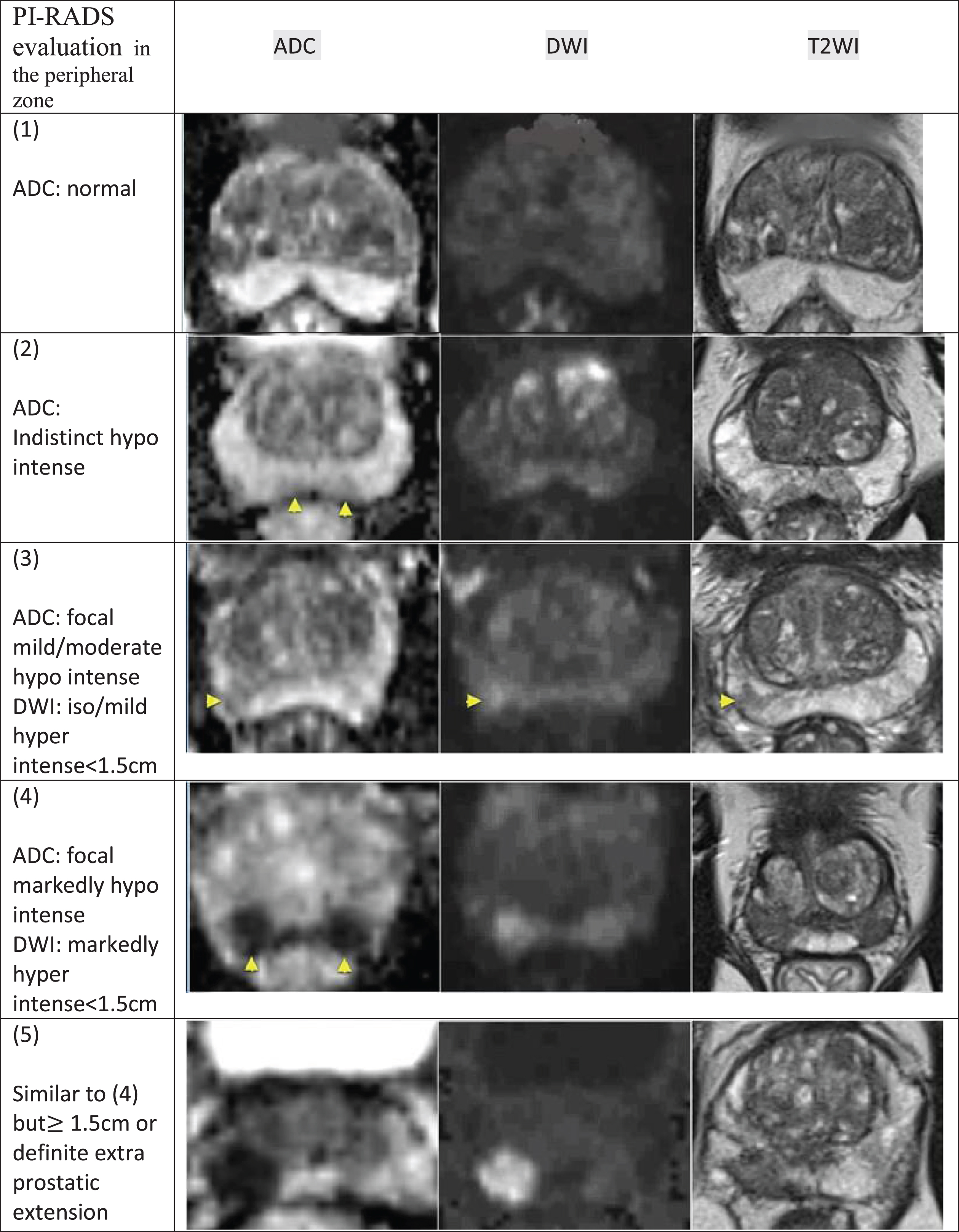
PI-RADS in the peripheral zone. In this figure, prostate cancer is classified in the peripheral area based on the PI-RADS classification.

Fig. 2

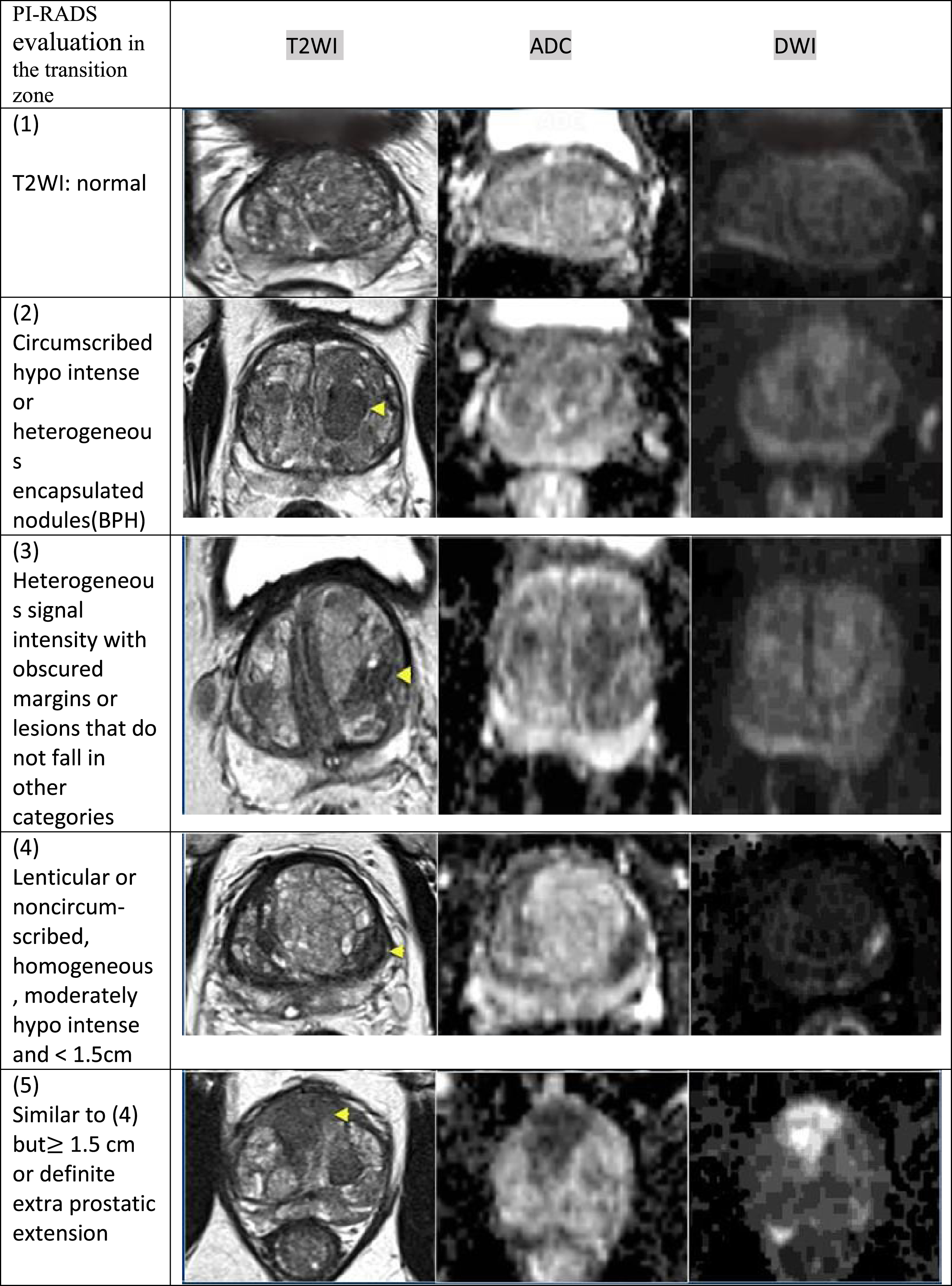
PI-RADS in the transition zone. In this figure, prostate cancer is classified in the transition area based on the PI-RADS classification.

Examples of diagnosing the type of cancer (benign or malignant) are shown in Fig. 3 as follows:

Fig. 3

a) The exact location of the lesion in malignant prostate cancer is marked with a white arrow, b) The exact location of the lesion in Benign prostate cancer is marked with a yellow arrow.

In Fig. 3, the exact location of the lesion is indicated by a white arrow in Malignant prostate cancer and a yellow arrow in Benign prostate cancer.

Thus, the prostate gland must first be separated from the rest of the image; Faster R-CNN has been used based on previous time-consuming methods [12]. Faster R-CNN coordinates the proposed area extraction with CNN; in addition to performing all non-repetitive calculations, it greatly enhances the accuracy of the model. In this network, the features of each convolution layer in the network can be used to predict the proposals of the respective region. Thus, there is no need for an algorithm such as selective search.

The need for large amounts of educational data is an important problem for training the use of deep learning networks. Due to the lack of reliable data, a method called data enhancement should be used in such a set. In the present study, the data enhancement step was performed along with preprocessing.

In the past, many effective studies were conducted to extract features from MRI. For example, in a study, different articles diagnosing prostate cancer were extracted by extracting different features from different images and classifications, and the results were categorized [12, 13]. For instance, in a study by [14], R-CNN was used faster in isolating the prostate gland from other regions using the ResNet101 architecture and was able to get DSC equal to 0.86, while in another article [15], AUC = 0.74. In addition, the diagnosis of benign and malignant cancers was made.

For comparison, in the Results and Discussion section, Tables 3 and 4 report the recent results while Tables 1 and 2 present the results obtained from the proposed method.

2 Material and methods

The present study aimed to improve the accuracy of output calculations while also reducing the computational cost by combining the steps of working with each other. Differentiating the benign from malignant type as well as the use of MRI images with a weight T2 was the distinguishing point of the research. After taking an image from a validated database, as well as data augmentation and its zoning by the Faster R-CNN method, in this study, feature extraction and selection were performed by various CNNs such as GoogleNet, ResNet18, and classified into two types, benign and malignant. The results confirmed the efficiency of the method. Figure 4 displays the block diagram of the proposed method; The work algorithm is also plotted in Fig. 5.

Fig. 4

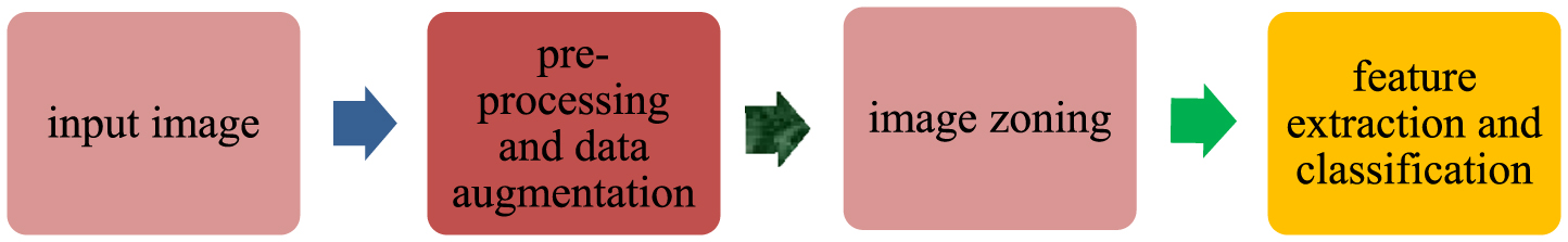
Overview of the proposed method. The MRI image entry stage, the pre-processing and augmentation stage, which are performed simultaneously, the prostate gland separation stage, and finally the feature extraction stage as well as classification of images into two types, benign and malignant.

Fig. 5

The algorithm of the work performed in this research. Faster R-CNN plus CNN function sequences and finally classification of the input image as benign or malignant.

As shown in Fig. 4, in the first step, the MRI images will have a weight of T2, then, we will have the preprocessing and augmentation of the data. In the next step, the prostate area is separated from the background of the image. Finally, by extracting features and classifying, the outputs are separated.

Figure 5 shows the internal function sequence of the Faster R-CNN network as a separator of the prostate gland region from the rest of the image, followed by the extraction of features and classification of images by CNN architectures, and then the separation of images into benign and Malignant will be done.

2.1 Obtaining the image, dataset, classification, and method of its use

The images used came from Harvard University’s Brigham Hospital [16]. In this collection, medical images of 230 patients have been uploaded to the database. There are at least 20 images of each patient with axial, sagittal, and crown protocols for T1 and T2. In addition, there were other pieces of information such as the patient’s age as well as detailed information about the MRI machine. All of the patients listed on this website have had prostate cancer, while whether the disease is benign or malignant has been confirmed by a physician and is included in this study. Note that 11 patients with benign cancer and 20 patients with malignant cancer who were valid in terms of citation were considered, then sent to the next stage using data magnification. Data have been enhanced to increase diagnostic accuracy.

2.2 Preprocessing and data augmentation

Supplying the educational data is a major problem of working with the deep learning networks. Collecting a large number of data is very time consuming and has its own limitations. Sometimes, collecting more data may be unavailable, and training should be done with what is available. The problem will be further complicated since the network is prone to overfitting error and if the data set is not large enough. There is often a method called data augmentation to solve this problem. Data augmentation technique increases educational samples with wider coverage using methods such as rotation, scaling, cutting and transfer, as well as coloring [14, 17]. In this study, instead of using conventional methods due to limitations in the fundamental change of the image, such as rotation, coloring or cutting, the simultaneous processing and improvement of data was used. In other words, the median filters, Gaussian matching, and histogram (optimizing the light intensity of the image) in addition to the original image were considered as images to be trained and tested, so the fact is covered that any image with any noise can be compatible with the system. Figure 6 shows the details of the preprocessing step.

Fig. 6

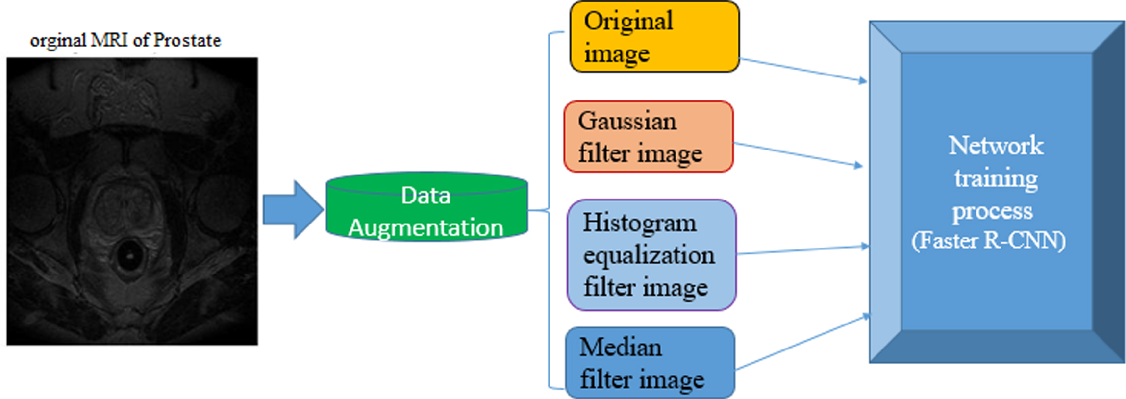
Overview of pre-processing details and data augmentation on the images. Increase the number of images with three different Gaussian, histogram and median filters and have the main images without any pre-processing in the work.

2.2.1 Median filter

Median filter is widely used in image processing. An important feature of this filter, unlike low-pass filters such as medium or box filters, is that it holds the edges in the image. Also, another important feature is that it maintains the position of the edges without shifts [18].

2.2.2 Gaussian filter

Gaussian filter is probably the most useful (but not the fastest) filter. Gaussian filtering is done from the channel of each point in the input array with a Gaussian kernel and then aggregated to obtain the output [19].

2.2.3 Histogram equalization

The histogram matching process is a simple yet efficient technique for increasing image contrast which generally generates satisfactory results. However, due to design limitations, the output images often lose good details or contains unwanted artifacts. One of the reasons for such a defect is the failure of some techniques to make full use of the allowable intensity range in transmitting information taken from an image. The histogram equalization technique will maximize the content of the information within an image [20].

As shown in Fig. 6, in addition to the main images, three types of filters are placed on the images to increase the data. Histogram, Gaussian and Median filters have been selected because of their many image processing properties.

2.3 Zoning

Goal recognition is an important technology in the field of machine vision and image processing. In this regard, the implementation of goal recognition systems in images is an important challenge in many research fields, such as changing viewing angle, background noise, and brightness and Optimization Algorithms [9 , 38–40]. The detection of goals needs presenting the information on the presence of a data class in addition to estimating the spatial coordinates of the target sample(s) in the image. A diagnosis window is considered correct if the detected output zone is reasonably similar to the intended target (usually more than 50%). At this stage, a stage of prostate gland localization was performed by a model of deep learning network, called Faster R-CNN, which had a lower computational load, higher speed, and higher accuracy than previous methods [14].

Faster R-CNN, as a popular zone-based convolution network, significantly reduces training and testing time compared to other convolution networks [21]. Using a deep convolution network compared to other methods, including R-CNN [22], and Fast R-CNN [23], this network does not have repetitive steps and calculations, and is thus a more efficient method than previous methods. Figure 7 depicts how the Faster R-CNN network works.

Fig. 7

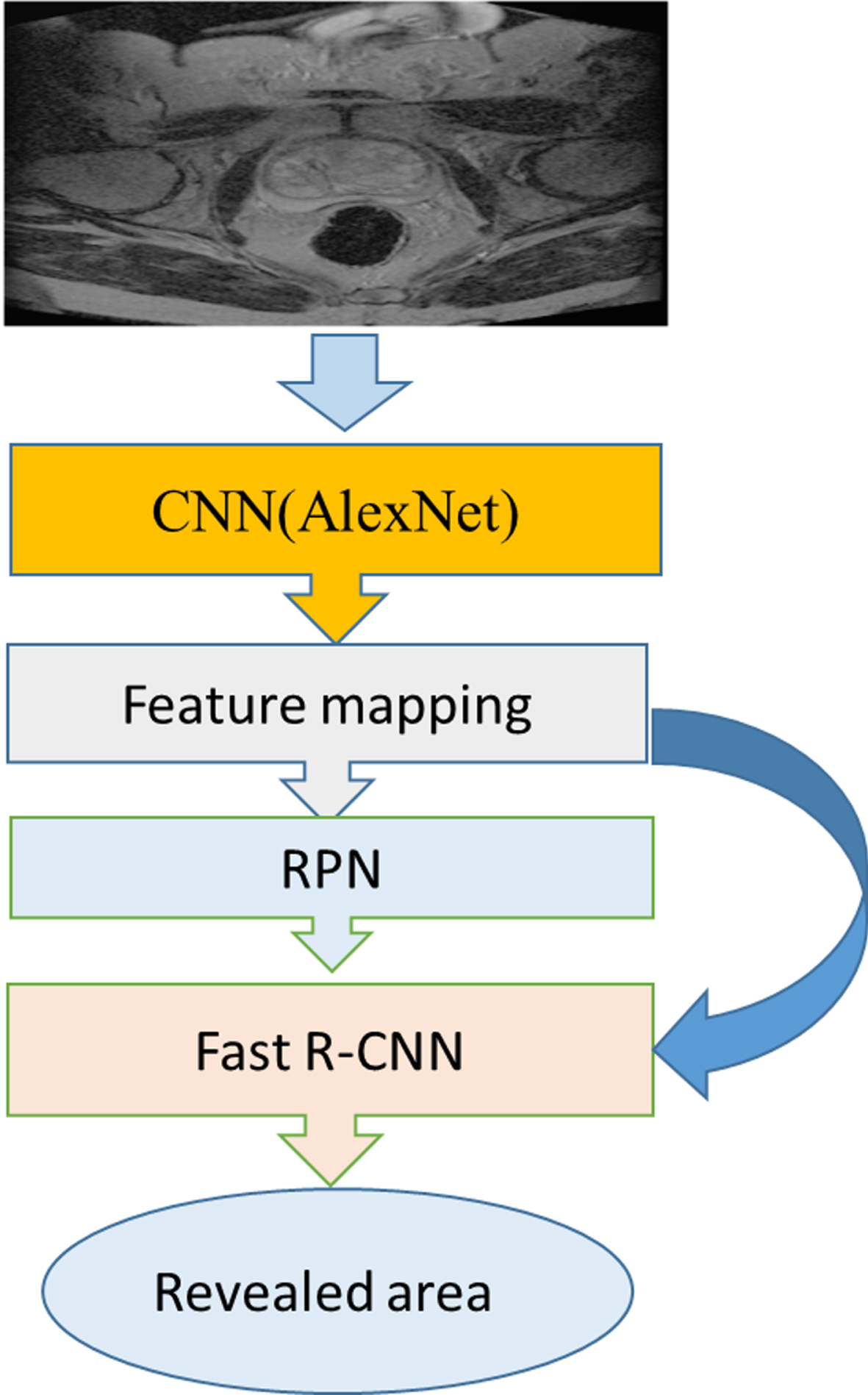
Overview of how the Faster R-CNN network works on the image and extracts the revealed area.

As shown in Fig. 7, an image is first entered as input to the network. This image is given to the selected CNN network to identify important parts, which is called feature mapping, where the image is convoluted in the kernel. The output of the previous network is given to the Region proposal network to specify the proposed components and their rating (RPN). The ROI pooling layer is applied so that all the separated parts are the same size, and finally these equal parts are connected to a fully neural network, which is finally sorted via a softmax layer (Fast R-CNN).

The Faster R-CNN is capable of extracting color information and is a high-level extractor based on the vector dimensions of the higher-level output feature. In this network, two steps are performed. In the first step, it generates a set of proposed zones, and in the second step, it applies a classifier for the classification output of this group of zones. In comparison with one-stage systems such as yolo [24] and SSD [25], this network has advantages such as significantly lower computational costs of the proposed zones. This network has no limit to perform calculations on the size of the input image and can be implemented on real images.

In general, the Faster R-CNN is examined for implementation in MATLAB in three sections, namely data preparation, training, and evaluation. Note that this network is called a ready file in MATLAB. Internal networks, RPN, and Fast R-CNN, existing in this network and internal operations for training are done automatically and without user intervention; however, the training parameters within the network should be selected well and in accordance with the training images to achieve an efficient network. A very strong and well-known architecture, AlexNet [26], was used in the training section. After setting the parameters, the network structure was defined to perform the learning of weights and network bias. Figure 7 demonstrates the function of Faster R-CNN. Figure 8 presents details of selecting the prostate gland by the Faster R-CNN network.

Fig. 8

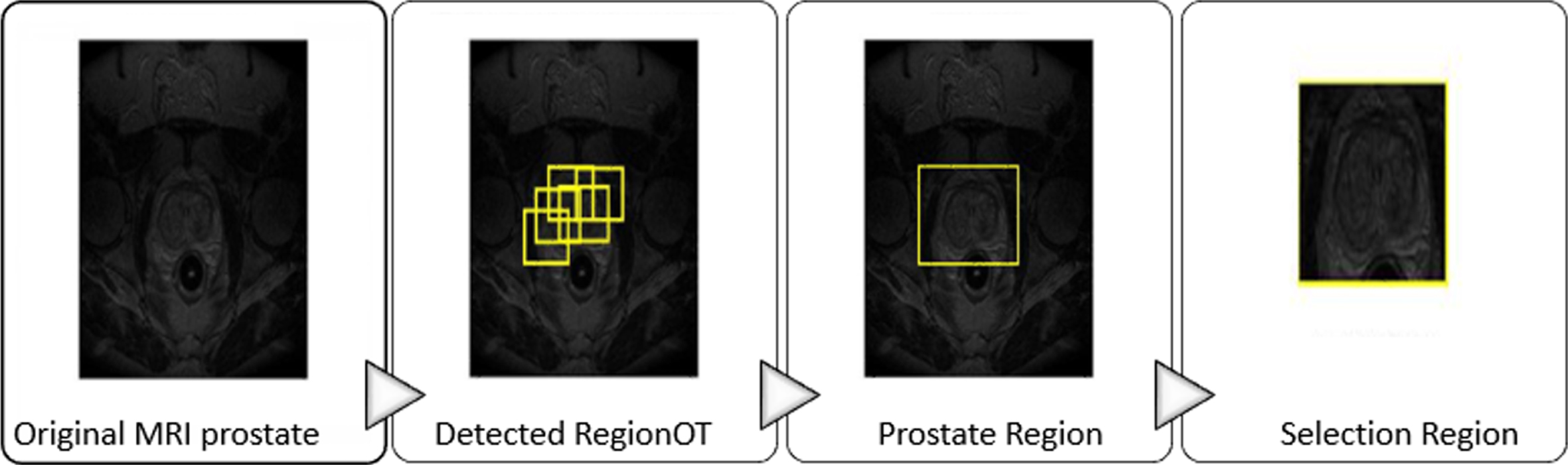
The Faster R-CNN function on the prostate MRI and selection of prostate gland from other zones.

As shown in Fig. 8, the Fast network suggests areas based on the training it has received (detected RegionOT). It finally estimates the best area (prostate Region) and displays it as an output (selection Region).

2.4 Feature extraction and classification

In the previous step, some candidate targets were selected to enter the feature extraction process for examining their shape, color, and structure features. CNN as a high-level descriptor extracts a feature vector containing information about the color and structure of targets, and it is generally a group of trained convolution layers plus maximum connected layers that extract the hierarchical features of the image. Several fully connected layers are then considered to classify the extracted features. Thus, three main types of layers are used to create a convolutional network structure. These layers are convolutional, pool, and fully connected layers. The layers of this structure are stacked to create a complete convolutional network structure. In this way, a structure with input, convolution, RELU, POOL, and FC layers will be available.

The input layer receives the input data, which contains the raw pixel values of the input image.

Convolution layer (CONV layer): This layer calculates the output of neurons that are connected to local zones at the input. The calculation operation is performed through point multiplication between the weight of each neuron and the zone to which they are connected (input activation mass). The output layer of convolution represents the high-level characteristics of data. In other words, the aim of convolution layers in image processing is to build features of the raw data. They are looking for objects in the image, though no decision is made on its classification.

The RELU layer implements an activation function such as maximum (0, x), which sets the threshold to 0 (i.e. it considers negative values as zero), on a single neuron. It does not change the size of the mass compared to the previous step.

In the pooling layer, dimensional operations are performed along the spatial dimensions such as width and height; in this case, there will be a classification vector at the end of the convolution layer.

FC layer or fully connected layer is responsible for calculating the points of classes. The fully connected layer is exactly equivalent to a convolution layer with a filter size of 1*1. To identify objects or the same targets, which ultimately need labels, a layer is required at the end of the network which can both see the entire input space and create a single output. Figure 4 displays how a CNN works. Figure 9 reveals how CNN works and how it is classified two types, benign and malignant.

Fig. 9

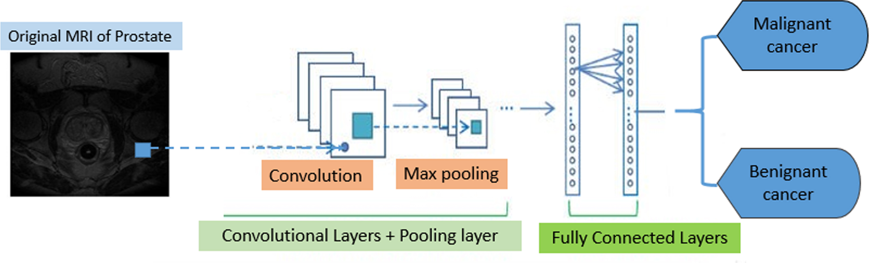
How a CNN works on the image and its classification. The input images go into feature extraction and classification, which are done by CNN. Specifically, after passing through the convolutional layers and the pooling layers, in the classification stage, the features extracted by the fully connected layers are divided into two classes, benign and malignant.

Figure 9 shows that the CNN network, with layers of convolution layers and pooling layer after extracting useful features in the last layer, performs the classification.

In recent years, deep learning has been extensively studied in various fields, and it has proved efficient [27]. Some studies also confirm that the use of CNN for extracting features in identifying targets is very distinct in the classification function; hence, a CNN model can be used as a starting point for teaching a new theme.

There are several popular CNN designs which simultaneously perform both steps of feature extraction and classification such as GoogleNet, ResNet18, ResNet50, and InceptionV3.

In the present study, two models of CNN are trained and all provide a comprehensive as well as complete answer due to the correct choice of preprocessing and zoning.

2.4.1 GoogleNet architecture

GoogleNet is an architecture designed by Google researchers [28]. Presenting the strongest model, GoogleNet was the winner of “ImageNet 2014”. In addition to a greater depth (22 layers) in this architecture, the researchers have also presented a new approach called the inception module. This module is a major change from the sequential architecture in which there were several types of “feature extractor” (layers that receive input values, and converting them into data for calculations) in a layer. In a network, which is learning and has to use several options for solving tasks, this type of layering indirectly contributes to a better network performance. This module can directly use inputs in its calculations, or directly summarize them. The final architecture consists of several modules that are stacked on top of each other. The method of learning is even different in GoogleNet since most upper layers have output layers. This minor change makes learning of this model faster as there are both general and parallel learning at the layers.

2.4.2 ResNet architecture

ResNet is a great architecture that shows how deep a deep learning architecture can be. ResNet [29] is an abbreviation of Residual Networks and consists of several sedimentary modules stacked on top of each other and they indeed constitute the main architectural structure of ResNet. In other words, a sediment module has two options, either it can perform a series of operations on the input, or it can skip all of these steps. As with GoogleNet, these sediment modules are stacked on top of each other to form a full network. The main advantage of ResNet is that thousands of these sediment layers can come together to form a network and then learn. This model is slightly different from normal sequential networks and does not have the problem of diminished performance in increasing the layers.

2.5 Evaluation parameters and results

The criteria obtained from the ROC curve [30] and confusion matrix [31] are the most important and common parameters for evaluating and comparing image tagging systems.

ROC curve for examining the ability and accuracy of models

Receiver operating characteristic (ROC) curve with receiving operating characteristics is a popular method of model evaluation. Roc is a criterion for measuring the efficiency in classification issues. This curve is widely used in signal detection theory, imaging system, radiological applications, and various fields of medicine such as cognitive tests and treatment regimens. ROC is indeed a graphical display of the degree of sensitivity (correct prediction) against the false prediction in a classification system where the separation threshold varies. The area under the ROC curve is a number that measures an aspect of efficiency and ranges from 0 to 1. The closer this number is to 1, the more accurate the prediction. Unlike other criteria for determining the efficiency of classifiers, the AUC criterion is independent of decision threshold of classifier. Thus, this criterion indicates the reliability of the output of a particular classifier for different data sets and cannot be calculated by other criteria for evaluating the efficiency of classifiers.

2.5.1 Confusion matrix

In classifying a data set using classification methods, the aim is to achieve the highest possible accuracy in classifying and identifying the classes. In some cases, it is more important for us to correctly detect the samples of a class. Confusion matrix has N*N dimensions where N is the number of optional classes. This matrix shows the function of a classification algorithm according to input data sets to separate different types of classes.

Each matrix element is defined as follows:

The number of records with negative real classes, with the classification algorithm also correctly detecting them with negative classes.

The number of records with positive real classes, with the classification algorithm also correctly detecting them with positive classes.

The number of records with negative real classes, with the classification algorithm also incorrectly detecting them with positive classes.

The number of records with positive real classes, with the classification algorithm also incorrectly detecting them with negative classes.

Sensitivity: It indicates the correct predicted value versus all positive outputs, and is also called the Recall, which is defined as follows: $Recall = TP / (TP + FN)$ (1)

Specificity: It indicates the correct negative predicted value versus all negative outputs. It is defined as follows: $Specificity = TN / (FP + TN)$ (2)

As with the accuracy criterion, these two parameters (sensitivity and specificity) are usually expressed in percentage. It is clear that an excellent prediction has both sensitivity and specificity of 100%.

Positive predictability: It indicates the number of correct positive predictions versus the number of all positively predicted items, which is defined as follows: $Precision = TP / (TP + FP)$ (3)

2.5.2 Accuracy

It is the most common, basic, and simplest criterion of the quality of a classifier and refers to the number of correct predictions versus all predicted items. This parameter indicates the number of patterns that are correctly detected, and is formulated as well as defined based on the matrix above as follows: $Accuracy = (TP + TN) / (TP + TN + FP + FN)$ (4)

2.5.3 F1-score

There is another important parameter called (F1-score) which is used to evaluate the performance of classifiers and is a combination of two parameters, sensitivity and positive predictability. $F 1 - score = 2 * (Recall * Precision) / (Recall + Precision)$ (5)

2.5.4 Dice similarity coefficient

Dice similarity coefficient (DSC): DSC is usually used to calculate the similarity of two images and is a principal criterion for evaluating the results of medical image segmentation. The DSC output is a number between 0 and 1, and the closer it is to 1, the more accurate the classification. The following equation presents the DSC value, which is defined as follows: $DSC = \frac{2 TP}{2 TP + FP + FN}$ (6)

3 Results and discussion

This part of the article presents the data set and the results obtained from applying the method.

Implementation was performed in MATLAB 2019b.

The input images belonged to 31 patients who were evaluated by a physician and divided into benign and malignant cancers. MRI images had T2 weights. Then, the number of images increased to 124 to augment data and improve the method’s strength in terms of accuracy. Next, the Faster R-CNN algorithm was applied to separate the prostate gland from the background image of MRI. At this stage, after training and testing the network, 115 identifiable images were obtained. Then, the image features were taken and divided into two categories of benign and malignant using two deep learning architectures. There are three options in CNN architecture: train data, test, and validation.

The train and test data ratio was 80 to 20, i.e. 80% of the images were considered for training and 20% for testing, and the validation was also drawn.

The following table presents the malignant cancers in the first group and benign prostate cancers in the second group.

Table 1 lists the results of using two different deep learning architecture. The results include sensitivity, specificity, precision, negative predictive rate, and accuracy.

Table 1
Results of applying two different networks, GoogleNet and ResNet18

Deep learning network Sensitivity Specificity Precision Negative predictive rate Accuracy

GoogleNet 100% 87.50% 93.80% 100% 95.70%

ResNet18 93.30% 100% 100% 88.90% 95.70%

Deep learning network	Sensitivity	Specificity	Precision	Negative predictive rate	Accuracy
GoogleNet	100%	87.50%	93.80%	100%	95.70%
ResNet18	93.30%	100%	100%	88.90%	95.70%

According to the results in Table 1, accuracy has given the same answer for the two architectures.

Table 2 compares the Recall and F-score criteria for two benign and malignant groups:

Table 2

Results for F1-score and Recall criteria with two selected methods: GoogleNet and ResNet18

Deep learning network	F1-score		Recall
	malignant	benign	Malignant	Benign
GoogleNet	96.77%	93.33%	100%	87.5%
ResNet18	96.55%	94.12%	93.33%	100%

According to Table 2, the diagnosis of benign and malignant cancer based on criteria F1-score and Recall with architecture ResNet18 had better results.

Figure 10 shows further results from the two selected architectures, including DSC, AUC, and ACCURACY.

Fig. 10

Calculation of DSC, AUC, and Accuracy criteria for ResNet18 and GoogleNet architectures.

With the results obtained in Fig. 10, It is obvious that the ResNet18 architecture has given the best answer in terms of accuracy.

Figure 11 reveals the confusion matrix for the two selected architectures.

Fig. 11

Calculation of confusion matrix for the selected architectures, GoogleNet and ResNet18; calculated by MATLAB software. (a) – calculation of confusion matrix for ResNet18 architecture. (b) – calculation of confusion matrix for GoogleNet architecture.

Figure 12 indicates the ROC Chart for the two selected architectures.

Fig. 12

Calculation of ROC Chart for two architectures, GoogleNet and ResNet18, calculated by MATLAB software. (a) – calculation of ROC Chart for ResNet18 architecture. (b) – calculation of ROC Chart for GoogleNet architecture.

The loss function diagram or cost function demonstrates the value of error each time the network is run for training data. Indeed, the task of the internal network is to learn the correct amount of weights and deviations in the network so that it can distinguish between different categories. In machine learning, this is done through iteration. Indeed, the data are given to the algorithm several times and each time the algorithm has to update its weight and bias value. In the first implementation of the deep learning algorithm, this algorithm gives a series of initial weight and deviation values to the vectors of weights and deviations so that these vectors have a series of initial values. Then, each time the deep learning network calculates its error, it updates the error values, weights, and deviations. This error calculation must be calculated by the cost function or the loss function. Indeed, the network learns how many times is should update weights and deviations by looking at the extent of damage it has done each time.

Figures 13 and 14 also illustrate the training process of the two architectures.

Fig. 13

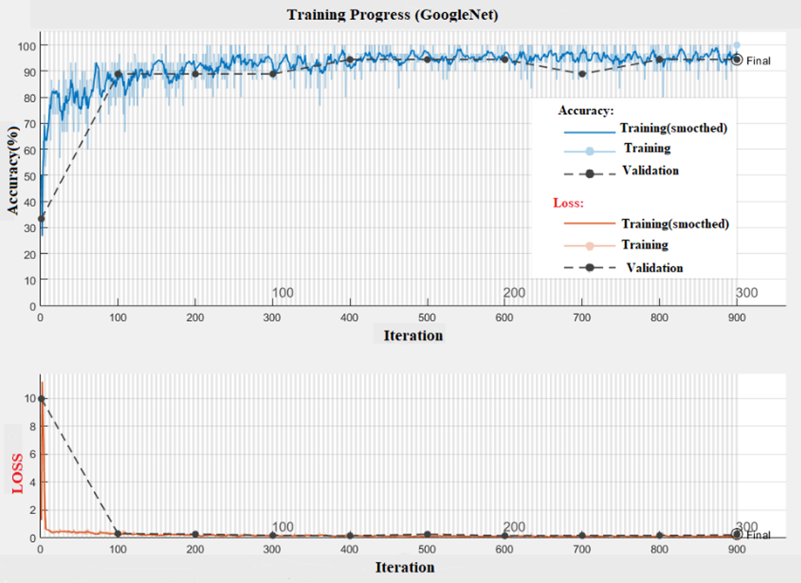
Training progress of GoogleNet architecture. Diagrams of changes in accuracy and loss are considered separately; in both diagrams, training (smooth) and general training as well as validation are also drawn separately.

Fig. 14

Training progress of ResNet18. Diagrams of changes in accuracy and loss are considered separately; in both diagrams, training (smooth) and general training and validation are also drawn separately.

Execution was done in MATLAB2019b software and in GPU, in the case of item iteration; the performance time of the two selected architectures was almost the same and each took about 17 minutes to run. They had and the item validation is 100% for both, but as seen, ResNet18 has had a more stable performance. The results obtained from the calculation of Recall and F1-score show that the architecture ResNet18 is more reliable. Meanwhile, the final answer of equal accuracy is worth considering for both architectures and shows that the selected steps in a row are correctly selected and located. Table 3 compares the AUC of recent methods and the proposed method.

Table 3

Comparison of AUC of the proposed method and AUC of previous works

Methods	Year	AUC
Li, M., et al. [36]	2020	0.98
Abraham et al. [15]	2019	0.74
Bonekmap et al. [32]	2018	0.89
Jiance Li et al. [33]	2018	0.91
The proposed method		0.9917

In [15], the segmentation of prostate cancer is based on the convolutional neural network using MRI images and LADTree classification. In the article [32] a comparison is made between the features of Radiomic machine learning and the features of the images obtained from ADC images. In the article [33], the evaluation of the performance of the support vector machine (SVM) for classifying the Gleason score (GS) of prostate cancer in the central gland (Central Gland) is performed based on the characteristics of multi-parametric MRI images. In [36] in order to diagnose prostate cancer, a model based on clinical trials using a radimics feature extracted from MRI images has been presented and a comparison between clinical methods and machine learning methods based on radimics features by plotting ROC It has been done.

Table 4 compares the DSC of recent methods and the proposed method.

Table 4

Comparison of DSC of the proposed method and DSC of previous works

Methods	Year	DSC
Hambarde, P., et al [37]	2020	0.8958
Zhenzh Dai [14]	2019	0.86
Minh nguyen [34]	2018	0.95
Tian et al. [35]	2017	0.853
The proposed method		0.9655

In [14], the R-CNN mask was used to segment the prostate mri images, and a comparison was made between the proposed method and the two-dimensional and three-dimensional U-net method. Then, by drawing the ROC diagram, the results were compared with other methods [34]. A three-dimensional CNN has been proposed for the multi-parametric MRI segmentation of prostate images that follows the encoder-decoder framework. In [35] an automatic segmentation method with CNNs for MRI images is introduced. In this work, images with T2 weight are used and then the results are analyzed by extracting Radiomic features and analyzing them by random forest. In [37], two-dimensional U-net convolution neural network and MR images with T2 weight were performed to segment the prostate gland and also to diagnosis the lesion and separate it from the rest of the image.

4 Conclusion

Our aim of this research was to achieve the ability of reaching the same answer for different methods, that is, each set of images given to this system would have the same answer, as obtained with accuracy = 95.7% from both methods. In this study, two methods of deep learning GoogleNet and ResNet18 were used whereby items AUC, Accuracy, and ROC were measured. According to the results, the architecture ResNet18 had a better performance. In previous research, either the cancer model has not been diagnosed or it has made more errors, while in this study, fewer errors were detected. One of the proposed solutions to continue this research is to use a deep learning network with fewer layers to enhance the speed of response. Low error in physician diagnosis can change the patient’s prognosis, so if an automated system can be provided for physicians with minimal error, it will be a huge step forward the future of medicine.

CRediT authorship contribution statement

The N.Pirzad-Mashak conceived the study, participated in its design and coordination, and helped produce the manuscript. The G. Akbarizadeh and E. Farshidi participated in the design and coordination and helped draft the version. All authors of the final version have read and approved the manuscript and agree with it.

Declaration of competing interest

The authors declare that they have no known competing financial interests or personal relationships that could have appeared to influence the work reported in this paper.

Footnotes

Acknowledgments

The work described in this paper was supported by the Shahid Chamran University of Ahvaz, as a PhD. thesis under Grant No. SCU.EE99.269. The authors would like to thank the Shahid Chamran University of Ahvaz for financial support.

Funding

Funding Name: Shahid Chamran University of Ahvaz, Funding Number: SCU.EE99.269

Availability of data and materials

The datasets used and/or analyzed during the current study are available from the corresponding author on reasonable request.

Contribution of authors

The N. Pirzad-Mashak conceived the study, participated in its design and coordination, and helped produce the manuscript. The G. Akbarizadeh and E. Farshidi participated in the design and coordination and helped draft the version. All authors of the final version have read and approved the manuscript and agree with it.

Consent for publication

All the authors have consented to the publication of this manuscript.

Competitive advantages

The authors participating in the study stated that they do so ‘do not have any conflict of interest with this version.

References

Siegel

R.L.

, Miller

K.D.

and Jemal

, Cancer statistics, CA Cancer J Clin 69(1) (2019), 7–34.

Crawford

E.D.

, Epidemiology of prostate cancer 62(6 SUPPL. 1) (2003), 3–12.

Wilson

K.M.

, Giovannucci

E.L.

and Mucci

L.A.

, Lifestyle and dietary factors in the prevention of lethal prostate cancer, Asian Journal of Andrology 14(3) (2012), 365–374. doi: 10.1038/aja.2011.142

Markozannes

, et al., Diet, body size, physical activity and risk of prostate cancer: An umbrella review of the evidence, European Journal of Cancer 69 (2016), 61–69. doi: 10.1016/j.ejca.2016.09.026

Yoneyama

, Komiyama

and Fujiwara

, Diagnosis of prostate cancer, IRYO – Japanese Journal of National Medical Services 57(11) (2003), 670–675. doi: 10.11261/iryo1946.57.670

Gaunay

, et al., Role of multi-parametric MRI of the prostate for screening and staging: Experience with over cases, Asian J Urol 4(1) (2017), 68–74. doi: 10.1016/j.ajur.2016.09.011

Artan

, Haider

M.A.

, Langer

D.L.

and Yetik

I.S.

, Semi-supervised prostate cancer segmentation with multispectral MRI, in 2010 IEEE International Symposium on Biomedical Imaging: From Nano to Macro, 2010, pp. 648–651.

You

J.Y.

, et al., Value of T1/T2-weighted magnetic resonance imaging registration to reduce the postbiopsy hemorrhage effect for prostate cancer localization, Prostate Int 3(3) (2015), 80–86. doi: 10.1016/j.prnil.2015.06.005

Yang

, Zhan

, Xie

, Zhao

and Kurihara

, Hierarchical prostate MRI segmentation via level set clustering with shape prior, Neurocomputing 257 (2017), 154–163.

10.

Soujanya Chilla

, Heng Tan

, Xu

and Loo Poh

, Diffusion weighted magnetic resonance imaging and its recent trend-a survey, Quant Imaging Med Surg 5(3) (2015), 407–422. doi: 10.3978/j.issn.2223-4292.2015.03.01

11.

The Radiology Assistant: Prostate Cancer – PI-RADS v2, https://radiologyassistant.nl/abdomen/prostate/prostate-cancer-pi-rads-v2 (accessed Aug. 24, 2020).

12.

Nelson

C.R.

, Ekberg

and Fridell

, Prostate Cancer Detection in Screening Using Magnetic Resonance Imaging and Artificial Intelligence, Open Artif Intell J 6(1) (2020), 1–11. doi: 10.2174/1874061802006010001

13.

Cuocolo

, et al., Machine learning for the identification of clinically significant prostate cancer on MRI: a meta-analysis, Eur Radiol 2020. doi: 10.1007/s00330-020-07027-w

14.

Dai

, et al., Segmentation of the Prostatic Gland and the Intraprostatic Lesions on Multiparametic MRI Using Mask-RCNN, 2019, [Online]. Available: http://arxiv.org/abs/1904.02575

15.

Abraham

and Nair

M.S.

, Computer-aided grading of prostate cancer from MRI images using Convolutional Neural Networks, J Intell Fuzzy Syst 36(3) (2019), 2015–2024. doi: 10.3233/JIFS-169913

16.

Prostate MR Image Database, http://prostatemrimagedatabase.com/ (accessed Aug. 22, 2020).

17.

Zalpour

, Akbarizadeh

and Alaei-Sheini

, A new approach for oil tank detection using deep learning features with control false alarm rate in high-resolution satellite imagery, Int J Remote Sens 41(6) (2020), 2239–2262. doi: 10.1080/01431161.2019.1685720

18.

Charmouti

, Junoh

A.K.

, Muhamad

W.Z.A.W.

, Mansor

M.N.

, Hasan

M.Z.

and Mashor

M.Y.

, Extended median filter for salt and pepper noise, Int J Appl Eng Res 12(22) (2017), 12914–12918.

19.

Kovesi

, Fast almost-Gaussian filtering, Proc. – 2010 Digit. Image Comput. Tech. Appl. DICTA 2010, pp. 121–125, (2010). doi: 10.1109/DICTA.2010.30

20.

Wong

C.Y.

, et al., Image contrast enhancement using histogram equalization with maximum intensity coverage, J Mod Opt 63(16) (2016), 1618–1629. doi: 10.1080/09500340.2016.1163428

21.

Wallach

, Developing, A World Made for Money, pp. 241–294, 2017. doi: 10.2307/j.ctt1d98bxx.10

22.

Doll

, et al., Mask r-cnn, in Proceedings of the IEEE international conference on computer vision, 2017, pp. 2961–2969.

23.

Girshick

, Fast R-CNN, Proceedings of the IEEE International Conference on Computer Vision 2015 Inter. (2015), 1440–1448. doi: 10.1109/ICCV.2015.169

24.

Carroll

, YOLO9000: Better, faster, stronger, Eur Pharm Contract no. SUMMER, p. 30, 2014. doi: 10.5860/lrts.53n4.261

25.

Liu

, et al., SSD: Single shot multibox detector, in Lecture Notes in Computer Science (including subseries Lecture Notes in Artificial Intelligence and Lecture Notes in Bioinformatics) 9905(LNCS) (2016), 21–37. doi: 10.1007/978-3-319-46448-0_2

26.

Deng

, Dong

, Socher

, Li

L.-J.

, Li

and Fei-Fei

, Imagenet: A large-scale hierarchical image database, in 2009 IEEE conference on computer vision and pattern recognition, 2009, pp. 248–255.

27.

Carneiro Neto

, Deep Learning Based Analysis of Prostate Cancer from MP-MRI, 2020.

28.

Zeng

, He

, Yu

, Yang

and Zhang

, Preparation of novel high copper ions removal membranes by embedding organosilane-functionalized multi-walled carbon nanotube, Journal of Chemical Technology and Biotechnology 91(8) (2016), 2322–2330. doi: 10.1002/jctb.4820

29.

Yun

J.W.

, Deep Residual Learning for Image Recognition arXiv:1512.03385v1, Enzyme Microb Technol 19(2) (1996), 107–117. doi: 10.1016/0141-0229(95)00188-3

30.

Streiner

D.L.

and Cairney

, What’s under the ROC? An introduction to receiver operating characteristics curves, Can J Psychiatry 52(2) (2007), 121–128. doi: 10.1177/070674370705200210

31.

Powers

D.M.W.

and Ailab, Evaluation: From Precision, Recall and F-Factor to ROC, Informedness, Markedness & Correlation, J Mach Learn Technol 2(December) (2007), 37–63. [Online]. Available: http://www.bioinfo.in/contents.php?id=51

32.

Bonekamp

, et al., Radiomic machine learning for characterization of prostate lesions with MRI: Comparison to ADC values, Radiology 289(1) (2018), 128–137. doi: 10.1148/radiol.2018173064

33.

, et al., Support Vector Machines (SVM) classification of prostate cancer Gleason score in central gland using multiparametric magnetic resonance images: A cross-validated study, Eur J Radiol 98(2) (2018), 61–67. doi: 10.1016/j.ejrad.2017.11.001

34.

M.N.N.

, Vu

D.Q.

, Turkbey

, Choyke

P.L.

and Kwak

J.T.

, Deep dense multi-path neural network for prostate segmentation in magnetic resonance imaging, Int J Comput Assist Radiol Surg 13(11) (2018), 1687–1696. doi: 10.1007/s11548-018-1841-4

35.

Tian

, Liu

and Fei

, Deep convolutional neural network for prostate MR segmentation, Med Imaging 2017 Image-Guided Proced Robot Interv Model 10135 (2017), 101351L, doi: 10.1117/12.2254621

36.

, et al., Radiomics prediction model for the improved diagnosis of clinically significant prostate cancer on biparametric MRI, Quantitative Imaging in Medicine and Surgery 10(2) (2020), 368.

37.

Hambarde

, et al., Prostate lesion segmentation in MR images using radiomics based deeply supervised U-Net, Biocybernetics and Biomedical Engineering 40(4) (2020), 1421–1435.

38.

Chandrasekaran, Gokul et al., Test Scheduling of System-on-Chip Using Dragonfly and Ant Lion Optimization Algorithms, Journal of Intelligent & Fuzzy Systems 40(3) (2021), 4905–4917. https://doi.org/10.3233/JIFS-201691

39.

Chandrasekaran

, Periyasamy

and Rajamanickam

K.P.

, Minimization of test time in system on chip using artificial intelligence-based test scheduling techniques, Neural Computing and Applications 32 (2020), 5303–5312. https://doi.org/10.1007/s00521-019-04039-6

40.