Unsound wheat kernel recognition based on deep convolutional neural network transfer learning and feature fusion

Abstract

Unsound wheat kernel recognition is an important part of wheat quality inspection, and it is also a key indicator to measure wheat quality. Research on unsound wheat kernel recognition is of great significance to the correct evaluation of wheat quality. The existing researches on unsound wheat kernel recognition are mainly to directly optimize the classical classification networks, and the recognition effect is often unsatisfactory due to insufficient training data. Aiming at the problem that the recognition rate of unsound wheat kernels is not ideal due to the lack of training data, we propose a Transfer Learning Feature Fusion (TLFF) model. The model uses transfer learning and feature fusion to identify unsound wheat kernels. First, feature extraction is performed by deep Convolutional Neural Networks (CNNs) VGG-16 and VGG-19 pre-trained on the large public dataset ImageNet. Then, the features extracted by the pre-trained neural networks are fused and classified through the flattening layer, fully connected layer, Dropout layer, and Softmax layer. We conduct experiments on single model, two-model fusion, three-model fusion, and four-model fusion, and select the three-model fusion scheme to perform this task. Finally, we vote on the output results of the three best fusion models to further improve the recognition rate. The pre-trained models we use are trained on a large public dataset ImageNet. Since the scale of the dataset is very large, these pre-trained models also have good generalization performance for images other than ImageNet dataset. Therefore, although our dataset is small, we can still achieve good recognition results. Experimental results show that the recognition performance of the TLFF model is significantly better than the existing unsound wheat kernel recognition models.

Keywords

Transfer learning feature fusion unsound wheat kernel recognition convolutional neural network voting

1 Introduction

Wheat is one of the three major cereals, which is widely planted in the world. Currently, wheat is planted around 2.2 million hectares worldwide, accounting for about 1/3 of the world’s total grain production. About 35% of the world’s people mainly eat wheat, and its consumption shows a global trend. Wheat is not only the main source of human food, but also an important industrial raw material. With the progress of society, a large number of wheat has gradually changed from grain consumption to industrial raw materials for processing food [1]. As an important part of global grain, wheat plays an important role in world grain production and trade, and it is the most traded grain. Therefore, wheat, as an important food crop and important commodity grain in the world, plays an important role in the production, circulation, and consumption of grain.

In the process of wheat production and trading, quality grading is a very important work. The unsound wheat kernel is an important indicator to measure the quality of wheat, and it is one of the most common problems in wheat quality inspection. The research on unsound wheat kernel recognition technology is of great significance for the correct evaluation of wheat quality [2]. In the purchase and circulation of wheat, the inspection of wheat mostly needs to be completed manually on the spot, and the classification of unsound wheat kernels can only be judged by the subjective judgment of human eyes. Manual inspection of wheat easily doped with more human factors, this method is cumbersome and labor-intensive. This method is easy to cause classification and grading errors due to the subjectivity of testers and visual fatigue, which brings great uncertainty to the quality classification of wheat [3].

Traditional machine learning methods require manual extraction of wheat features, which are too special to fully reflect the essential characteristics of wheat. The method of artificial feature extraction will produce a large number of characteristic parameters, which need to be optimized by Principal Component Analysis(PCA) and other methods. The process is cumbersome and the recognition effect is not ideal. In recent years, artificial intelligence has been widely applied and developed in agriculture [4, 5], industry [6, 7], remote sensing [8], medical care [9], and other fields. As an important technology of artificial intelligence, Convolutional Neural Networks (CNNs) have been widely used in construction [10], medical [11], transportation [12], video production [13, 14], and other industries. In the field of agriculture, Convolutional Neural Networks (CNNs) detect plant diseases by image recognition of leaves [15 –20] and fruits [21]. In addition, CNN models have also achieved good results in the field of face recognition [22], pedestrian detection [23], license plate recognition [24], and cheque handwritten number recognition [25]. Different from the traditional image recognition methods, CNN depth models avoid the feature extraction algorithm based on prior knowledge [26]. They have the advantages of autonomous learning and self-improvement, and the extracted features are more scientific and comprehensive. As important methods in the field of artificial intelligence, transfer learning and feature fusion can effectively improve the performance of the model. Transfer learning can accelerate the convergence speed of the model and effectively solve the problem that the recognition effect is not ideal due to the lack of training data. It is applied in emotion recognition [27], medicine [28], and fault diagnosis [29]. Feature fusion method can realize the complementary advantages of multiple features and make the features more identifiable. This method has been applied in transportation [30, 31] and industry [32 –34], and achieved good results.

There are three methods of unsound wheat kernel recognition. (1) Wheat features are manually extracted, and then the extracted features are input into a classification model for recognition. However, the features extracted by this method are often too special, the extracted feature information cannot well reflect the essential characteristics of wheat, and the extraction process is complicated. (2) Take special spectral images of wheat, and then input the images into the model for recognition. This method requires complex image preprocessing, which is time-consuming and has poor practicability. From the economic aspect, hyperspectral imaging equipment is expensive, and the cost of the matching detection equipment is also high. (3) Optimizing classical classification networks. For example, adding Dropout, pyramid pooling [35], and Batch Normalization (BN) layers to regular CNN. These methods require training weights from the first layer of the model. At present, there is no large public dataset of unsound wheat kernels, and the dataset size is usually small. Therefore, although the classical classification model is optimized, the recognition effect is still not ideal.

Although existing methods have achieved good results in unsound wheat kernel recognition, these methods still have the following problems. (1) These methods all need to be trained from the first layer of the model, and the recognition rate is often unsatisfactory due to the small size of the unsound wheat kernel dataset. (2) The extracted wheat feature information is not comprehensive. Although the classical CNN is optimized, the wheat feature information extracted by a single model is usually not comprehensive enough. To address these issues, we propose the Transfer Learning Feature Fusion (TLFF) model. Aiming at the problem that the recognition rate is not ideal due to the small size of the unsound wheat kernel dataset, we introduce the idea of transfer learning [36]. Aiming at the problem that the wheat feature information extracted by a single model is not comprehensive, we adopt the method of multi-model feature fusion. The TLFF model uses the pre-trained models VGG-16 and VGG-19 of the ImageNet dataset to extract wheat features, and fuse the acquired features. Finally, we introduce the voting mechanism in ensemble learning to further improve the recognition rate by voting on the recognition results of the three fusion models.

The major contributions of this paper are:

(1) We introduce transfer learning idea into unsound wheat kernel recognition. Different from the existing unsound wheat kernel recognition models, we use the pre-trained models of large public dataset to extract wheat feature. This method can still extract high-quality features with less training data. Compared with models without transfer learning, our model has better generalization performance.

(2) We fuse the features extracted by multiple models. Different from the existing single model feature extraction methods in unsound wheat kernel recognition tasks, we use multiple models for feature extraction. Then the features extracted from multiple models are fused. The wheat feature information contained in the fusion features is more comprehensive and abundant, making the feature more identifiable.

(3) We introduce the voting mechanism in ensemble learning to integrate the results of multiple fusion models. The voting mechanism is used to improve the output results, so that the recognition rate is further improved. Our proposed TLFF model outperforms other baseline models on the unsound wheat kernel recognition tasks.

The rest of the paper is organized as follows. Section 2 describes the related work. Section 3 first describes the problem of unsound wheat kernel recognition and propose key definitions, and then introduces our TLFF model in detail. Section 4 discusses the experimental setup and results. Section 5 concludes the paper and discusses future work.

2 Related work

2.1 Methods for unsound wheat kernel recognition

The unsound wheat kernel is an important indicator to measure the quality of wheat and an important basis for the grading of wheat in the wheat market circulation. In order to improve the accuracy of unsound wheat kernel recognition, many scholars have made great efforts for this work and published many academic works, which promoted the development of this field. The methods of unsound wheat kernel recognition are mainly divided into three categories: unsound wheat kernel recognition based on artificial extraction features, unsound wheat kernel recognition based on hyperspectral image, and unsound wheat kernel recognition based on deep learning.

2.1.1 Unsound wheat kernel recognition based on artificial extraction features

The early unsound wheat kernel recognition was mainly to extract color, morphology, and texture features by artificial method, and then input the extracted features into the model for classification. Luo et al. [37] input the extracted color features and morphological features of wheat grains into a secondary discriminant classifier and a K-nearest neighbor classifier for identification. Singh et al. [38] extracted color, morphology, and texture features of wheat, and then input the extracted feature parameters into three statistical discriminant classifiers and a neural network classifier. Chen [39] extracted 178 wheat features and sent them to Support Vector Machine(SVM) for classification. Neethirajan et al. [40] input the extracted 17 wheat features into statistical classifier and neural network classifier to classify wheat. Zhang et al. [41] input the extracted 54 color, morphology, and texture features into the BP neural network. Zhu et al. [42] photographed seven kinds of wheat images, extracted the color, morphology, and texture features of wheat, and sent them to BP neural network for classification. Although the method of manually extracting features have achieved good results in unsound wheat kernel recognition, the extracted features are usually too special. The features extracted by artificial method cannot fully reflect the essential characteristics of wheat.

2.1.2 Unsound wheat kernel recognition based on hyperspectral image

Image quality has a great influence on the unsound wheat kernel recognition. In order to make wheat features more obvious, some scholars try to obtain hyperspectral images of wheat. Yu et al. [2] took hyperspectral images of four kinds of wheat and classified them through a CNN model. Hao et al. [43] fused hyperspectral images and high resolution images of wheat, and used fused images as data sources to identify wheat. Yu et al. [44] used a hyperspectral imaging system to take hyperspectral images of wheat to achieve non-destructive detection of unsound wheat kernels. Dong et al. [45] combined the spectral features and image features of hyperspectral image to improve the recognition rate. Liu et al. [46] took hyperspectral images of seven kinds of wheat, and transported hyperspectral images to MobileNet V2 network for recognition. Liu et al. [47] took hyperspectral reflectance images of four kinds of wheat, and identified the images through the established model, and achieved good recognition results. Although the method of unsound wheat kernel recognition based on hyperspectral image has been widely used in the research, it still stays in the laboratory test stage. Hyperspectral imaging equipment is expensive and post-processing is very complex.

2.1.3 Unsound wheat kernel recognition based on deep learning

Unsound wheat kernel recognition method based on deep learning solves the research bottleneck of traditional machine learning methods in the field of wheat quality detection. The neural network uses the original images as input, which can effectively learn the corresponding features from a large number of samples, avoiding the complex feature extraction steps. Zhu et al. [48] compared SVM, BP neural network, and convolutional neural network. The experimental results show that the recognition effect of convolutional neural network is better. Zhang et al. [49] adopted the VGG16 neural network under the Keras framework as the recognition model of unsound wheat kernels. In order to improve the model performance, some scholars have optimized conventional neural network models. He et al. [50] added Batch Normalization (BN) layer to the classical classification neural networks LeNet5, ResNet-34, and VGG-16 respectively for optimization, and achieved good classification results. Cao et al. [51] added a pyramid pooling layer to the conventional CNN, and its recognition rate was improved compared to the conventional CNN. Zhang [52] added residual block and Batch Normalization algorithm to the classic CNN model to improve the performance of the model. The wheat features extracted by neural network are more scientific and comprehensive than those obtained by manual extraction method. Although deep learning has become the mainstream method for unsound wheat kernel recognition, the problem of unsatisfactory recognition rate due to the small size of the dataset still exists.

2.2 The latest researches on plant disease recognition

Recently, some scholars have conducted in-depth researches in the field of plant diseases and applied artificial intelligence to plant disease recognition. Almadhor et al. [53] manually extracted the color and texture features of guava leaves, and then input the extracted features into a machine learning classifier for disease recognition. Abayomi-Alli et al. [54] synthesized cassava images through image color histogram transformation technology, and then used MobileNetV2 neural network to realize cassava disease detection. Oyewola et al. [55] balanced cassava leaf dataset by block processing technology, and detected cassava mosaic disease by residual neural network. Kundu et al. [56] extracted the image features of pearl millet farmland by transfer learning method, and realized the intelligent detection of pearl millet disease. Du et al. [57] used CNN model to detect tomato leaf diseases, and made the model have good recognition performance through feature fusion method. Liu et al. [58] photographed hyperspectral images of three leaves of Dangshan pear, and transported the extracted characteristic wavelengths to SPA-SVM model for disease recognition. Su et al. [59] introduced the idea of transfer learning, and constructed the grape leaf disease recognition model based on VGG-16. In order to further improve the recognition effect, some scholars have improved conventional neural networks. Wang et al. [60] proposed an improved CenterNet-SPP model, which shortened the training time and improved the F1 value. Bao et al. [61] improved the CNN by randomly discarding some neurons and their connections, and combined the Inception module and the ResNet module for feature extraction of corn leaf images. Liu et al. [62] improved the SqueezeNet model by changing the network structure to improve the recognition rate of leaf diseases. Xiang et al. [63] obtained the Xception_CEMs model by introducing the CEM module on the basis of Xception, which effectively improved the recognition effect of the model. Shi et al. [64] improved the residual neural network by feature fusion and structure reduction, which improved the recognition efficiency of the model. Yue et al. [65] improved the model by adding high-order residual and parameter sharing feedback sub-network into the VGG network, which effectively enhanced the robustness of the model. Zhu et al. [66] improved convolution kernel based on traditional residual neural network and introduced SE attention mechanism. Huang et al. [67] designed the VGG19-INC model on the basis of the VGG19 network model. They improved the VGG19 model by transfer learning, multi-scale feature fusion, and full connection layer transformation, which effectively improved the generalization performance of the model. Fan et al. [68] used L2 regularization and Dropout method to improve the convolutional neural network, which effectively improved the recognition ability of the model.

2.3 Problems with existing methods and motivation for this study

Although existing methods have achieved good results in unsound wheat kernel recognition task, there are still some problems. (1) The researches on unsound wheat kernel recognition have not solved the problem of poor recognition rate due to the small size of the wheat dataset. At present, the transfer learning method has not been used in the unsound wheat kernel recognition task to solve the problem that the recognition effect is not ideal due to the small size of the dataset. Transfer learning method has recently been applied in intelligent detection of pearl millet diseases. However, this study did not perform feature fusion on the high-quality features extracted by the pre-trained models in order to obtain better detection results. Transfer learning method has been applied in citrus pest recognition and grape leaf disease recognition, but these studies are based on a single model, and do not realize the complementary advantages of multiple models. (2) The existing methods still have the problem that the extracted wheat feature information is not comprehensive. The existing unsound wheat kernel recognition methods still focus on one type of model for feature extraction, so the phenomenon of incomplete feature information is inevitable. Feature fusion method has been applied in tomato leaf disease detection, which uses unsupervised Canonical Correlation Analysis (CCA) algorithm for feature fusion. Unsupervised Canonical Correlation Analysis (CCA) algorithm ignores the label information, so the discriminant of fusion features is not too strong. In the studies of silkworm disease recognition and citrus disease recognition, researchers realized feature fusion by modifying the model structure. These studies still use a single model for feature extraction, and do not achieve multi-feature complementary advantages.

Given the problems with existing methods, we propose a TLFF model for this purpose. The TLFF model adopts the transfer learning method to solve the problem of unsatisfactory recognition rate due to the small size of the wheat dataset. The problem that the extracted wheat feature information is not comprehensive is improved by the feature fusion method. Finally, the voting mechanism in ensemble learning is introduced to further improve the recognition rate.

There are two differences between prior works and the solution presented in this paper. (1) Compared to prior works, we effectively solve the problem that the recognition rate is not ideal due to the lack of training data by transfer learning method. We use the pre-trained neural networks of ImageNet, a large public dataset, to extract features. Because of its large scale, its pre-trained models also have good generalization ability for images outside the dataset. Transfer learning method can still extract good quality features in the case of less training data, so as to effectively solve the problem of poor recognition rate caused by less training data. In prior works, the models need to be trained from the first layer, and the recognition effect is often unsatisfactory due to the lack of training data. (2) The prior works are to extract features of wheat through a single model, and the extracted feature information comes from the mining of a single model. The feature information extracted by a single model is usually not comprehensive, and the recognition effect is often not ideal. We adopt the multi-model feature fusion method, that is, the features extracted by multiple models are fused in a concatenating manner. Different models can mine different feature information, and the multi-model feature fusion method can realize the complementary advantages of multi-feature and make the feature more identifiable.

In order to further present differences between existing unsound wheat kernel recognition works and the solution presented in this paper, we compare them from four aspects, as shown in Table 1. It can be seen from Table 1 that among the four items compared, the performance of the model proposed in this paper is the best. Firstly, the feature extraction steps of the proposed method are simple and the feature quality is good. Secondly, the proposed method in this paper effectively solves the problem of poor recognition effect caused by less training data and single model feature extraction, which has not been well solved in prior works.

Table 1
Comparison of existing methods with the method proposed in this paper

Unsound wheat kernel recognition methods Feature extraction steps Quality of features Insufficient training data leads to unsatisfactory recognition rate Feature information extracted by single model is incomplete

Unsound wheat kernel recognition

based on artificial extraction features Complex Not very good Unsolved Unsolved

[37 –42]

Unsound wheat kernel recognition

based on hyperspectral image Complex High-quality Unsolved Unsolved

[2 , 43–47]

Unsound wheat kernel recognition

based on deep learning Simple Good Unsolved Unsolved

[48 –52]

TLFF Simple High-quality Effectively solved Effectively solved

Use pictures as (1)Use pictures as

Solutions input data directly. input data directly; Transfer learning Multi-model feature fusion

(2)Feature fusion.

Unsound wheat kernel recognition methods	Feature extraction steps	Quality of features	Insufficient training data leads to unsatisfactory recognition rate	Feature information extracted by single model is incomplete
Unsound wheat kernel recognition
based on artificial extraction features	Complex	Not very good	Unsolved	Unsolved
[37 –42]
Unsound wheat kernel recognition
based on hyperspectral image	Complex	High-quality	Unsolved	Unsolved
[2 , 43–47]
Unsound wheat kernel recognition
based on deep learning	Simple	Good	Unsolved	Unsolved
[48 –52]
TLFF	Simple	High-quality	Effectively solved	Effectively solved
	Use pictures as	(1)Use pictures as
Solutions	input data directly.	input data directly;	Transfer learning	Multi-model feature fusion
		(2)Feature fusion.

3 Model

In this section, we first describe the problem of unsound wheat kernel recognition, and then introduce each part of the TLFF model. The overall architecture of the TLFF model is shown in Fig. 1, which includes four parts: transfer learning (feature extraction), feature fusion, classification, and voting. We use the VGG backbone network to build the TLFF model, which has the characteristics of small convolution kernel and multi convolution sublayer. The VGG network uses multiple convolution layers with smaller convolution kernels to replace a convolution layer with larger convolution kernels. On the one hand, parameters can be reduced. On the other hand, it is equivalent to more nonlinear mapping, which can increase the fitting ability of the network. To improve the readability of the paper, we list the abbreviations and their full names in this paper in Table 2.

Fig. 1

The architecture of our proposed Transfer Learning Feature Fusion (TLFF) model.

Table 2

Abbreviation comparison table

Abbreviation	Full name
TLFF	Transfer learning feature fusion
CNN	Convolutional neural network
BN	Batch normalization
SVM	Support vector machine
CCA	Canonical correlation analysis
SPP	Spatial pyramid pooling
SGD	Stochastic gradient descent
BP	Back propagation
IE	Image enhancement
RGB	Red green blue
TP	True positive
FP	False positive
FN	False negative

3.1 Problem formulation

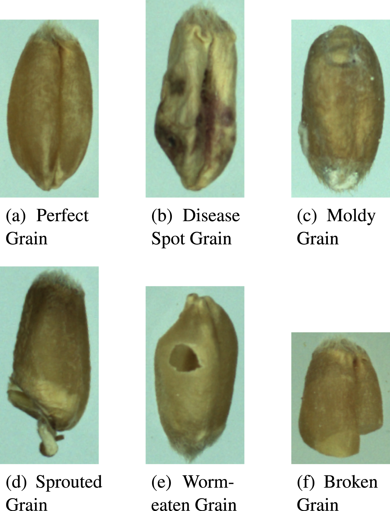
Unsound wheat kernel recognition: The wheat image is input into the established model, and then the model judges the identified wheat category according to the characteristic information reflected in the wheat image. The six types of wheat are shown in Fig. 2.

Fig. 2

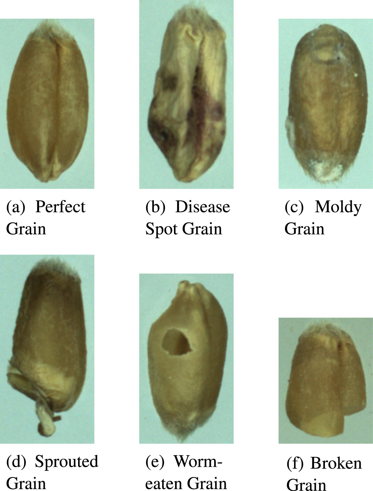
Images of six types of wheat.

3.2 Transfer learning

Transfer learning is the first part of the TLFF model. The TLFF model retains the convolution layers and pooling layers of the pre-trained models, and replaces the original top layers with the self-designed top layers. The self-designed top layers include the flattening layer, full connection layer, Dropout layer, and Softmax layer. During the training process, only the self-designed top layers are trained. The pre-trained model is used to extract wheat features, and the extracted features are sent to the self-designed top layers for classification.

Transfer learning can be defined as: Given a source domain D_S and learning task T_S, a target domain D_T and learning task T_T, transfer learning aims to help improve the learning of the target predictive function f_T (.) in D_T using the knowledge in D_S and T_S, where D_S≠D_T, or T_S≠T_T.

3.3 Feature fusion

Feature fusion is the second part of the TLFF model. We use feature fusion method to concatenate the features extracted from multiple models to make the extracted feature information more comprehensive. The shapes of the extracted features of the pre-trained models VGG-16 and VGG-19 are both (None, 7, 7, 512), and then the function “concatenate()” is used to perform array concatenation on the extracted features. “concatenate ()” is a very useful array operation function, which can complete the concatenation of multiple arrays at one time. Its main function is to concatenate a series of arrays along an axis, and the incoming arrays must have the same shape. We concatenate along the direction of axis=-1, that is, concatenate the last dimension. Taking three features of shape (None, 7, 7, 512) as input, feature concatenating is performed along the last dimension, and the output shape is (None, 7, 7, 1536).

In this task, the three fusion models we used (Fusion Model 1, Fusion Model 2, Fusion Model 3) are as follows.

Fusion Model 1: The 512-dimensional features extracted from each of the two VGG-16 networks and the VGG-19 network are concatenated together into 1536-dimensional fusion features. This is shown in Table 3.

Table 3
The case of fusion model 1

Model VGG-16 VGG-16 VGG-19

Output (None, 7, (None, 7, (None, 7,

shape 7, 512) 7, 512) 7, 512)

Fusion shape (None, 7, 7, 1536)

Model	VGG-16	VGG-16	VGG-19
Output	(None, 7,	(None, 7,	(None, 7,
shape	7, 512)	7, 512)	7, 512)
Fusion shape	(None, 7, 7, 1536)

Fusion Model 2: The 512-dimensional features extracted from each of the two VGG-19 networks and the VGG-16 network are concatenated together into 1536-dimensional fusion features. This is shown in Table 4.

Table 4

The case of fusion model 2

Model	VGG-16	VGG-19	VGG-19
Output	(None, 7,	(None, 7,	(None, 7,
shape	7, 512)	7, 512)	7, 512)
Fusion shape	(None, 7, 7, 1536)

Fusion Model 3: The 512-dimensional features extracted from each of the three VGG-16 networks are concatenated together into 1536-dimensional fusion features. This is shown in Table 5.

Table 5

The case of fusion model 3

Model	VGG-16	VGG-16	VGG-16
Output	(None, 7,	(None, 7,	(None, 7,
shape	7, 512)	7, 512)	7, 512)
Fusion shape	(None, 7, 7, 1536)

3.4 Classification

Classification is the third part of the TLFF model, including flattening layer, fully connected layer, Dropout layer, and Softmax layer. The flattening layer is located between the convolutional layer and the fully connected layer, and expands the multi-dimensional data into one-dimensional data to facilitate the data processing of the fully connected layer.

In the case of too many parameters and too few training samples, the neural network model is prone to overfitting [69]. To prevent overfitting, we add Dropout algorithm to the model, which allows one neuron to work with other randomly selected neurons. The overfitting phenomenon of deep neural networks can be alleviated by breaking the interdependence of neurons. This method weakens the joint adaptability between neuron nodes and enhances the generalization ability [70].

The classifier used in TLFF model is Softmax classifier. The Softmax classifier normalizes the output data of the previous layer, and then selects the node corresponding to the maximum value as the prediction result. The calculation formula is shown in Equation (1). $y_{im} = \frac{e^{z_{im}}}{\sum_{k = 1}^{K} e^{z_{ik}}}$ (1) where y_im is the predicted probability that the ith sample belongs to the mth class, K is the number of classes, z_im is the product of the output vector of the ith sample and the parameter vector of the mth class, and z_ik is the product of the output vector of the ith sample and the parameter vector of the kth class.

In this task, we use categorical_crossentropy as the loss function, and its calculation formula is shown in Equation (2). $L = - \sum_{i = 1}^{n} {\hat{y}}_{im} \lg y_{im}$ (2) where n is the batch size, L is the loss function, and ${\hat{y}}_{im}$ is the expected probability that the ith sample belongs to the mth class.

3.5 Voting

Voting is the fourth part of the TLFF model. We adopt the hard voting method, whose principle is to select the label with the most output by the algorithm, and select them in ascending order if the number of labels is equal. The schematic diagram of the voting process is shown in Fig. 3.

Fig. 3

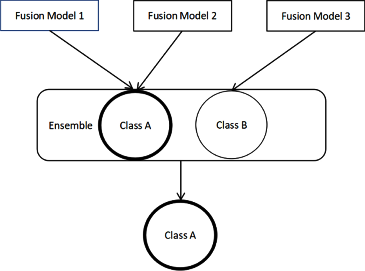
Voting process.

We vote on the outputs of the three fusion models ((i.e., Fusion Model 1, Fusion Model 2, and Fusion Model 3). Experiments show that Fusion Model 1 has the highest recognition accuracy rate (96.0%) among the three models, Fusion Model 2 has the second highest recognition rate (95.9%), and Fusion Model 3 has the lowest recognition rate (95.7%). Our voting criteria are as follows: When two models have the same prediction result, and the third has a different prediction result, the predicted results of the two models will be used as the final prediction result. If all three prediction results are the same, this result will be used as the final prediction result. If all prediction results are different, the prediction result of Fusion Model 1 will be used as the final prediction result.

4 Experiments

4.1 Experimental settings

4.1.1 Dataset

The dataset we use includes perfect grains and five types of unsound grains (i.e., perfect grains, disease spot grains, moldy grains, sprouted grains, worm-eaten grains, and broken grains). The wheat samples are manually sorted for sample selection and classification.

The acquisition device of wheat images in this task is composed of a shaking automatic feeding tray, a transparent carrier plate, and a pair of high-definition industrial cameras. In this way, high-definition RGB images of wheat are obtained.

We use multi-grain wheat that are not sticking to each other and flat on a plane as the original images collection object. Therefore, the original images are multi-grain wheat images, and their states are shown in Fig. 4. We need to perform image segmentation on the original images, and segment the images into images with only single grain wheat in each image. In this paper, the contour detection algorithm is used to segment multi-grain wheat images into single-grain wheat images. Take the rectangular area determined by the edge of the wheat grain as the boundary, expand 3 pixels to the surrounding area, and then crop. The segmented images are shown in Fig. 5.

Fig. 4

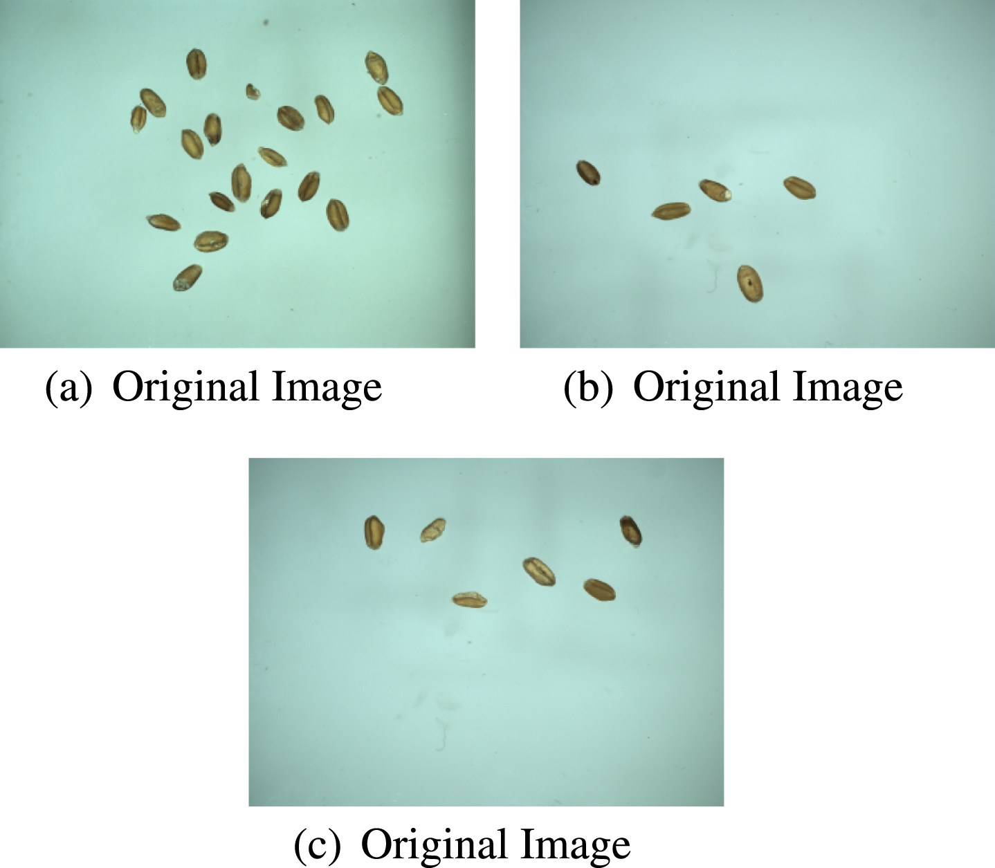
Original images of wheat.

Fig. 5

Grain images after segmentation.

We use a contour detection algorithm to segment the original wheat images into images with only singlegrain wheat in each image. First convert the wheat image to grayscale. Then use Canny operator to extract wheat edges. Next, detect the minimum circumscribed rectangle of the contour, expand it by 3 pixels, and then crop it. The Canny operator is not susceptible to noise interference and can detect real weak edges. It can detect strong edge and weak edge using two different thresholds. The implementation process of Canny operator is as follows [71]:

(1)Perform convolution with a 2D Gaussian filter template to eliminate noise.

(2) Use the derivative operator to find the partial derivative (G_x, G_y) of the image gray along the two directions, and find the magnitude $| G | = \sqrt{G_{x}^{2} + G_{y}^{2}}$ (3) of the gradient.

(3) Use the result of (2) to calculate the direction $Θ = Arctan (\frac{G_{x}}{G_{y}})$ (4) of the gradient.

(4) The gradient direction of the edge can be roughly divided into four types: the horizontal direction, the vertical direction, the 45-degree direction, and the 135-degree direction. Using these directions, the neighboring pixels can be found.

(5) Traverse the image. If the gray value of a certain pixel is not the largest compared to the gray value of the two pixels before and after the gradient direction, then the pixel value is set to 0; that is, it is not an edge.

(6) Use the cumulative histogram to calculate two thresholds: a high threshold and a low threshold. The one greater than the high threshold must be an edge, and the one less than the low threshold must not be an edge. In between, determine if there are edge pixels that exceed the high threshold; any pixels exceeding the threshold comprise an edge.

A database is established based on the segmented single-grain wheat images. We collected 2782 images of each type of wheat (i.e., 2782 images of perfect grains, 2782 images of disease spot grains, 2782 images of moldy grains, 2782 images of sprouted grains, 2782 images of worm-eaten grains, and 2782 images of broken grains). Among them, 2000 images are used as training set, 400 images are used as validation set, and 382 images are used as test set.

In practical applications, the lighting effect when taking an image cannot be guaranteed to be absolutely uniform, and noise is inevitably introduced. Therefore, we perform data augmentation on images in the training set using strategies of varying brightness and introducing Gaussian noise. In this way, the generalization ability of the TLFF model is improved. The training set is therefore expanded from the original 2000 images per category to 4000 images per category. Figure 6 shows partially enhanced wheat images.

Fig. 6

Enhanced wheat images.

Table 6

Main notations used in this section

Variables	Description
G _x	Difference in horizontal direction
G _y	Difference in vertical direction
Θ	The direction of the gradient

4.1.2 Evaluation method

In this task, we use hold-out method to evaluate the model. The hold-out method directly divides the dataset D into two mutually exclusive sets, one of which is used as the training set S, and the other is used as the test set T, that is, D = S ∪ T,S ∩ T = φ.After training the model on S, we use T to evaluate the error.

In this task, we divide the 2782 images of each class of wheat into three sets that are mutually exclusive. Among them, 2000 images are used as training set, 400 images are used as validation set, and 382 images are used as test set. We expand the 2000 training set images to 4000 images through the data enhancement method. Therefore, we train the model on 24000 images in the training set, and use 2400 images in the verification set to evaluate the error. At the end of each round of training and verification, only the current best model is saved. After all rounds of training, we use the best saved model to make prediction on the 2292 images in the testing set.

We use the validation set loss value (val_loss) as the evaluation index. Meanwhile, we use the cross_entropy loss function categorical_crossentropy to evaluate the difference between the current training probability distribution and the true distribution, which is defined as follows: $C = - \frac{1}{n} \sum_{x} [ylna + (1 - y) \ln (1 - a)]$ (5) where y is the expected output, a is the actual output of the neuron, and c is the loss value.

4.1.3 Evaluation metrics and experimental parameter settings

In this task, we use Precision (P), Recall (R), and the harmonic mean (F1) of precision and recall as metrics to evaluate the effect of recognition. True Positive (TP) refers to the number of positive samples that are correctly classified. False Positive (FP) refers to the number of negative samples that are incorrectly labeled as positive samples. False Negative (FN) refers to the number of positive samples that are incorrectly marked as negative samples. The specific evaluation process is shown in Equations (6)–(8). $P = \frac{TP}{TP + FP} \times 100 %$ (6) $R = \frac{TP}{TP + FN} \times 100 %$ (7) $F 1 = \frac{2 \times P \times R}{P + R} \times 100 %$ (8)

Precision and recall are two evaluation metrics widely used in computer science to evaluate the performance of models. Precision and recall are contradictory in many cases, which requires a parameter that can comprehensively consider these two indicators, which is the F1 value. The three indicators of Precision, Recall, and F1 value are used for model evaluation at the same time, which can make a scientific and reasonable evaluation of the model.

We adjust the parameters according to the accuracy and loss during each training process. Our model is implemented based on Keras 2.4.3. In order to prevent the model from overfitting, we add Dropout and L2 regularization in the training phase. An excessive learning rate makes it difficult for the model to converge. If the learning rate is too small, the convergence speed will be too slow. In order to solve these two problems, we adopt a decreasing learning rate, setting the initial learning rate to 0.0008 and the decreasing rate to 0.00002. Set the Batch Size to 16, Dropout to 0.5, and Momentum to 0.9. To prevent overfitting, we employ an Early Stopping method to stop training the network. After 30 iterations, if the recognition effect of the model on the validation set does not improve, the training is stopped immediately. When the performance of the model on the validation set does not improve, the Early Stopping method can stop the training of the model, thereby preventing overfitting.

4.2 TLFF model data and comparative experiments

4.2.1 TLFF model data

There are three transfer learning feature fusion models in the TLFF model: VGG-16+VGG-16+VGG-19 model, VGG-16+VGG-19+VGG-19 model, and VGG-16+VGG-16+VGG-16 model. The parameter quantity and parameter distribution of the three models are shown in Tables 7, 8, and 9.

Table 7
Parameter quantity and distribution of VGG-16+VGG-16+VGG-19 model

Layer Number of parameters

VGG-16 Model 14714688

VGG-16 Model 14714688

VGG-19 Model 20024384

Layer	Number of parameters
VGG-16 Model	14714688
VGG-16 Model	14714688
VGG-19 Model	20024384

The total number of parameters of the VGG-16+VGG-16+VGG-19 model is 49453760, and the number of trainable parameters is 49453760.

Table 8

Parameter quantity and distribution of VGG-16+VGG-19+VGG-19 model

Layer	Number of parameters
VGG-16 Model	14714688
VGG-19 Model	20024384
VGG-19 Model	20024384

The total number of parameters of the VGG-16+VGG-19+VGG-19 model is 54763456, and the number of trainable parameters is 54763456.

Table 9

Parameter quantity and distribution of VGG-16+VGG-16+VGG-16 model

Layer	Number of parameters
VGG-16 Model	14714688
VGG-16 Model	14714688
VGG-16 Model	14714688

The total number of parameters of the VGG-16+VGG-16+VGG-16 model is 44144064, and the number of trainable parameters is 44144064.

The number of images in the original training set is 2000 for each category of wheat, and the data augmentation method is used to expand to 4000 for each category. The number of validation set images for each type of wheat is 400, and the number of test set images for each type of wheat is 382. Overall, the training set has 24,000 images, the validation set has 2,400 images, and the test set has 2,292 images.

The TLFF model is run on a machine with 64 GB RAM, Intel i7-6800 K CPU, and NVIDIA TITAN Xp GPU. The input image size of the model is 256 × 256. When the TLFF model runs, it occupies 1.1035 GB memory. The running time of VGG-16+VGG-16+VGG-19 model is 0.6051 s, the running time of VGG-16+VGG-19+VGG-19 model is 0.6134 s, and the running time of VGG-16+VGG-16+VGG-16 model is 0.5824 s. The running time of voting on the three fusion models is 1.5219 s. Therefore, the running time of TLFF model is 3.3228 s.

4.2.2 Comparative experiments

(1) Comparison with recently developed models

We evaluate the TLFF model by four new models for unsound wheat kernel recognition and three new models for disease recognition. The recognition results on our dataset are shown in Table 10.

VGG-16+IE+BN [50] is a model that adds a Batch Normalization (BN) layer to the VGG-16 network. Image Enhancement (IE) is performed on wheat images, and then the enhanced images are sent to this model for recognition.

RseNet+BN [52] is a model that introduces residual block structure and BN algorithm based on the classical CNN model structure.

AlexNet [48] is a typical convolutional neural network.

VGG-16 [49] is a neural network with 13 convolutional layers, 5 pooling layers, and 3 fully connected layers, with strong deep learning ability.

The improved ResNet50 [64] is a neural network that partially modifies ResNet50 by feature fusion and structure reduction.

The improved VGG [65] is a model that adds the high-order residual and parameter sharing feedback sub-network into the VGG network.

VGG19-INC [67] is an improved model based on VGG19. The model takes VGG19 network model as the backbone network and uses transfer learning to realize the sharing of pre-trained weight parameters. Model structure improvement measures: (1) Replace the fifth convolution layer of VGG19 with one batch standardized convolution layer and two Inception modules; (2) A global pooling layer is used to replace the full connection layer of the VGG19 model; (3) Use a 1 × 4 Softmax layer as the classification output layer.

Table 10
Comparison with recently developed models

Model Precision/% Recall/% F1/%

VGG-16+IE+BN 91.53 92.45 91.98

RseNet+BN 89.94 92.13 91.02

AlexNet 83.23 85.17 84.18

VGG-16 85.32 86.75 86.02

Improved ResNet50 85.21 87.16 86.17

Improved VGG 87.43 88.89 88.15

VGG19-INC 89.17 90.91 90.03

TLFF 96.36 97.83 97.08

Model	Precision/%	Recall/%	F1/%
VGG-16+IE+BN	91.53	92.45	91.98
RseNet+BN	89.94	92.13	91.02
AlexNet	83.23	85.17	84.18
VGG-16	85.32	86.75	86.02
Improved ResNet50	85.21	87.16	86.17
Improved VGG	87.43	88.89	88.15
VGG19-INC	89.17	90.91	90.03
TLFF	96.36	97.83	97.08

The recently developed unsound wheat kernel recognition models do not adopt the transfer learning algorithm, so they need to start training from the first layer of the neural network. Due to the small size of the dataset, the recognition effect is not ideal. Although the models VGG-16 + IE + BN and RseNet + BN optimize the classical neural networks, they are still based on the feature extraction of a single model, so the extracted wheat feature information is not comprehensive. The TLFF model adopts the transfer learning method, which effectively solves the problem that the recognition rate is not ideal due to the small size of the dataset. It also uses multiple models to extract features and fuse them, so that the feature information is more abundant and the recognition effect is improved. Finally, the voting mechanism in ensemble learning is introduced to further improve the recognition rate. The TLFF model outperforms the other 4 models in precision, recall, and F1 value. This proves that the TLFF model outperforms the recently developed unsound wheat kernel recognition models.

The three newly developed disease recognition models are based on the classical model to improve the network structure. The improved ResNet50 and the improved VGG do not use the transfer learning method, because the number of samples used for training model is small, so their recognition effect is not ideal. The VGG19-INC model adopts the transfer learning algorithm to improve the generalization performance of the model, and the F1 value increases by 3.86 % and 1.88 % compared with the improved models of ResNet50 and VGG, respectively. TLFF model is superior to the three latest disease identification models in accuracy, recall, and F1 value. Therefore, the performance of TLFF model is superior to that of the recently developed disease recognition models.

(2) Comparison with other fusion models

In order to further verify the effectiveness of the proposed fusion method, we compare the fusion method in this paper with other fusion methods.

VGG-16+ Feature Pyramid [43] is an improved VGG-16 neural network model by feature pyramid. The wheat feature image fusion is realized by adding feature pyramid.

SVM+Feature Fusion [45] is a model that fuses spectral features and image features of wheat and then inputs them into SVM.

It can be seen from Table 11 that the F1 value of the TLFF model is 4.91% higher than that of the VGG-16+Feature Pyramid model and 13.56% higher than that of the SVM+Feature Fusion model. Both the VGG-16+Feature Pyramid and SVM+Feature Fusion models use a feature fusion method based on a single type of neural network. The TLFF model is based on feature fusion of different types of neural networks. Feature fusion of different types of models can effectively improve the richness of feature information. Experiments show that the recognition effect of multi-type model for feature fusion is better than that of single-type model.

Table 11

Comparison with other fusion models

Model	Precision/%	Recall/%	F1/%
VGG-16+Feature Pyramid	91.35	93.02	92.17
SVM+Feature Fusion	82.61	84.47	83.52
TLFF	96.36	97.83	97.08

(3) Comparison with other pre-trained models

In order to further verify the superiority of the pre-trained models used in this paper, we compare the VGG-16 and VGG-19 pre-trained models we used with other pre-trained models. The recognition results on our dataset are shown in Table 12.

Table 12

Comparison with other pre-trained models

Model	Precision/%	Recall/%	F1/%
Pre-trained AlexNet	84.69	86.58	85.62
Pre-trained ResNet50	85.72	87.03	86.37
Pre-trained DenseNet201	85.81	87.13	86.46
Pre-trained VGG-16	86.15	88.67	87.39
Pre-trained VGG-19	87.64	89.52	88.57

It can be seen from the comparison results that among the above pre-trained models, the AlexNet neural network has the smallest depth. Although its training speed is fast, its ability to extract features is weak. The DenseNet201 and ResNet networks are large in scale, and they are prone to over-fitting in the recognition tasks with small datasets. It can be seen from Table 12 that the F1 value of the pre-trained model of the VGG backbone network is about 1.5% higher than that of the ResNet50 and DenseNet201 pre-trained models. The F1 value of the pre-trained model of the VGG backbone network is about 2% higher than that of the AlexNet model. Experiments show that the pre-trained model of the VGG backbone network is more suitable for performing this task of unsound wheat kernel recognition.

(4) Comparison with the classic models

In order to further verify the superiority of the TLFF model compared to the classical models, we compare the TLFF model with three representative classical models. The recognition results on our dataset are shown in Table 13.

Table 13

Comparison with the classic models

Model	Precision/%	Recall/%	F1/%
Inception V3	85.32	86.17	85.74
ResNet 50	85.14	86.59	85.85
MobileNet	85.13	86.72	85.91
TLFF	96.36	97.83	97.08

It can be seen from Table 13 that the precision of the three classical models is about 85.20 %, the recall rate is about 86.50 %, and the F1 value is about 85.80 %. TLFF is superior to three classical neural networks in terms of precision, recall, and F1 value. TLFF model adopts transfer learning and feature fusion methods. Transfer learning can effectively solve the problem that the recognition effect is not ideal due to the lack of training data. It extracts better features by pre-trained models on large public datasets. Feature fusion can achieve complementary advantages of multiple features, and thus effectively improve the quality of feature information. Experiments show that the F1 value of TLFF model is about 11.25 % higher than that of the three classical models, and its recognition performance is better than that of classical models.

(5) The effectiveness of the methods used in the TLFF model

To demonstrate the effectiveness of transfer learning method, feature fusion, and data augmentation method, we conduct four groups of experiments. The first group is the VGG-16 model used by Zhang et al. [49]. The second group is the pre-trained model of VGG-16 on the ImageNet dataset. The third group is VGG-16+VGG-19 feature fusion model, and uses the feature fusion method used in this paper. The fourth group is the VGG-16 model that uses the data augmentation method used in this paper to augment the training set. The performance of these models on our dataset is shown in Table 14.

Table 14

Comparison of recognition results of different models

Model	Precision/%	Recall/%	F1/%
VGG-16	85.32	86.75	86.02
Pre-trained VGG-16	86.15	88.67	87.39
VGG-16+VGG-19	85.94	86.89	86.41
VGG-16(Data augmentation)	85.76	87.02	86.38

It can be seen from Table 14 that the precision of the VGG-16 model after data augmentation is increased by 0.44%, and the recall rate is increased by 0.27%, indicating that the data augmentation method used in this paper can effectively improve the recognition effect of the model. The data of the pre-trained model of VGG-16 is higher than that of the VGG-16 model in terms of precision, recall, and F1 value, which verifies the superiority of the transfer learning method we used. The F1 value of the VGG-16+VGG-19 model is 0.39 % higher than that of the VGG-16 model. The experimental results show that the feature fusion method used in this paper can effectively improve the performance of the model.

To verify the effectiveness of the voting method and the learning rate decreasing method used in this paper, we conduct comparative experiments on five models. The first is the VGG-16+IE+BN model adopted by He et al. [50]. The second is the RseNet+BN model adopted by Zhang [52]. The third model is a feature fusion model of two pre-trained neural networks on the large public dataset ImageNet. The fourth is a model that votes on the outputs of the three models above, and adopts the voting method used in this paper. The fifth model is to change the fixed learning rate of the second model to the learning rate decreasing method used in this paper, setting the initial learning rate to 0.0008 and the decreasing rate to 0.00002.

It can be seen from Table 15 that the Voting model is better than the previous three models in terms of precision and recall. The F1 value of the Voting model is 0.42% higher than that of the Pre-trained VGG-16+Pre-trained VGG-16 model. Experiments show that the voting method can effectively improve the model performance. The F1 value of the RseNet+BN model using the learning rate decreasing method is 0.92% higher than the original model, which proves the effectiveness of this method.

Table 15

Comparison of recognition results of different models

Model	Precision/%	Recall/%	F1/%
VGG-16+IE+BN	91.53	92.45	91.98
RseNet+BN	89.94	92.13	91.02
Pre-trained VGG-16+	91.35	93.02	92.17
Pre-trained VGG-16
Voting	91.98	93.21	92.59
RseNet+BN(Decreasing	91.76	92.13	91.94
learning rate)

(6)Significant difference analysis between TLFF model and baseline models

In order to further demonstrate the significant differences in performance between the TLFF model and the existing models for unsound wheat kernel recognition and disease recognition, we conduct the Anova test. We choose the F1 value that can take into account the two factors of precision and recall rate for comparison. TLFF model is compared with the six existing unsound wheat kernel recognition models and three disease recognition models. A total of 9 groups of comparative experiments are conducted, and the TLFF model and baseline model in each group are averaged after 3 experiments. The F1 values of different models are shown in Table 16. The Anova test results are shown in Table 17.

Table 16

F1 values of the TLFF model and the baseline models

Groups	TLFF(F1/%)	Baselines(F1/%)
1	97.08	91.98(VGG-16+IE+BN)
2	98.69	91.02(RseNet+BN)
3	95.01	84.18(AlexNet)
4	96.05	86.03(VGG-16)
5	97.24	92.17(VGG-16+Feature Pyramid)
6	96.57	83.52(SVM+Feature Fusion)
7	97.12	86.15(Improved ResNet50)
8	97.52	88.09(Improved VGG)
9	97.01	90.11(VGG19-INC)

Table 17

Anova test results. ” / ” represents that there is no data here, and these places in the table generated by the Anova test are spaces

Sources of	SS (sum of squared	df (degrees of	MS (mean	F (effect term/	P-value	F crit
difference	deviations)	freedom)	square)	error term)
Between groups	347.07342	1	347.07342	57.36811	1.12E-06	4.493998
Inside the group	96.79898	16	6.04994	/	/	/
Total	443.87240	17	/	/	/	/

It can be seen from Table 17 that the P value is 1.12E-06, which is less than 0.05, so there is a significant difference between the groups. This proves that the performance of the TLFF model is significantly better than that of the baseline models. In addition, many experiments can maintain a good recognition effect, which fully shows that the performance of the TLFF model is stable.

4.3 Online application

Although some calculations such as modeling unsound wheat kernel recognition can periodically be carried out offline, the continuous addition of wheat images necessitate short intervals under real conditions. We propose a strategy based on incremental update without full recalculation to suit online application.

For the TLFF model proposed in this paper, the main time complexity comes from the calculation of image files. The time complexity of TLFF model is approximately expressed as $O (| T |)$ , where T is an image set.

In the next calculation, we check whether new images are added. u is a single image, t′ is the set of new images, where t ∈ T and |t′| << |T|.

If u ∈ t′, then recalculate the Category (u). In this case, the time complexity is about $O (| t^{'} |)$ .

If u ∈ T - t′, then u is directly expressed as Category (u), that is, the previous calculation results need not be recalculated.

Therefore, when adding new images, the corresponding time complexity is $O (| t^{'} |)$ . Compared with the strategy based on recalculation, this method only needs to predict the new images, and the time cost is greatly reduced. In general, due to |t′| << |T|, the complexity of our incremental updating strategy is significantly reduced. Therefore, the complexity of TLFF model is fundamentally reduced to allow online application.

Time complexity: When considering new images, the time complexity of TLFF model is $O (| T | + | t^{'} |)$ .

Proof: Suppose T is the image set, u is a single image, t′ is the set of new images, where t ∈ T and |t′| << |T|. The time complexity of TLFF model without additional images is $O (| T |)$ .

When u ∈ t′, Category (u) is recalculated. The time complexity is about $O (| t^{'} |)$ .

When u ∈ T - t′, the previous calculation results are directly used, and u is directly expressed as Category (u) without recalculation.

In summary, when the TLFF model considers new images, the corresponding time complexity is $O (| T |) + O (| t^{'} |)$ , that is, $O (| T | + | t^{'} |)$ .

4.4 Model selection

In this section, we will describe the process of selecting the best model. At the same time, we will show the verification results of different models on our dataset to explain why we finally choose the TLFF model. The VGG-16 and VGG-19 models used in this section are pre-trained neural networks in large public dataset ImageNet.

4.4.1 Single transfer learning model

Since the VGG backbone networks have good performance in image recognition, we decide to adopt the VGG backbone networks. In order to solve the problem that the recognition rate is not ideal due to the small size of the wheat dataset, we choose the pre-trained model on ImageNet as the wheat feature extractor. Figure 7 is a schematic diagram of a single transfer learning model.

Fig. 7

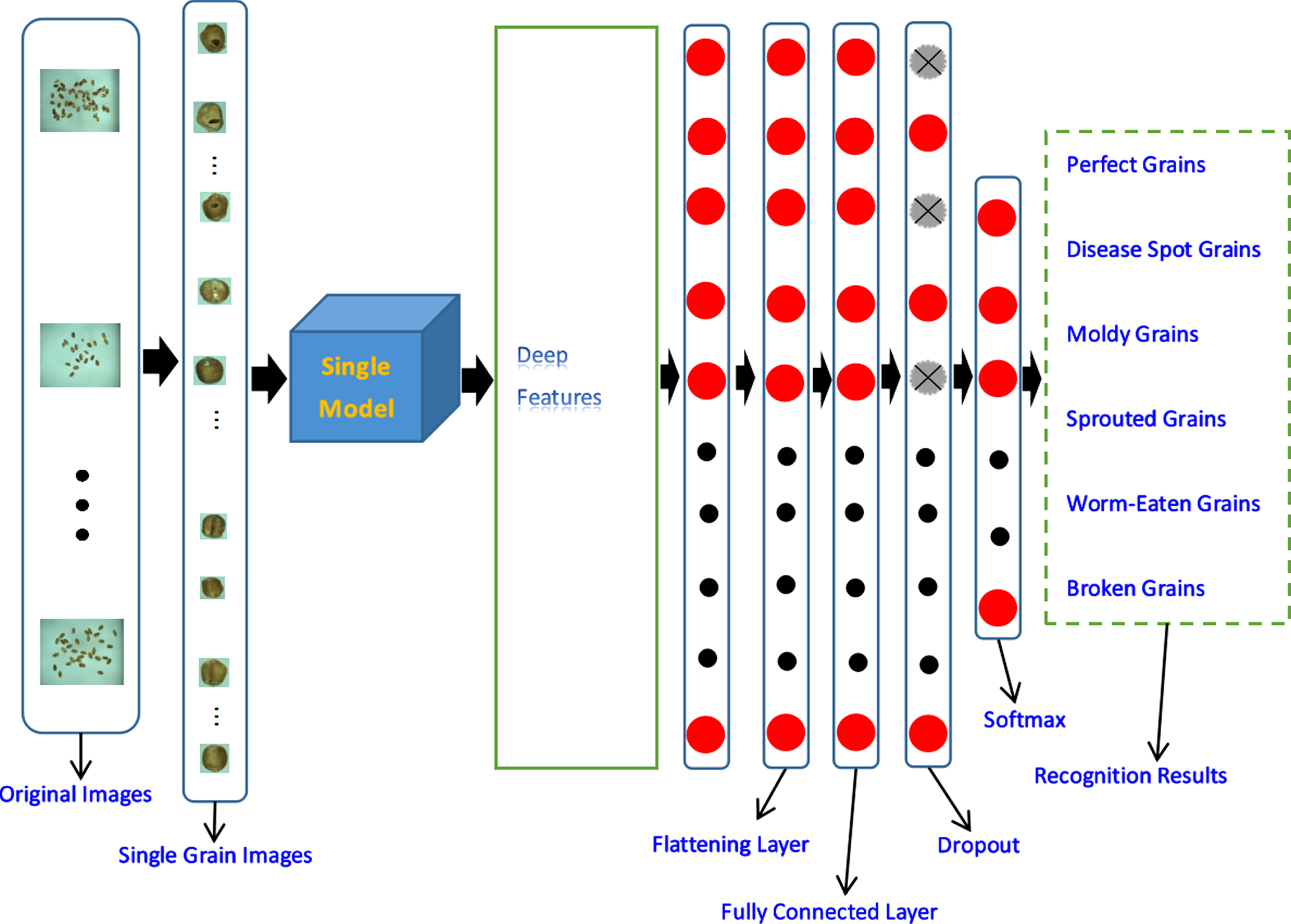
Single transfer learning model, where the “Single model” in Fig. 7 can be replaced with the pre-trained “VGG-16” or “VGG-19”.

The performance of VGG-16 and VGGG-19 pre-trained models on the dataset is shown in Fig. 8. It can be seen from the figure that the average value of the six experiments of the VGG-16 transfer learning model is 87.4%. The average value of six experiments for the VGG-19 transfer learning model is 88.6%. Thus, the average recognition rate of a single transfer learning model is about 88.0%.

Fig. 8

Performance of single transfer learning model, where the “Average Recognition Rate” in Fig. 8 refers to the average recognition rate of the six types of wheat (i.e., perfect grains, disease spot grains, moldy grains, sprouted grains, worm-eaten grains, and broken grains).

Experiments show that the extraction effect of a single model for wheat features is not ideal. The feature information extracted by a single model is often not comprehensive enough, and poor recognition rate is inevitable.

4.4.2 Fusion of two transfer learning models

Experiments show that the recognition effect of a single transfer learning model is not ideal, so we adopt the method of feature fusion of two transfer learning models to further improve the recognition rate. We construct three groups of two-model fusion: (1) The fusion of the features of the VGG-16 and VGG-19 pre-trained models. (2) The fusion of the features of the two VGG-16 pre-trained models. (3) The fusion of the features of the two VGG-19 pre-trained models. Figure 9 is the fusion model diagram of two pre-trained models. The performance of the above three fusion models on the dataset is shown in Fig. 10. The average of six experiments of VGG-16+VGG-19 model is 93.4 %. The average of six experiments of VGG-16+VGG-16 model is 92.2 %. The average recognition rate of VGG-19+ VGG-19 model is 93.1 %. In summary, the average recognition rate when fusing two transfer learning models is about 93.0%.

Fig. 9

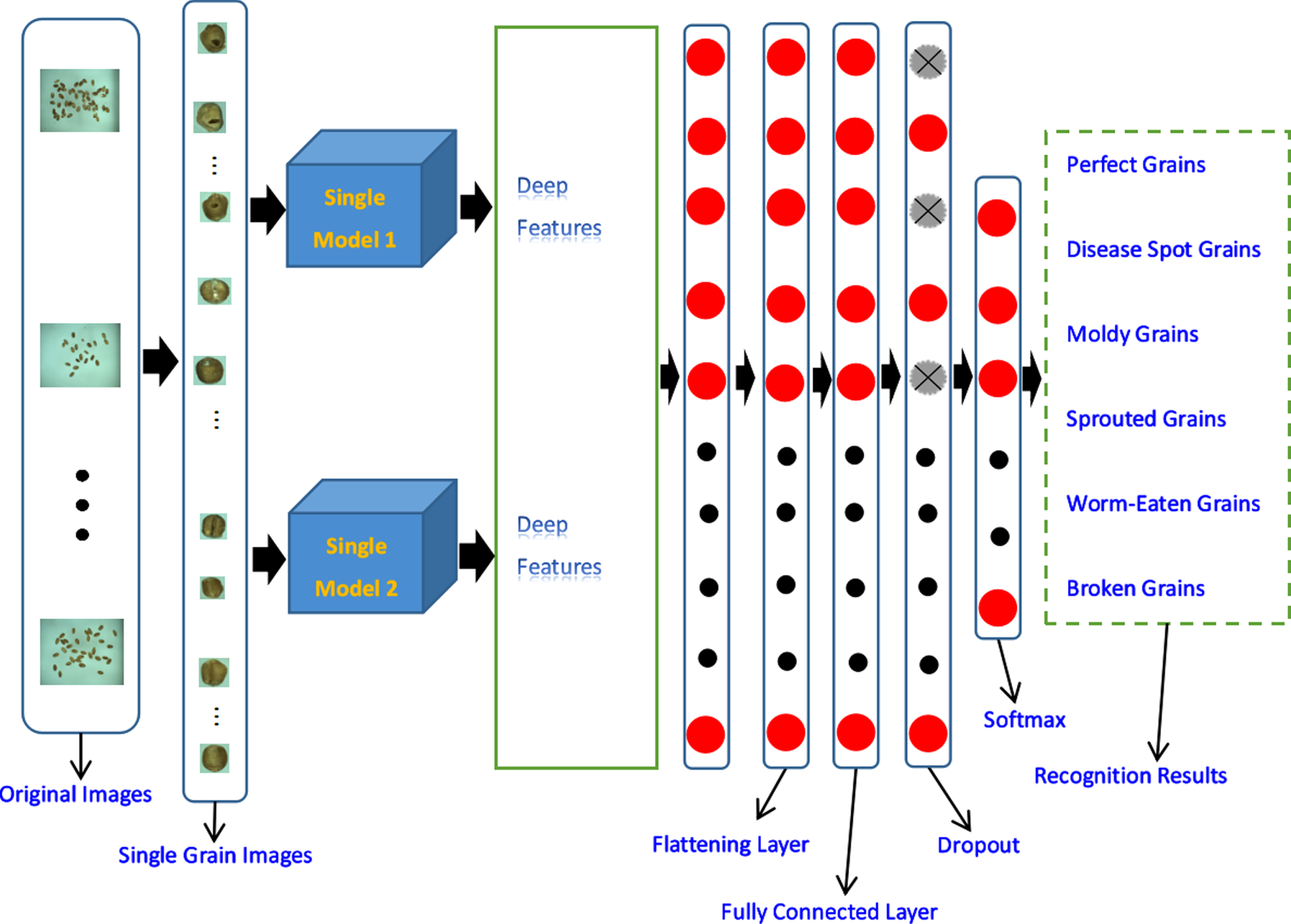
Two transfer learning models fused together, where the “Single model” in Fig. 9 can be replaced with the pre-trained “VGG-16” or “VGG-19”.

Fig. 10

Performance of two transfer learning models fused together, where the “Average Recognition Rate” in Fig. 10 refers to the average recognition rate of the six types of wheat (i.e., perfect grains, disease spot grains, moldy grains, sprouted grains, worm-eaten grains, and broken grains).

Experiments show that the recognition rate after fusion of the two models is about 5% higher than that of a single model. Because the wheat feature information contained in the fusion features is more comprehensive, it can better reflect the essential characteristics of wheat. Therefore, its recognition effect is significantly better than that of a single model.

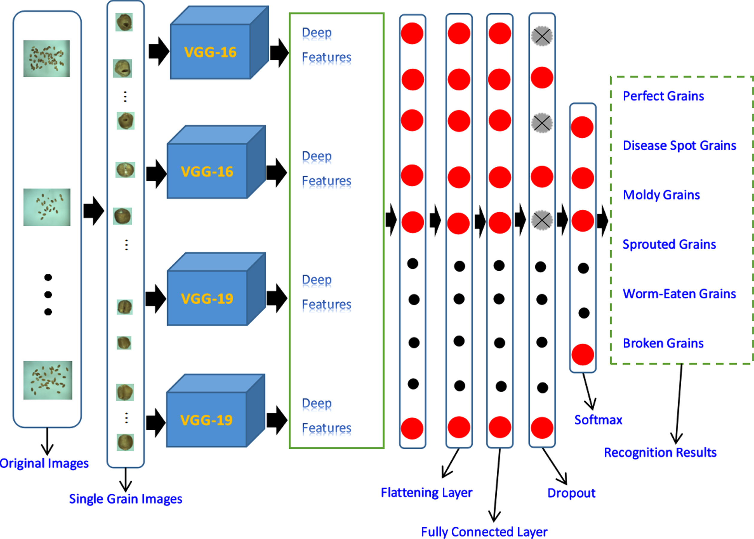
4.4.3 Fusion of three transfer learning models

To further improve the recognition rate, we fuse the three pre-trained models. We design four fusion models. The first group is VGG-16+VGG-19+VGG-19 model. The second group is VGG-16+VGG-16+VGG-19 model. The third group is VGG-19+VGG-19+VGG-19 model. The fourth group is VGG-16+VGG-16+VGG-16 model. Figure 11 is a schematic diagram of three-model fusion. The average values of the six experiments of the four transfer learning fusion models are 95.9 %, 96.0 %, 94.7 % and 95.7 %, respectively, as shown in Fig. 12. In summary, the average recognition rate of three-model fusion is about 95.5%. Experiments show that the recognition effect of the three models after fusion is better than that of the two models.

Fig. 11

Three transfer learning models fused together, where the “Single model” in Fig. 11 can be replaced with the pre-trained “VGG-16” or “VGG-19”.

Fig. 12

Performance of three-transfer learning fusion model, where the “Average Recognition Rate” in Fig. 12 refers to the average recognition rate of the six types of wheat (i.e., perfect grains, disease spot grains, moldy grains, sprouted grains, worm-eaten grains, and broken grains).

The output shapes of the features extracted by the pretrained models VGG-16 and VGG-19 are both (None, 7, 7, 512). We use the function “concatenate()” to concatenate the features extracted from the three models. “concatenate()” can complete the concatenation of multiple arrays at one time, and its main function is to concatenate a series of arrays along a certain axis. Three features of shape (None, 7, 7, 512) are used as input, feature concatenating is performed along the last dimension, and the output shape is (None, 7, 7, 1536). The network structure after concatenating is shown in Fig. 11. The convolutional layers and pooling layers of the three models are three independent parts, and they are fused by feature concatenating. Specifically, the three models perform feature extraction independently of each other. Then the features extracted from them are concatenated and input into the following network layers for classification.

4.4.4 Fusion of four transfer learning models

Next, we explore the fusion of the four models. We note from the previous section that the recognition rate is highest when both VGG-16 and VGG-19 are in the fusion model. Therefore, we combine two VGG-16 and two VGG-19 models for feature fusion, and the model is shown in Fig. 13. The average recognition rate of six experiments is 92.1%, as shown in Fig. 14. Since the recognition rate of four-model fusion is significantly lower than that of three-model fusion, we no longer further do the four-model fusion experiment.

Fig. 13

Fusion of VGG-16, VGG-16, VGG-19, and VGG-19 models.

Fig. 14

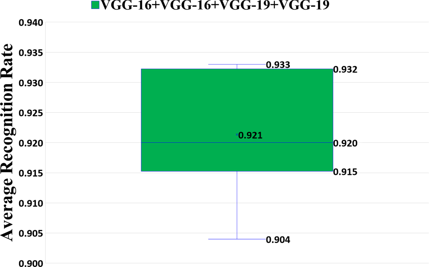
Performance of four transfer learning models fused together, where the “Average Recognition Rate” in Fig. 14 refers to the average recognition rate of the six types of wheat (i.e., perfect grains, disease spot grains, moldy grains, sprouted grains, worm-eaten grains, and broken grains).

Experiments show that the recognition rate of the four-model fusion does not increase but decrease. Because the wheat dataset is not large but the model is complex, the model is over-fitting and the performance of the model is degraded.

4.4.5 Voting

The voting method is a combination strategy for classification problem, and its basic idea is to select the class with the most output in the algorithm. Hard voting is to select the label with the most output. If the number of labels is equal, it is selected in ascending order. To further improve the recognition rate, we introduce an ensemble learning strategy to vote on the classification results of the three models by hard voting. The three models are already trained models, also known as “base model”. The recognition rate of the three base models for this task are between 95.5% and 96.0%, and the recognition effects are close, so it is suitable to use the voting method to improve the recognition rate. Among the three models we choose, the recognition accuracy of VGG-16+VGG-16+VGG-19 model is the highest, and the recognition rate is 96.0 %. The recognition rate of VGG-16+VGG-19+VGG-19 model is 95.9 %. The recognition accuracy of VGG-16+VGG-16+VGG-16 model is the lowest, and its recognition rate is 95.7 %. The specific voting criteria are: (1) Among the three models, when two models have the same prediction result and the other has different prediction result, the result predicted by the two models will be used as the final prediction result. (2) When the prediction results of the three models are consistent, this result is regarded as the final prediction result. (3) When the prediction results of the three models are different from each other, the prediction result of the VGG-16+VGG-16+VGG-19 model is used as the final result. The voting method is a commonly used method in ensemble learning, which reduces the variance through the integration of multiple models, thereby improving the robustness of the model. The three trained individual learners are finally formed into a strong learner through the combination strategy of hard voting, in order to achieve the purpose of learning from others’ strong points. Therefore, the purpose of improving the recognition rate can be achieved.

The above experiments prove that the three-model fusion has the best effect, and thus we optimize the model by voting on the results of the three transfer learning models fused together. The result after voting is 0.6% higher than the VGG-19+VGG-16+VGG-16 model with the highest recognition rate, and the recognition rate reaches 96.6%. Experiments show that the TLFF model has the best performance, so we decide to use this model to perform this task.

4.5 Influence of parameters

In this section, we report the results on our dataset to show our parameter tuning process, and then study the influence of some important hyperparameters.

4.5.1 Dropout ratio

Dropout is an effective method to prevent model overfitting. The key idea of Dropout method is to randomly drop units (along with their connections) from the neural network during training. This prevents units from co-adapting too much. This method weakens the joint adaptability between neurons and enhances the generalization ability of the model. Figure 15 shows the effect of dropout ratio on the average recognition rate of TLFF. TLFF has the highest recognition rate when the dropout ratio is equal to 0.5.

Fig. 15

Impact of dropout ratio on average recognition rate of the TLFF model, where the “Average Recognition Rate” in Fig. 15 refers to the average recognition rate of the six types of wheat (i.e., perfect grains, disease spot grains, moldy grains, sprouted grains, worm-eaten grains, and broken grains).

Experiments show that the TLFF model has the best recognition effect when dropout ratio is 0.5. Because when dropout ratio is 0.5, the network structure generated randomly is the most.

4.5.2 Regularization

Regularization is an effective means to control model complexity and reduce model overfitting. L1 regularization can produce a sparse model, which can prevent overfitting to a certain extent. Meanwhile, L2 regularization avoids model overfitting by limiting the size of the model W norm. We conduct experiments using L1 regularization and L2 regularization. Figure 16 shows the effect of L1 regularization on the average recognition rate of the TLFF model, and Fig. 17 shows the effect of L2 regularization on the average recognition rate of the TLFF model. We find that the average recognition rate of the TLFF model when using L1 regularization is 26.2%, and the average recognition rate of the TLFF model when using L2 regularization is 93.2%. When L2 is equal to 0.001, the average recognition rate of the TLFF model is the highest. Therefore, we set the L2 parameter to 0.001.

Fig. 16

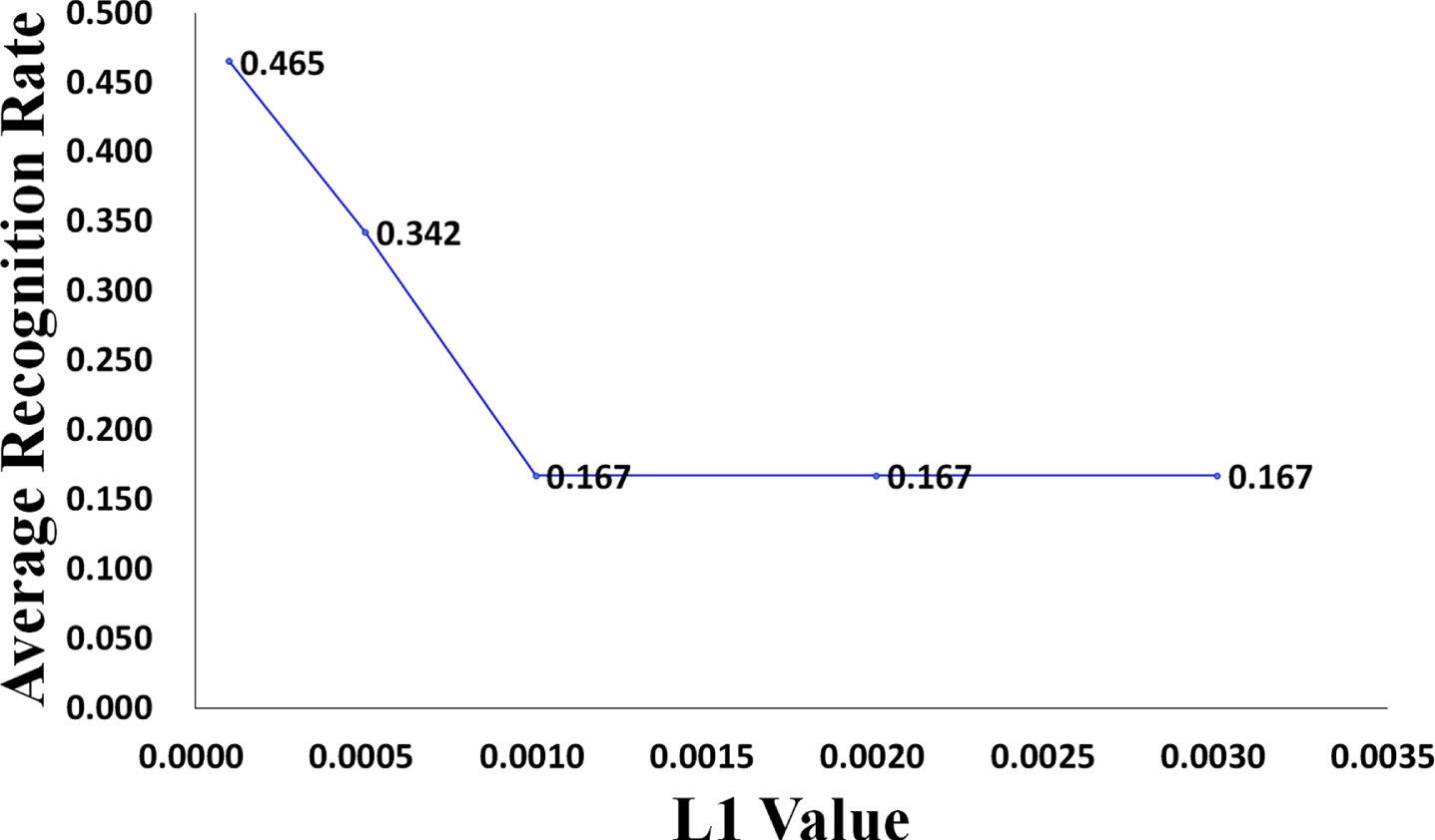
Impact of L1 value on average recognition rate of the TLFF model, where the “Average Recognition Rate” in Fig. 16 refers to the average recognition rate of the six types of wheat (i.e., perfect grains, disease spot grains, moldy grains, sprouted grains, worm-eaten grains, and broken grains).

Fig. 17

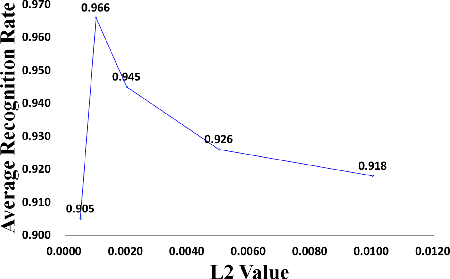
Impact of L2 value on average recognition rate of the TLFF model, where the “Average Recognition Rate” in Fig. 17 refers to the average recognition rate of the six types of wheat (i.e., perfect grains, disease spot grains, moldy grains, sprouted grains, worm-eaten grains, and broken grains).

Experiments show that L2 regularization performs better than L1 regularization in this task. Because, although the L1 regularization method can prevent the model from overfitting to a certain extent, its ability in this respect is not as good as L2 regularization. The wheat dataset we used in this task is not large, so the method with strong ability to prevent the model from overfitting will be more effective.

4.5.3 Activation function

The ReLU activation function can make the SGD optimizer converge faster, however, ReLU suppresses all values less than 0 to 0. In actual operation, if the learning rate is very large, it is likely to cause more neurons in the network to die. The leak parameter in the LeakyReLU activation function is a small constant, and retains some negative values so that not all negative information will be lost.

ReLU and LeakyReLU activation functions have their own advantages. Which activation function we will eventually adopt needs experimental proof. We conduct six experiments on the two types of activation functions to verify which activation function is best for our model. Figure 18 shows the effect of ReLU and LeakyReLU activation functions on the average recognition rate of TLFF. When using the LeakyReLU activation function, the average recognition rate of six experiments is 93.4%. When using the ReLU activation function, the average of six experiments is 96.6%. Therefore, we finally choose the ReLU activation function as the activation function for this task.

Fig.18

Impact of ReLU and LeakyReLU on the average recognition rate of the TLFF model, where the “Average Recognition Rate” in Fig. 18 refers to the average recognition rate of the six types of wheat (i.e., perfect grains, disease spot grains, moldy grains, sprouted grains, worm-eaten grains, and broken grains).

Experiments show that ReLU performs better in this task. Because ReLU is an unsaturated function, it can solve the gradient vanishing problem well. In addition, ReLU can also speed up the convergence of the model.

4.5.4 Optimizer

We compare the gradient descent optimizer SGD with the Adam optimizer using an adaptive learning rate optimization algorithm. The SGD optimizer has the advantages of supporting online updates and easily jumping out of the local optimal solution. The Adam optimizer has the advantages of efficient calculation and simple parameter adjustment. In this task, we compare the effects of two optimizers on the average recognition rate of the TLFF model. We conduct six experiments for each optimizer. Figure 19 shows the impact of Adam and SGD optimizers on the average recognition rate of TLFF. The average recognition rate of the TLFF model when using the SGD optimizer is 96.5%, and is 92.9% when using the Adam optimizer. Experiments show that the performance of TLFF model using SGD optimizer is better than using Adam optimizer. Therefore, we use SGD as the optimizer of the TLFF model in this task.

Fig. 19

Impact of SGD and Adam optimizers on the average recognition rate of the TLFF model, where the “Average Recognition Rate” in Fig. 19 refers to the average recognition rate of the six types of wheat (i.e., perfect grains, disease spot grains, moldy grains, sprouted grains, worm-eaten grains, and broken grains).

Experiments show that the SGD optimizer performs better in this task. The SGD optimizer can automatically escape the relatively poor local optimum. The answer it finally finds is often more general, which makes the generalization performance of the model better.

4.5.5 Learning rate

In order to determine the optimal learning rate in this task, we compare two forms of learning rate, namely, fixed learning rate and decreasing learning rate. Figure 20 shows the impact of fixed learning rate on TLFF model, and the learning rates are shown in Table 18. Figure 21 shows the impact of decreasing learning rate on TLFF model, and the learning rates are shown in Table 19. We decrease the learning rate by one value per iteration of the training set.

Fig.20

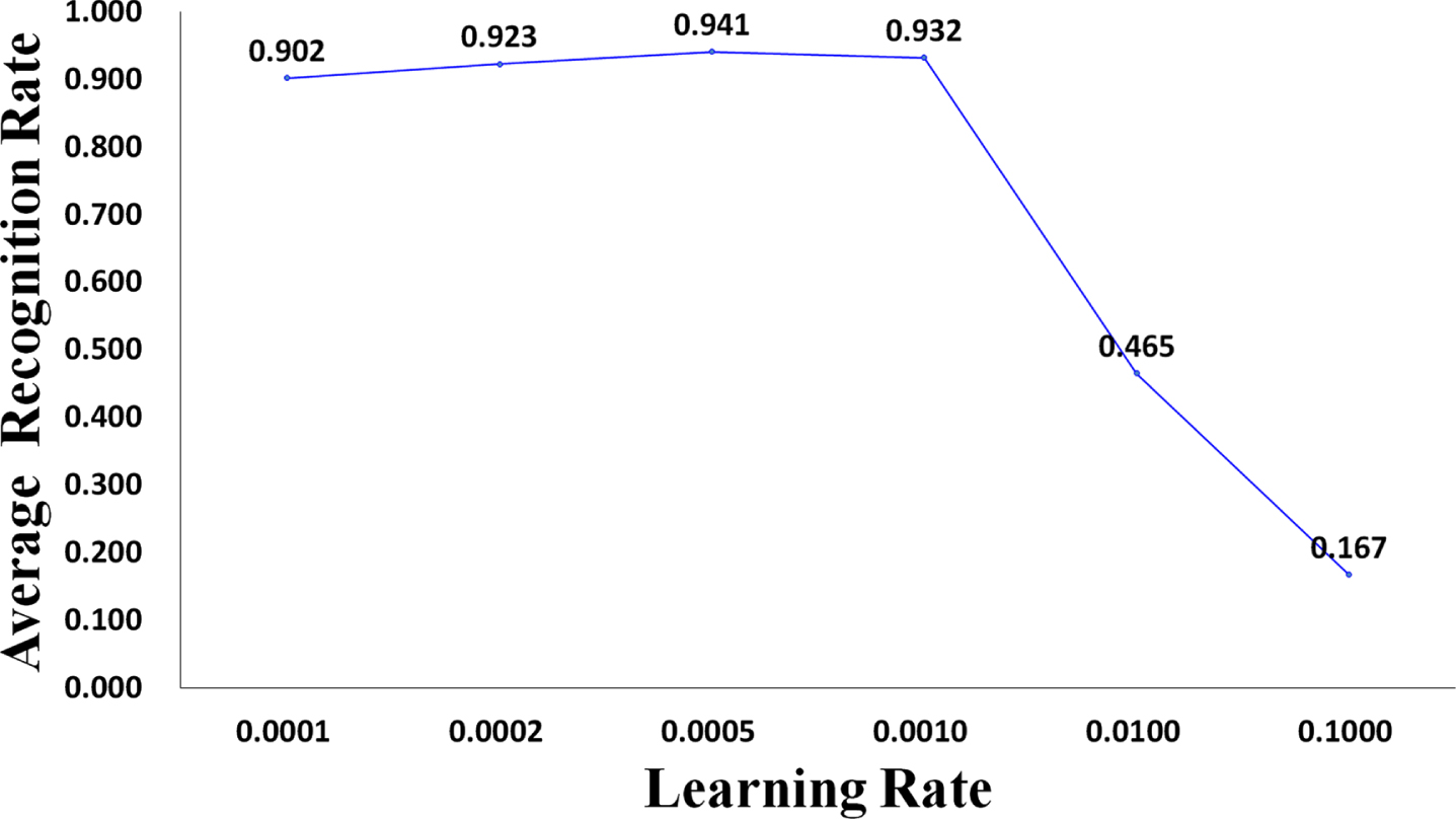
Impact of fixed learning rate on the average recognition rate of the TLFF model, where the “Average Recognition Rate” in Fig. 20 refers to the average recognition rate of the six types of wheat (i.e., perfect grains, disease spot grains, moldy grains, sprouted grains, worm-eaten grains, and broken grains).

Fig. 21

Impact of decreasing learning rate on the average recognition rate of the TLFF model, where the “Average Recognition Rate” in Fig. 21 refers to the average recognition rate of the six types of wheat (i.e., perfect grains, disease spot grains, moldy grains, sprouted grains, worm-eaten grains, and broken grains).

Experiments show that the method of decreasing learning rate has better effect than using fixed learning rate. A learning rate that is too small will reduce the optimization speed of the model, thereby increasing the training time. A too large learning rate will easily cause the model to oscillate in the process of searching for the best advantage, and it is not easy to converge. The decreasing learning rate method can take into account the training efficiency and the stability of the model in the later stage of training.

Table 18

Six cases of fixed learning rate

Cases	Learning rate
1	0.0001
2	0.0002
3	0.0005
4	0.0010
5	0.0100
6	0.1000

Table 19

Five cases of decreasing learning rate

Cases	Initial learning rate	Decrease value
1	0.001	3.03E-5
2	0.0009	2.66E-5
3	0.0008	0.00002
4	0.0007	1.33E-5
5	0.0006	6.66E-6

4.6 Impact of data enhancement

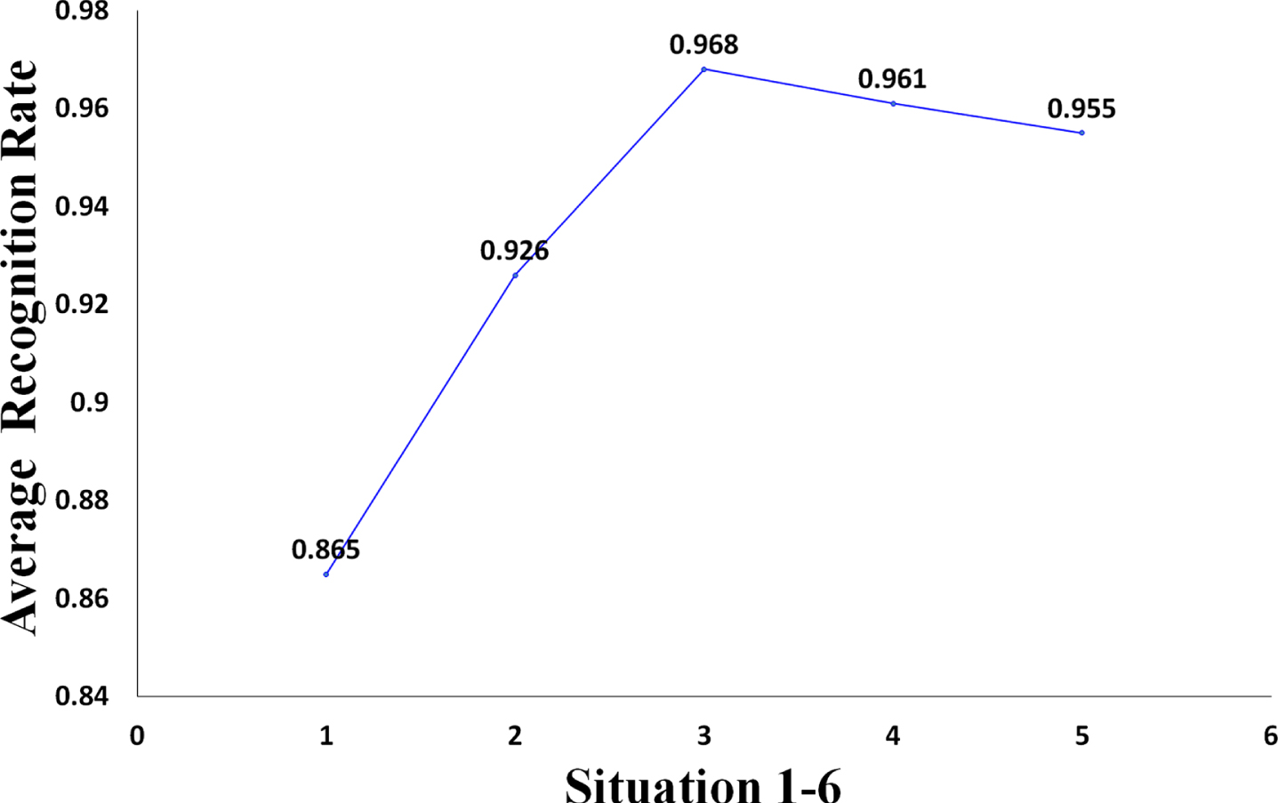
To verify the influence of data enhancement on the model, we conduct two groups of experiments. One group is to input the original wheat images into the TLFF model for training, and obtain the training model of the original images. The other group is to input the data-enhanced images into the TLFF model for training, and obtain the training model of the data-enhanced images. Finally, we test these two groups of training models on the test set. The recognition rate of the two groups of models is shown in Fig. 22. The average recognition rate of the original image model is 91.0%, and the average recognition rate of the data augmentation model is 96.1%. It can be seen that data enhancement can improve the generalization ability of the model.

Fig. 22

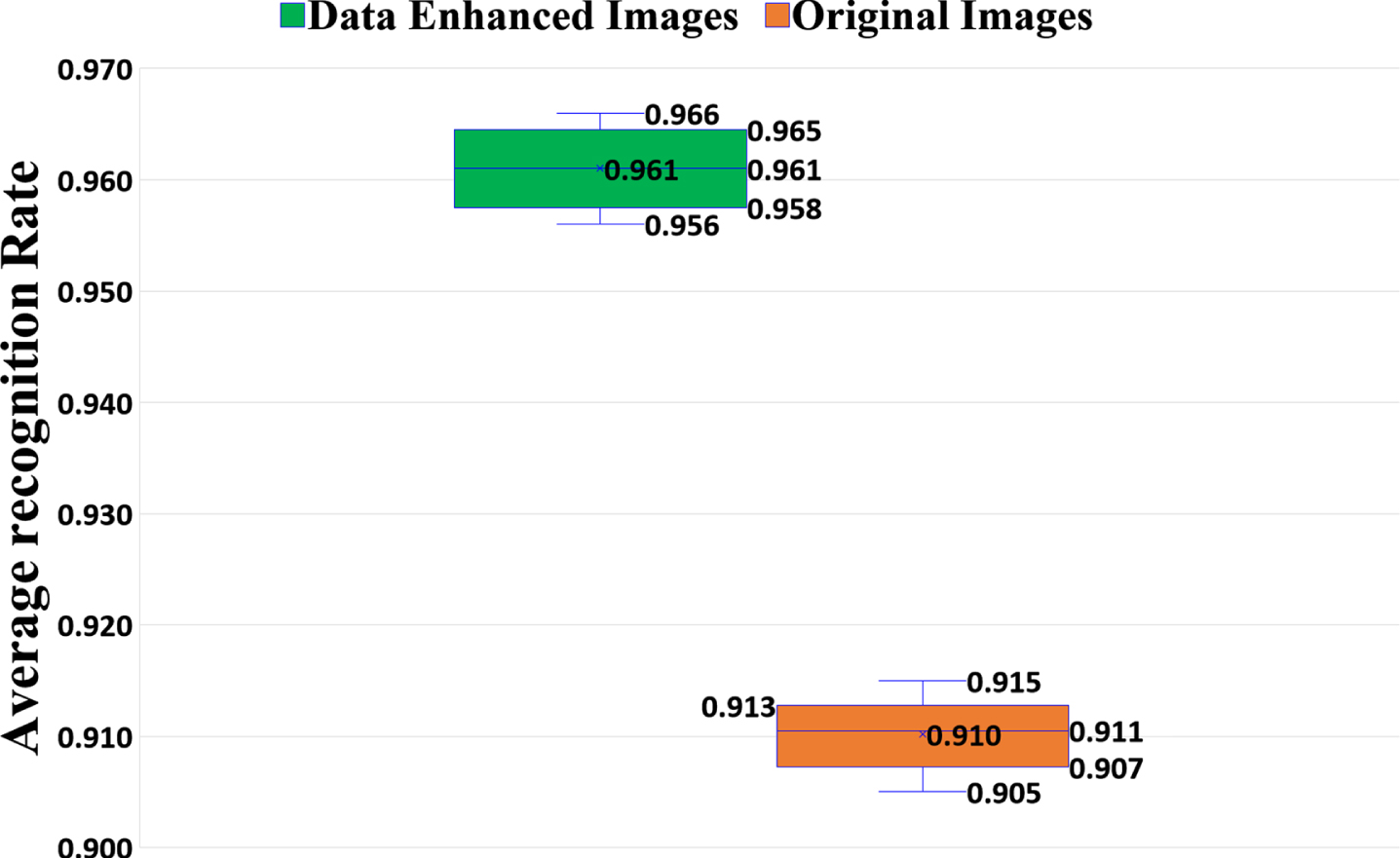
Impact of data enhancement on the average recognition rate of the TLFF model, where the “Average Recognition Rate” in Fig. 22 refers to the average recognition rate of the six types of wheat (i.e., perfect grains, disease spot grains, moldy grains, sprouted grains, worm-eaten grains, and broken grains).

Experiments show that the data enhancement method can significantly improve the performance of the model. In this task, we expand the 12000 training set images to 24000 images through the data enhancement method. On the one hand, data enhancement can increase the amount of data in the training set, thereby improving the generalization ability of the model. On the other hand, data enhancement introduces noise into the training set, which enhances the robustness of the model.

4.7 Statistical analysis of improved results

Before using a method, we decide whether to adopt it or not based on its performance in previous works. In terms of parameter selection, we choose the parameter value that perform well in previous works as the initial value of the parameter in this task. Then it is optimized by parameter adjustment experiments. Parameter adjustment experiments are carried out with the recognition rate as the standard, and the parameter value with the highest recognition rate is selected. We make a total of 7 improvements: model, Dropout, regularization, activation function, optimizer, learning rate, and data enhancement. We conduct 131 experiments and record the results of each experiment. The improvement effect of the model is shown in Fig. 23 and Table 20.

Fig. 23

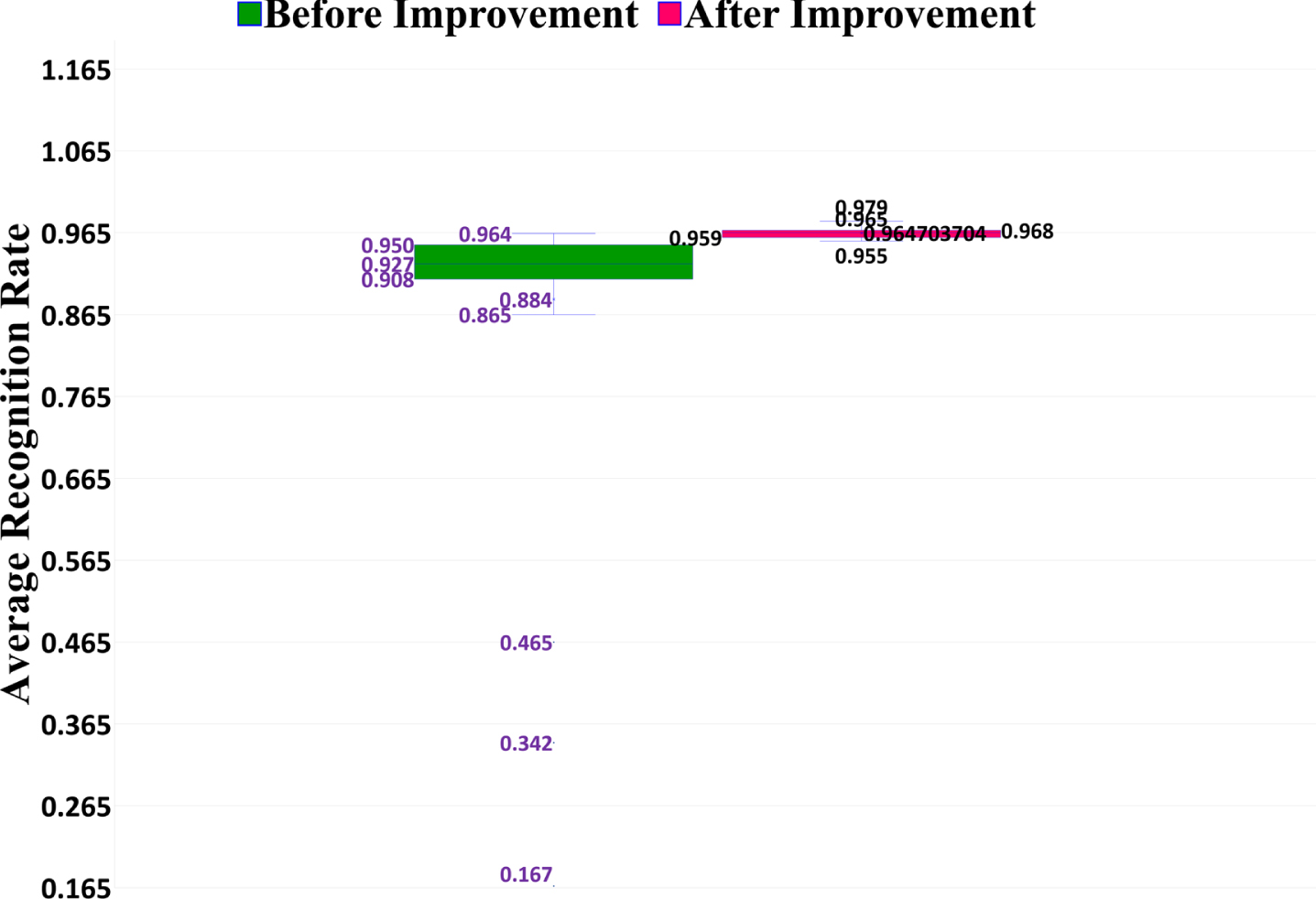
Comparison of recognition results before and after improvement, where the “Average Recognition Rate” in Fig. 23 refers to the average recognition rate of the six types of wheat (i.e., perfect grains, disease spot grains, moldy grains, sprouted grains, worm-eaten grains, and broken grains).

Table 20

Sensitivity analysis results of TLFF model

Parameters	Dropout ratio	Regularization	Activation function	Optimizer	Learning rate
Sensitivity	0.0735	0.8271	0.0644	0.0706	0.8275

It can be seen from Fig. 23 and Table 20 that the average value of the recognition rate after the improvement is 8.1% higher than the average value before the improvement. In addition, the difference between the minimum and maximum values of the improved recognition rate is 2.4%, indicating that after the improvement, the performance of the model is more stable. Experiments show that the improvement measures we take can effectively improve the model performance.

4.8 Sensitivity analysis

We conduct sensitivity analysis on the model to explore the impact of input parameters on the model output. In this section, sensitivity analysis is carried out through the influence of Dropout, regularization, activation function, optimizer, and learning rate on the recognition rate of TLFF model. The specific method is to change each input variable and test various values of the variable, and then introduce the test values of the input variable into the model. We record the maximum and minimum values of the output and calculate the difference between the maximum and minimum values. The ratio of the difference to the maximum output is the sensitivity of the input variable, and the results are shown in Table 21.

Table 21
Comparison of recognition results before and after improvement

Cases Minimum /% Maximum /% Average /%

Before Improvement 16.7 96.4 88.4

After Improvement 95.5 97.9 96.5

Cases	Minimum /%	Maximum /%	Average /%
Before Improvement	16.7	96.4	88.4
After Improvement	95.5	97.9	96.5

It can be seen from Table 21 that learning rate is the most influential parameter for TLFF model recognition rate, followed by regularization, and activation function has the least influence. It can be seen that it is correct to select parameters through comparative experiments, and appropriate parameters can make the model have good generalization performance.

5 Conclusions and future work

We propose a TLFF model based on transfer learning and feature fusion. We use the pre-trained model on the public dataset as the wheat feature extractor and then perform feature fusion and voting to unsound wheat kernel recognition. We use three pre-trained models to fuse by feature concatenating, and then select three best-performing fusion models to vote on their results to achieve the purpose of further improving the recognition rate. The F1 value of the TLFF model is improved by 4.91% compared to the baseline optimal model. We introduce the idea of transfer learning to effectively solve the problem of unsatisfactory recognition rate caused by the small dataset of unsound wheat kernel recognition. Aiming at the problem that the features extracted by a single model are not comprehensive, we effectively solve the problem by feature fusion method. In order to further improve the recognition effect, we introduce the voting mechanism in ensemble learning, so that the recognition result can be effectively improved.

The significance of this study includes three aspects. (1) We propose the Transfer Learning Feature Fusion (TLFF) model, which adopts a transfer learning method that has not been used in the existing unsound wheat kernel recognition tasks. (2) We use multiple models for feature fusion, which effectively improves the quality of wheat feature information. (3) We introduce the voting mechanism in ensemble learning into the recognition task of unsound wheat kernels. The variance is reduced by the ensemble of multiple models, thereby improving the robustness of the model.

Although this model has achieved good results, it also has shortcomings. (1) The model is complex. The complexity of the model will lead to an increase in the number of parameters, which increases the space and time complexity of the model. (2) There are few model categories for fusion. Although the TLFF model uses a three-model fusion method, there are only two types of models, VGG-16 and VGG-19. Few types of fusion models will affect the richness of fusion feature information, resulting in unsatisfactory recognition rate. (3) The model does not perform well in environments with very high real-time requirements, and performs well in environments with high operability requirements. The large scale of the model will affect its real-time performance to a certain extent. The performance of the TLFF model has been significantly improved through transfer learning, feature fusion, and ensemble learning. So there is no need to improve the recognition rate through complex image preprocessing, and it has good operability.

In our future work, we will improve our current work in the following two aspects. (1) For the complex problem of the TLFF model, we will try a lighter network structure on the premise of ensuring the recognition effect. (2) For the problem that the voting optimization algorithm leads to a long model prediction time, we will try other more time-saving algorithms.

Footnotes

Acknowledgments

This work was supported by the Open Project of the Key Laboratory of Food Information Processing and Control of Ministry of Education (KFJJ-2020-109), the National Natural Science Foundation of China (62073123), and Key scientific research projects of higher education institutions in Henan Province (21A520008).

References

Wang

, Wang

, Wen

and Guo

, General situation of world wheat production and processing industry development, Grain Processing 33(4) (2008), 11–12+18.

, Wu

, Chen

, Li

and Wang

, Identification method of unsound kernel wheat based on hyperspectral and convolution neural network, Journal of Electronic Measurement and Instrumentation 31(8) (2017), 1297–1303.

Zhao

, Liu

, He

and Wang

, Analysis on Unsound Grain Composition of Wheat, Journal of Anhui Agricultural Sciences 44(15) (2016), 44–47.

Sladojevic

, Arsenovic

, Anderla

, Culibrk

and Stefanovic

, Deep Neural Networks Based Recognition of Plant Diseases by Leaf Image Classification, Computational Intelligence and Neuroscience(6) (2016), 1–11.

Salman

, Jalal

, Shafait

, Mian

, Shortis

, Seager

and Harvey

, Fish species classification in unconstrained underwater environments based on deep learning, Limnology and Oceanography, Methods 14(9) (2016), 570–585.

, Ren

and Tan

, Fuzzy feature fusion and multimodal degradation prognosis for mechanical components, Journal of Intelligent & Fuzzy Systems 34(6) (2018), 3523–3533.

Shi

, Tondi

, Li

and Barni

, Cnn-based steganalysis and parametric adversarial embedding:a game-theoretic framework, Signal Processing: Image Communication 89(2) (2020), 115992.

Lin

C.-H.

and Wang

T.-Y.

, A novel convolutional neural network architecture of multispectral remote sensing images for automatic material classication, Signal Processing: Image Communication 97(105) (2021), 116329.

D’Acunto

, Martinelli

and Moroni

, From human mesenchymal stromal cells to osteosarcoma cells classification by deep learning, Journal of Intelligent & Fuzzy Systems 37(6) (2019), 7199–7206.

10.

Zhu

, Zhang

, Qi

and Lu

, Vision-based defects detection for bridges using transfer learning and convolutional neural networks, Structure and Infrastructure Engineering 16(7) (2020), 1037–1049.

11.

Wang

, Li

, Wang

and Xu

, Histopathological imageclassification based on cross-domain deep transferred featurefusion, Biomedical Signal Processing and Control 68(2021), 102705.

12.

Zhang

, Yan

and Wang

, Quality-guided lane detection bydeeply modeling sophisticated traffc context, SignalProcessing: Image Communication 84(7) (2020), 115811.

13.

Fadl

, Han

and Li

, CNN spatiotemporal features and fusion for surveillance video forgery detection, Signal Processing: Image Communication 90 (2021), 116066.

14.

Hou

, Zhao

, Hu

and Liu

, No-reference video quality evaluation by a deep transfer CNN architecture, Signal Processing: Image Communication 83(1) (2020), 115782.

15.

, Zhang

and Wu

, Automatic grape leaf diseases identication via unitedmodel based on multiple convolutional neural networks, Information Processing in Agriculture 7(3) (2020), 418–426.

16.

, Ji

and Deng

, Automatic detection and severityassessment of pepper bacterial spot disease via multimodels based onconvolutional neural networks, International Journal ofAgricultural and Environmental Information Systems 11(2) (2020), 29–43.

17.

, Shao

, Wang

and Han

, Recognition of Corn Leaf Spotand Rust Based on Transfer Learning with Convolutional NeuralNetwork, Transactions of the Chinese Society for AgriculturalMachinery 51(02) (2020), 230–236+253.

18.

, Liao

, Zhang

, Yu

, Wang

, Gao

and Wang

, Image Recognition of Maize Disease Based on Asymmetric Convolutional Attention Residual Network and Transfer Learning, Science Technology and Engineering 21(15) (2021), 6249–6256.

19.

Long

, Ouyang

, Liu

and Fu

, Image recognition of Camellia oleifera diseases based on convolutional neural network & transfer learning, Transactions of the Chinese Society of Agricultural Engineering 34(18) (2018), 194–201.

20.

Wang

, Zhang

, Liu

and Zhang

, Image classification of tomato leaf diseases based on transfer learning, Journal of China Agricultural University 24(6) (2019), 124–130.

21.

Yang

, Tang

and Cao

, Research on Small Sample Image Recognition Based on Transfer Learning, Journal of Physics: Conference Series 1302(3) (2019), 032039.

22.

Singh

and Om

, Newborn face recognition using deep convolutional neural network, Multimedia Tools and Applications 76(18) (2017), 19005–19015.

23.

Song

, Wang

Collaborative deep networks for pedestrian detection, in: 2017 IEEE Third International Conference on Multimedia Big Data (BigMM) 2017, pp. 146–153.

24.

Polishetty

, Roopaei

, Rad

A next-generation secure cloud-based deep learning license plate recognition for smart cities, in: 2016 15th IEEE International Conference on Machine Learning and Applications (ICMLA), 2016, pp. 286–293.

25.

Guo

and Ding

, A hybrid deep learning cnn-elm model and its application in handwritten numeral recognition, Journal of Computational Information Systems 11(7) (2015), 2673–2680.

26.

Jiang

, Shen

, Feng

and Yu

, An optimized cnn-based quality assessment model for screen content image, Signal Processing: Image Communication 94(4) (2021), 116181.

27.

Krishna

B.V.

, Pandey

A.K.

and Siva

A.P.

, Kumar, Universally domain adaptive algorithm for sentiment classication using transfer learning approach, International Journal of System Assurance Engineering and Management 12 (2021), 542–552.

28.

Zhai

, Liu

and Song

, Staging Diagnosis of Liver Fibrosis Based on Transfer Learning Strategy, Electronic Science and Technology 34(06) (2021), 11–16.

29.

Deng

, Wang

, Tang

, Huang

and Zhu

, A deep transfer learning method based on stacked autoencoder for cross-domain fault diagnosis, Applied Mathematics and Computation 408 (2021), 126318.

30.

and Meng

, Pedestrian detection method based on multi-scale feature fusion, Microcomputer Applications 37(06) (2021), 117–120+124.

31.

Liu

, Qian

, Li

, Wang

and Zhang

, CAFFNet: Channel Attention and Feature Fusion Network for Multi-target Traffic Sign Detection, International Journal of Pattern Recognition and Artificial Intelligence 35(07) (2021).

32.

, Dou

, Song

and Yang

, Insulator Nondestructive TestingBased on Feature Fusion CNN, Electronic Science and Technology 34(07) (2021), 26–30.

33.

Heintz

and Doherty

, A knowledge processing middleware framework and its relation to the JDL data fusion model, Journal of Intelligent & Fuzzy Systems 17(4) (2006), 335–351.

34.

Liu

, Feng

and Xue

, Fault diagnosis of hydraulic retraction system based on multi-source signals feature fusion and health assessment for the actuator, Journal of Intelligent & Fuzzy Systems 34(6) (2018), 3635–3649.

35.

, Zhang

, Ren

and Sun

, Spatial Pyramid Pooling in Deep Convolutional Networks for Visual Recognition, IEEE Transactions on Pattern Analysis and Machine Intelligence 37(9) (2015), 1904–1916.

36.

Pan

S.J.

and Yang

, A survey on transfer learning, IEEE Transactions on Knowledge and Data Engineering 22(10) (2010), 1345–1359.

37.

Luo

, Jayas

D.S.

and Symons

S.J.

, Comparison of statistical and neural network methods for classifying cereal grains using machine vision, Transactions of the ASAE 42(2) (1999), 413–419.

38.

Singh

C.B.

, Jayas

D.S.

, Paliwal

and White

N.D.G.

, Identication of insect-damaged wheat kernels using short-wave near-infrared hyperspectral and digital colour imaging, Computers and Electronics in Agriculture 73(2) (2010), 118–125.

39.

Chen

Real-time Detection of Kernel-like Impurity and Unsound Kernel in Wheat Using Machine Vsion, Ph.D. Dissertation, Zhejiang University, 2012.

40.

Neethirajan

, Jayas

D.S.

and White

N.D.G.

, Detection of sprouted wheat kernels using soft x-ray image analysis, Journal of Food Engineering 81(3) (2007), 509–513.

41.

Zhang

, Chen

, Zhou

, Wang

and Wu

, and H.Wang, Identification of unsound kernels in wheat based on image processing and neural network, Science and Technology of Cereals, Oils and Foods 22(03) (2014), 59–63.

42.

Zhu

Study on wheat appearance quality inspection based on machine vision, M.S. Dissertation, Jiangsu University, 2021.

43.

Hao

, Qing

, He

and Li

, Recognition of unsound wheat kernels based on hyperspectral fusion image, Modern Computer (36) (2019), 44–48.

44.

, Zhou

, Wang

, Wu

and Liu

, Hyperspectral Detection of Unsound Kernels of Wheat Based on Convolutional Neural Network, Food Science 38(24) (2017), 283–287.

45.

Dong

, Wu

, Liu

, Mao

and Zhang

, Research on hyperspectral image detection method of wheat unsound kernel, Journal of Electronic Measurement and Instrumentation 31(7) (2017), 1074–1080.

46.

Liu

Research on Unsound Kernel of Wheat Recognition Based on Hyperspectral Imaging, M.S. Dissertation, North China University of Water Resources and Electric Power, 2021.

47.

Liu

, Wang

, An

, Wei

and Luo

, X. Chen and Y. Yan,Study on Detection Method of Wheat Unsound Kernel Based onNear-Infrared Hyperspectral Imaging Technology, Spectroscopyand Spectral Analysis 39(1) (2019), 223–229.

48.

Zhu

, Zhuo

, Huang

and Li

, Wheat grain integrity image detection system based on cnn, Transactions of the Chinese Society for Agricultural Machinery 51(05) (2020), 36–42.

49.

Zhang

, Wang

, Wu

and Zhu

, Research on imperfect wheat grain recognition based on Python-OpenCV image processing technology, Journal of Henan University of Technology (Natural Science Edition) 42(6) (2021), 105–112.

50.

, Wu

, He

, Hu

and Qing

, Imperfect wheat kernel recognition combined with image enhancement and conventional neural network, Journal of Computer Applications 41(3) (2021), 911–916.

51.

Cao

, He

, Dong

, Shi

and Xiong

, Identification of Unsound Kernels in Wheat Based on CNN Deep Model, Modern Computer(36) (2017), 9–14.

52.

Zhang

Machine vision inseption of wheat apprearance quality based on deep learning, master Thesis, M.S. Dis sertation, Northwest Agriculture and Forestry Technology University, 2019.

53.

Almadhor

, Rauf

H.T.

, Lali

M.I.U.

, Damasevicius

, Alouffifi

and Alharbi

, AI-Driven Framework for Recognition of Guava Plant Diseases through Machine Learning from DSLR Camera Sensor Based High Resolution Imagery, Sensors 21(11) (2021), 3830.

54.

Abayomi-Alli

O.O.

, Damaeviius

, Misra

and Maskeliunas

, Cassava disease recognition from low-quality images using enhanced data augmentation model and deep learning, Expert Systems 38(4) (2021), 12746.

55.

Oyewola

D.O.

, Dada

E.G.

, Misra

and Damasevicius

, Detecting cassava mosaic disease using a deep residual convolutional neural network with distinct block processing, PeerJ Computer science 7(2) (2021), e352.

56.

Kundu

, Rani

, Dhaka

V.S.

, Gupta

, Nayak

S.C.

, Verma

, Ijaz

M.F.

and Wozniak

, IoT and Interpretable Machine Learning Based Framework for Disease Prediction in Pearl Millet, Sensors 21(16) (2021), 5386.

57.

, Fang

, Li

and Zheng

, Tomato leaf disease detection based on deep feature fusion of convolutional neural network, China Sciencepaper 16(07) (2021), 701–707.

58.

, Tao

, Fang

, Zheng

, Wang

and Jin

, Identifying Anthracnose and Black Spot of Pear Leaves on Near-infrared Hyperspectroscopy, Transactions of the Chinese Society for Agricultural Machinery 53(2) (2022), 221–230.

59.

, Qiao

and Rao

, Recognition of grape leaf diseases and mobile application based on transfer learning, Transactions of the Chinese Society of Agricultural Engineering 37(10) (2021), 127–134.

60.

Wang

, Zhang

, Yao

, Yang

, Zhang

and Fan

, Disease identification and spot detection of potato leaves based on convolutional neural network, Journal of Chinese Agricultural Mechanization 42(11) (2021), 122–129.

61.

Bao

, Huang

, Hu

and Liang

, Identification of maize leaf diseases using improved convolutional neural network, Transactions of the Chinese Society of Agricultural Engineering 37(06) (2021), 160–167.

62.

Liu

and Gao

, Identification of multiple leaf diseases using improved SqueezeNet model, Transactions of the Chinese Society of Agricultural Engineering 37(02) (2021), 187–195.

63.

Xiang

, Zhai

, Huang

and Liu

, Plant disease identification based on Xception-CEMs neural network, Journal of Chinese Agricultural Mechanization 42(08) (2021), 177–186.

64.

Shi

, Xiao

, Huang

, Hu

and Zhang

, Research on recognition of silkworm diseases based on Convolutional Neural Network, Journal of Chinese Agricultural Mechanization 43(1) (2022), 150–157.

65.

Yue

, Li

, Zhao

and Wang

, Crop Disease Image Recognition Based on Improved VGG Network, Journal of Agricultural Mechanization Research 44(6) (2022), 18–24.

66.

Zhu

, Wang

, Ren

and Tao

, Fruit Tree Leaf Disease Recognition Based on Residual Network and Multi Feature Fusion, Forest Engineering 38(1) (2022), 108–114+123.

67.

Huang

, Bi

, Mo

, Qin

, Lin

and Wan

, Image Recognition Method of Citrus Diseases and Pests Based on Multi-scale Feature Fusion, Radio Engineering 52(3) (2022), 407–416.

68.

Fan

, Zhou

, Xu

and Peng

, Corn Disease Recognition under Complicated Background Based on Improved Convolutional Neural Network, Transactions of the Chinese Society for Agricultural Machinery 52(3) (2021), 210–217.

69.

Krizhevsky

, Sutskever

and Hinton

G.E.

, ImageNet classificationwith deep convolutional neural networks, Communications of theACM 60(6) (2017), 84–90.

70.

Srivastava

, Hinton

, Krizhevsky

, Sutskever

and Salakhutdinov

, Dropout: A simple way to prevent neural networks from overfitting, The Journal of Machine Learning Research 15(1) (2014), 1929–1958.

71.

Ruan

Digital Image Processing, Tsinghua University Press, 2009, pp. 155–159.

Unsound wheat kernel recognition based on deep convolutional neural network transfer learning and feature fusion

Abstract

Keywords

1 Introduction

2 Related work

2.1 Methods for unsound wheat kernel recognition

2.1.1 Unsound wheat kernel recognition based on artificial extraction features

2.1.2 Unsound wheat kernel recognition based on hyperspectral image

2.1.3 Unsound wheat kernel recognition based on deep learning

2.2 The latest researches on plant disease recognition

2.3 Problems with existing methods and motivation for this study

3.3 Feature fusion

Table 3 The case of fusion model 1 Model VGG-16 VGG-16 VGG-19 Output (None, 7, (None, 7, (None, 7, shape 7, 512) 7, 512) 7, 512) Fusion shape (None, 7, 7, 1536)

4.1 Experimental settings

4.1.1 Dataset

4.2.1 TLFF model data

Table 7 Parameter quantity and distribution of VGG-16+VGG-16+VGG-19 model Layer Number of parameters VGG-16 Model 14714688 VGG-16 Model 14714688 VGG-19 Model 20024384

4.4 Model selection

4.4.1 Single transfer learning model

4.5 Influence of parameters

4.5.1 Dropout ratio

Table 21 Comparison of recognition results before and after improvement Cases Minimum /% Maximum /% Average /% Before Improvement 16.7 96.4 88.4 After Improvement 95.5 97.9 96.5

Footnotes

Acknowledgments

References

Table 3
The case of fusion model 1

Model VGG-16 VGG-16 VGG-19

Output (None, 7, (None, 7, (None, 7,

shape 7, 512) 7, 512) 7, 512)

Fusion shape (None, 7, 7, 1536)

Table 7
Parameter quantity and distribution of VGG-16+VGG-16+VGG-19 model

Layer Number of parameters

VGG-16 Model 14714688

VGG-16 Model 14714688

VGG-19 Model 20024384

Table 21
Comparison of recognition results before and after improvement

Cases Minimum /% Maximum /% Average /%

Before Improvement 16.7 96.4 88.4

After Improvement 95.5 97.9 96.5