
Abstract
In Intelligent Transport Systems (ITS), vision is the primary mode of perception. However, vehicle images captured by low-cost traffic cameras under challenging weather conditions often suffer from poor resolution and insufficient detail representation. On the other hand, vehicle noise provides complementary auditory features that offer advantages such as environmental adaptability and a large recognition distance. To address these limitations and enhance the accuracy of low-quality traffic surveillance classification and identification, an effective audio-visual feature fusion method is crucial. This paper presents a research study that establishes an Urban Road Vehicle Audio-visual (URVAV) dataset specifically designed for low-quality images and noise recorded in complex weather conditions. For low-quality vehicle image classification, the paper proposes a simple Convolutional Neural Network (CNN)-based model called Low-quality Vehicle Images Net (LVINet). Additionally, to further enhance classification accuracy, a spatial channel attention-based audio-visual feature fusion method is introduced. This method converts one-dimensional acoustic features into a two-dimensional audio Mel-spectrogram, allowing for the fusion of auditory and visual features. By leveraging the high correlation between these features, the representation of vehicle characteristics is effectively enhanced. Experimental results demonstrate that LVINet achieves a classification accuracy of 93.62% with reduced parameter count compared to existing CNN models. Furthermore, the proposed audio-visual feature fusion method improves classification accuracy by 7.02% and 4.33% when compared to using single audio or visual features alone, respectively.
Introduction
In Intelligent Transport Systems (ITS), effectively classifying and identifying vehicles using the collected vehicle information is a crucial yet challenging task. Traditional methods for vehicle classification involve extracting vehicle features through machine learning techniques like Histogram of Orientation Gradients (HOG) [9, 15] and Scale-invariant Feature Transform [16, 32], and then inputting these features into classifiers such as Support Vector Machines (SVM) and iterative processes for classification. The continuous advancements in image processing and pattern recognition have greatly influenced the field of vehicle classification and detection [4, 18]. Traffic monitoring techniques can generally be classified into two categories: invasive sensor-based approaches [1, 33] and non-invasive sensor-based approaches, depending on the type of sensors employed. Non-intrusive sensors are typically positioned above or beside the road and encompass various types, including road surveillance systems, Unmanned Aerial Systems, microphone sensors, among others. In comparison to invasive sensors, non-intrusive ones provide ample vehicle information such as vehicle geometry and path of travel. Furthermore, their monitoring data is less affected by road conditions, and they are relatively straightforward to install and maintain [11].
Road surveillance represents the quintessential application of ITS. To capture high frame rates and achieve superior image quality, road surveillance typically adopts highly precise cameras equipped with glare suppression capabilities. However, due to economic constraints in developing countries, substantial investments in high-precision ITS applications and deployments are often unattainable. Consequently, low-cost traffic surveillance cameras are commonly employed in such regions, albeit at the expense of image quality [17]. These cameras, offering lower signal-to-noise ratios, present several challenges such as diminished image resolution, compromised color reproduction, and inadequate representation of details [12]. Moreover, the classification and recognition of vehicle features become increasingly complex and arduous, given the diverse range of vehicles with variations in shape, color, and logos.
Efforts have been made to tackle the issue of poor-quality vehicle images, which lack essential information and suffer from the inability to capture intricate details. Wang et al. [31] devised a methodology involving the sequential usage of three blur kernels and random exposure to generate low-quality vehicle images. They further designed a hybrid objective function to facilitate image detail recovery and employed Generative Adversarial Networks (GANs) to transform blurred images into high-resolution counterparts for subsequent classification. Meanwhile, Tas et al. [25] proposed a lightweight Convolutional Neural Network (CNN) model based on an enhanced VGG architecture, achieving an impressive accuracy rate of 92.9% when evaluated on a dataset comprising tiny (100×100 pixels) and low-resolution (96 dpi) vehicle surveillance images. Zivkovic et al. [21] adopted a simple CNN framwork consisting of three convolutional layers and three pooling layers. Instead of a fully connected layer, they utilized an efficient Extreme Gradient Boosting classifier to classify the extracted features. Furthermore, Tao et al. [23] addressed the challenge by utilizing small convolutional kernel sizes to suppress noise and retain details in low-quality vehicle images, particularly those captured under nighttime conditions. Notably, the issue becomes more pronounced when photographing vehicles traveling at high speeds, resulting in motion blur effects that are especially apparent in images of smaller vehicles and diminish the availability of visually discernible information.
Audio information has the potential to complement visual features [27]. Employing acoustic sensors to measure noise levels before and after a vehicle passes by can be an economical approach that provides essential data for vehicle classification. However, it requires high-quality data acquisition. Moreover, unlike visual images, acoustic sensors installed on the roadside are unaffected by visual obstructions, as well as light and weather conditions [5]. In their work, Wang et al. [3] enhanced the spectral properties of the Mel-spectrogram by applying a discrete cosine transform, resulting in the calculation of improved Mel Frequency Cepstrum Coefficient (MFCC) features for vehicle detection. Abesser et al. [10], on the other hand, utilized Mel-spectrograms and inter-correlation features of vehicle audio signals as inputs to various convolutional neural networks, enabling the prediction of car, truck, and motorcycle classes, as well as the estimation of their direction of motion.
Audio-visual feature fusion is a technique that leverages the interaction between visual and audio information to enhance the effectiveness of tasks such as audio-visual classification and recognition. By extracting and combining effective vehicle audio-visual features from audio and video data, it becomes possible to achieve more accurate and robust vehicle classification and recognition [20]. Initially, eigenvectors from different modalities reside in separate subspaces, creating heterogeneous gaps [29]. To improve decision output accuracy, it is beneficial to narrow down the segmentation gap of the joint semantic subspace while maintaining semantic integrity. This involves integrating correlations between different modal features and adopting a unified approach for modeling and classifying both image features of vehicles and vehicle audio features. Piyush et al. [22] utilized audio information by identifying peaks in the smoothed short-time energy of audio signals. They collected video features around these peak locations through background subtraction and three-frame difference techniques, which were then fed into a multilayer feed-forward artificial neural network for classification. Selbes and Sert [2] extracted MFCC and visual features from video signals and fused them using a join operator. To address environmental changes like occlusion and motion blur that can affect vehicle classification accuracy, Wang et al. [27] employed visual reconstruction. They extracted vehicle geometric, local structural, and auditory features, combining them to achieve optimal classification accuracy by fusing geometric, HOG, and MFCC features. Other studies have explored feature fusion using self-encoders [7], GAN [34], spatial pyramids [30], and fuzzy genetic algorithms [28].
In summary, traditional machine learning methods rely on hand-designed algorithms to extract features and suitable classification methods. On the other hand, CNN training benefits from larger datasets, more parameters, expressive model features, reduced subjectivity in testing methods, and better performance on large-scale datasets. Regarding the extraction of audio signal features in vehicle fusion techniques, previous researchers primarily extracted one-dimensional MFCC features or audio waveforms. However, Mel-spectrograms, which are two-dimensional RGB color images, can serve as inputs to CNNs. Mel-spectrograms capture detailed variations in both time and space, providing a comprehensive and richer description of the data. Their scale mimics the non-linear perception of sound by the human ear, emphasizing greater discrimination at lower frequencies. This makes Mel-spectrograms more suitable as auditory features in audio-visual fusion technology for vehicles.
The main contributions of this paper are as follows: An Urban road vehicle audio-visual (URVAV) dataset with highly aligned audio-visual features was created, containing low-quality vehicle images as well as the corresponding vehicle audio files. A model Low-quality Vehicle Images Net (LVINet) for low-quality vehicle image classification is proposed and compared with the well-known CNN model and good accuracy is obtained with a reduced number of parameters. The proposed methods for the fusion of audio-visual features of vehicles are compared and achieve better performance than single-feature classification.
The subsequent sections of the paper are structured as follows: Section 2 delineates the procedure employed to construct the URVAV dataset, encompassing information on data volume, along with the dataset preprocessing methodology. Section 3 expounds upon the model architectures employed in this study, encompassing visual, auditory, and audio-visual feature integration. Section 4 elucidates the specifics of the experiments conducted and presents the corresponding validation outcomes. Finally, conclusions are drawn and future research directions are proposed in Section 5.
Urban road vehicle audio-visual (URVAV) dataset
Acquisition of data
One of the primary obstacles when utilizing multimodal data for mobile vehicle classification is the scarcity of tagged data. In a real-world vehicle driving environment, uncontrollable factors such as visual obstructions and disruptive noises exist. Thus, acquiring vehicle movement data, aligning audio-visual information, and tagging the data pose significant challenges. To address these challenges, audio and video information of vehicles from various road scenarios were collected for the dataset while minimizing external interference to the greatest extent possible.
The initial data collection was conducted using audio-visual sensors installed on the roadside. The video footage of vehicle movement was recorded using an Olympus E-P5 device, while the sound signal of vehicle movement was captured using an AWA6228 Avionics sound level meter. Figure 1 illustrates one of the multiple collection locations, showcasing the specific coordinates of the data collection site on a satellite map, the environment in which data was collected, and a schematic representation of the collection process. The collection location was situated in the middle section of the road, offering sufficient length for most vehicles to complete their acceleration phase. Simultaneous audio and video recordings were made to facilitate the subsequent data processing steps, including cropping, sorting, and labeling.

Environment and schematic diagram for data collection.
Prior to commencement of the data acquisition process, it is permissible for the acquisition device to capture both the visual motion and auditory sound associated with clapping hands. By carefully examining the video timeline and analyzing the audio waveform, the parameters related to delay or synchronization of the device can be adjusted to ensure a proper alignment of the acquired audio-visual data. Furthermore, it is of utmost importance to exercise caution in safeguarding the confidentiality and privacy of the data during the acquisition phase. Overall, an extensive amount of more than 80 hours was dedicated to collecting audio and video data to create the URVAV dataset. Challenges encountered during the acquisition process, such as excessive background noise, visual obstruction, and overlapping audio interference, necessitated a meticulous manual screening and filtering procedure to identify valid data samples that would yield satisfactory recognition outcomes.
A video clip of two seconds each before and after the vehicle passes through the video recording equipment (total length of 4 seconds) is intercepted from the video to ensure that there is no visual occlusion of the video vehicle. An audio clip, also of 4 seconds duration, corresponding to the video clip was intercepted, and the available audio files were filtered so that each audio sample contained only the noise of one vehicle passing the acoustic sensor.Ultimately, a total of 2195 audio-visual samples were chosen and categorized, with an equal distribution of half the samples encompassing rainy, foggy, and dark conditions. Regarding vehicle classification, five distinct vehicle types, namely Car, Large truck, Light truck, SUV, and Van, were chosen for identification research based on their frequency of occurrence within the collected dataset. The quantity of sample files is displayed in Table 1. The URVAV dataset lends itself to the application of vehicle classification and recognition utilizing audio, video, or multimodal features. Various configurations of visual and auditory signals contribute to the evaluation of technological capabilities and facilitate the design of intelligent systems.
Vehicle category labels and numbers
Specific details regarding the dataset cannot be divulged currently, given the confidentiality agreements in place. A plethora of devices equipped with the capacity to capture audio-visual data exist, and should one adhere to the aforementioned methodology for data acquisition and labeling, it would be feasible to undertake comparable or more extensive research endeavors by dedicating considerable time and effort.
The front-side view of each vehicle is intercepted from the video clip in frames and the image size is modified to 50×50 pixels with a resolution of 96 dpi.After the recorded video is processed, an example of the front-side view of the five types of vehicles is shown in Fig. 2.
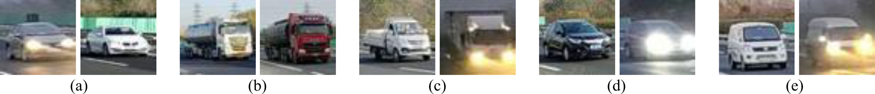
Example of a front-side view of a vehicle. (a) Car. (b) Large truck. (c) Light truck. (d) SUV. (e) Van.
It is saved as a.wav format file with a sampling rate of 44.1 KHz, and the data that meets the audio and video data requirements at the same time is manually labeled to finally form the URVAV dataset. The speech signal is a one-dimensional time domain signal, intuitively difficult to see the pattern of change of frequency, so the speech signal can be converted into a two-dimensional image.
The audio signal x [n] is pre-emphasised to obtain the signal y [n], as shown in Equation (1). The a in the difference equation is the pre-emphasis coefficient, which usually takes a value between 0.9 and 1.0, and was taken to be 0.97 for this experiment.
The speech signal y [n] of length N after pre-emphasis is subjected to windowing and frame-splitting to obtain f [n], as shown in Equation (2). The length of each frame is taken to be wlen, the displacement of the latter frame to the former is expressed as inc, and the overlap between two neighbouring frames is overlap = wlen - inc. Each of the split frames is multiplied by the Hamming window function to increase the continuity at both ends of each frame and reduce spectral leakage.
Next, an N-point Fast Fourier Transform is done on each frame of the signal after the frame-splitting and windowing operations to compute the spectrum f
i
(n), the Fast Fourier Transform is also known as the Short-Time Fourier Transform, where N takes the value of 512 in this study, and n takes an integer between 0 and 512.
The power spectrum p is calculated using Equation (4), and the spectral energy of the speech signal is obtained by taking the mode square of the spectrum f
i
(n) for a speech signal of length N.
Equation (5) shows how the original frequency f and mel frequency f mel are converted. Pass the spectrogram through a mel scale filter bank to obtain a Mel- spectrogram, and the calculation formula of the mel filter bank is shown in Equation (6). A number of band-pass filters H m (k) are set in the spectral range of speech, each filter has triangular filtering characteristics, and its central frequency is f (m), where the range of m is 1 ⩽ m ⩽ M, and M is the number of filters and its value has a magnitude of 24. The bandwidths of these filters are equal over a range of values of frequency.
The Mel-spectrogram obtained by performing the above operations on the labelled audio file is shown in Fig. 3 and has a size of 224×224.
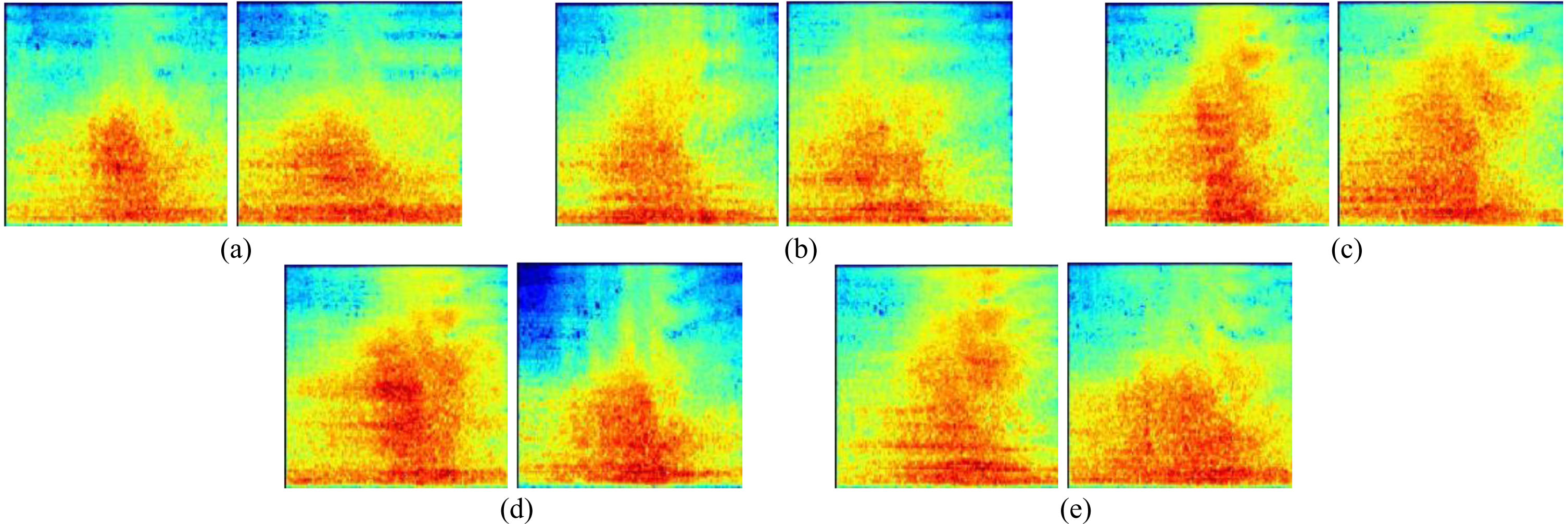
Example of Mel-spectrogram of vehicle noise. (a) Car. (b) Large truck. (c) Light truck. (d) SUV. (e) Van.
Vehicle classification model based on low-quality images
It is first necessary to determine the size and number of channels in the input image and the number of output categories to be predicted. Convolutional layers play a crucial role in CNNs. In this specific case, the low-quality vehicle image is fed through convolutional layers with a kernel size of 3×3. This enables the model to extract local features at different positions within the image. Following each convolutional layer, Rectifier Linear Units (ReLU) and Batch Normalization layers are employed. These additional layers serve to eliminate unwanted noise, accelerate network training and convergence, and regulate the gradient explosion to prevent gradient vanishing [24].
The Fire module of SqueezeNet [6], as depicted in Fig. 4, consists of multiple layers. The first layer is a dimensionally compressed convolutional layer with a kernel size of 1×1. This compression reduces the number of channels to 1/4 of the original count. Subsequently, the outputs are split into two branches: one branch performs a 1×1 convolutional operation, while the other branch conducts a 3×3 convolutional operation. This multi-scale convolution allows for the extraction of different receptive fields, enhancing the model’s ability to capture diverse feature information and improve classification performance. The outputs of these two branches are then concatenated based on their dimensions. It is worth noting that the Fire module plays a more significant role in classifying small-size images.

Structure of the Fire module.
By substituting the 3×3 convolutional kernel in the Fire module with an asymmetric convolution using kernel sizes of 1×3 and 3×1, the computational overhead is reduced to approximately 67% (calculated as (1×3 + 3×1) / (3×3)). This modification leads to a decrease in the number of parameters and overall computational effort required, all while preserving comparable accuracy. In convolutional neural networks, the MaxPool2D layer is responsible for spatial downscaling and feature compression. It decreases the number of parameters and computational resources required by the model while preserving essential information. To construct an optimal LVINet for low-quality vehicle image classification, several adjustments are made. These include tuning the number of convolutional layers (ranging from 1 to 4), configuring hyperparameters such as kernel size and stride, modifying the number (ranging from 1 to 3)and order of the enhanced multi-scale convolutional kernel parallel modules, and fine-tuning the dimensionality of each layer. The resulting feature maps with a size of 7×7 are then fed into a fully-connected layer to predict the most likely classes. The structure of the complete model can be seen in Fig. 5.

Structure of the LVINet.
MobileNet V2 [19] is a network introduced by the Google team in 2018. It offers higher accuracy and a smaller model compared to MobileNet V1, making it suitable for various image classification and detection tasks in mobile applications. Figure 6 illustrates that MobileNet V2 follows an inverted residual structure with linear bottlenecks. This structure takes a low-dimensional compressed representation as input and expands it to higher dimensions. Lightweight deep convolutions are applied in the intermediate extension layers to filter nonlinear features. The features are then projected back to a low-dimensional representation using linear convolutions. The network has a wider shape in the middle and narrower shapes at both ends, resembling a spindle. Shortcut connections are established between narrow bottleneck layers, but only when the stride value is 1 and the input and output feature matrices have the same shape.

Structure of MobileNetV2 network.
Method 1: Feature fusion module for tensor stitching. As shown in Fig. 7, multiple tensors are combined into a single tensor, which represents a method of joining features extracted from different modalities into a single high-dimensional feature vector. This means that the number of features (channels) describing the image itself has increased, but the information under each feature has not. The limitations of this feature fusion approach are the high-dimensional feature vectors generated and the inability to model complex relationships as it straightforwardly fuses two modal features.

Structure of the tensor stitching feature fusion module.
Method 2: The feature fusion module based on weight assignment is shown in Fig. 8. The extracted audiovisual features are stitched together in the channel dimension, and the dimension is changed to 2 by convolutional layers. Using SoftMax to generate corresponding weights of different proportions, the original features are weighted to highlight useful feature information, suppress irrelevant features, and enhance feature representation.

Structure of the weight assignment feature fusion module.
Method 3: Feature fusion module for spatial-chan-nnel attention. To reduce the computational complexity, the audiovisual features F
v
and F
a
of size C×H×W are extracted and reduced in size by 1×1 convolution to obtain the new audiovisual features Fv1 and Fa1. For the spatial feature fusion part of the left half of Fig. 9, the

Structure of the spatial-channel attention feature fusion module.
For the channel feature fusion part in the right half of Fig. 9, a matrix multiplication operation is performed on visual feature Fv1 and
Finally, Fav1 and Fav2 are summed to obtain highly correlated audiovisual features both spatially and channel-wise, which are fed into the classifier for classification.
The vehicle classification and recognition methods presented in this paper are compared to those outlined in prior literature, as depicted in Table 2. LVINet is the CNN model proposed in this paper for classifying lower-quality vehicle images. The conversion of one-dimensional sound signals into two-dimensional Mel-spectrograms, which provide a more comprehensive and detailed description of the data, helps capture important audio features. The audio-visual features are extracted separately by CNN before being fused, which enhances the classification of low-quality vehicle images. The URVAV dataset proposed in this paper has a large amount of data, highly aligned audiovisual features, and contains audiovisual data in complex weather.
Comparative table of related literature
Comparative table of related literature
The parameters of the hardware system used in the next experiments were the CPU of the experimental computer was AMD Ryzen 7 5800 H, the GPU model was NVIDIA GeForce RTX 3060 and the RAM was 32GB. The parameters of the software system are the operating system is Windows 11 64-bit, the experimental software version is PyCharm 2021.3.1, the Python version is 3.9.7, the PyTorch version is 1.11.0, and the Cuda version is 11.3. In the experiments, SGD was chosen as the optimizer, the momentum moment was set to 0.9, the initial learning rate was set to 0.001, the epoch was set to 150,the batch size was set to 32, and URVAV dataset was randomly divided into training, validation, and test sets, with the ratio of training, validation and test sets being 6:2:2.
Evaluation of vehicle classification models for low-quality images
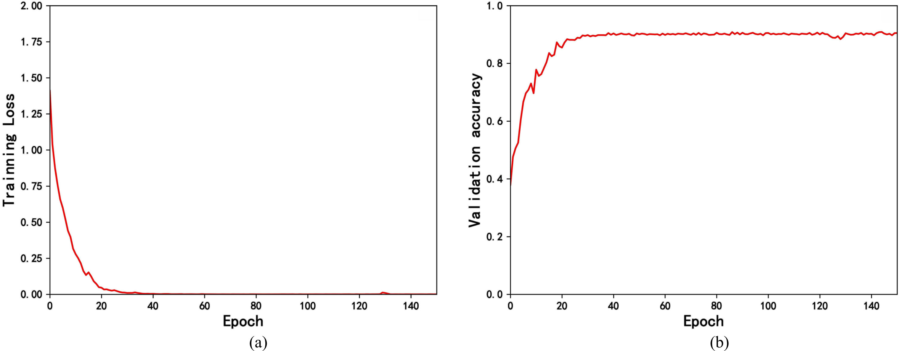
In order to evaluate the classification results of LVINet for low-quality vehicle images, the method proposed in this paper is tested on the URVAV dataset. To improve the generalization and robustness of the training model, three methods of data augmentation are used: horizontal flipping, image saturation change, and image sharpening for low-quality vehicle image datasets. Figure 10(a) shows the training loss curve of the proposed model, with the horizontal axis indicating the number of iterations and the vertical axis indicating the training loss value, which converges rapidly up to 20 epochs, after which it fluctuates slightly and eventually converges to 0 and is stable. Figure 10(b) shows the variation curve of the accuracy of the validation set, with the horizontal axis indicating the number of iterations and the vertical axis indicating the accuracy of the validation set, which reaches a stable value of around 60.

Training curves of LVINet. (a) Training loss curve. (b) Validation set accuracy curve.
The test results of the model were compared with the testing results of VGG16 [17], Resnet18 [11], and Resnet34 [11] in terms of accuracy and complexity. The results in Table 3 show that while VGG16 and Resnet34 provide higher accuracy, the proposed LVINet model trained in this paper yields an acceptable accuracy (93.62%) with a shorter training time and a smaller number of parameters. In practice, when hardware constraints are encountered, accuracy is often sacrificed in an acceptable range to reduce model complexity, so the proposed LVINet can be used as a network model for the classification of low-quality vehicle images.
Comparison of test accuracy and complexity of LVINet and CNN models
In order to evaluate the results of MobileNetV2 classification of vehicles by vehicle noise, the method proposed in this paper is tested on the URVAV dataset. Three methods of data augmentation are used for the Mel-spectrograms generated from vehicle noise: adding white noise, changing the image saturation, and time-frequency domain masking. Figure 11(a) shows the training loss curve of the proposed model, where the horizontal axis indicates the number of iterations and the vertical axis indicates the training loss value. Figure 11(b) shows the accuracy curve of the validation set, where the horizontal axis indicates the number of iterations and the vertical axis indicates the accuracy of the validation set, with the training loss and validation accuracy reaching stability at the 40th round. The ambient noise in the surroundings can hinder the clarity of the sound signal, thus augmenting the challenge associated with classifying vehicles solely based on auditory cues. Consequently, the classification accuracy derived from a single auditory feature tends to be slightly lower compared to that obtained from a single visual feature.
Training curve of MobileNetV2. (a) Training loss curve. (b) Validation set accuracy curve.
In the next experiments, the three feature fusion approaches proposed in this paper were tested on the URVAV dataset to verify the superiority of multimodal feature fusion in the vehicle classification task. As depicted in Fig. 12, the five curves correspond to LVINet, MobileNet V2, and the proposed three vehicle audio-visual feature fusion methods. By contrasting the training curves of vehicle classification and recognition using single visual and auditory features with those obtained through feature fusion, the following trends are observed from the figure. In Fig. 12(a), the vertical axis represents the training loss value. Notably, due to the amalgamation of auditory features with visual features, the trained features manifest heightened complexity, resulting in an inevitable increase in parameter count. Consequently, the training loss curve of the fusion model converges around the 50th epoch. However, in Fig. 12(b), it is evident that the validation set accuracy curves for the three vehicle audio-visual feature fusion methods outperform those of single visual and auditory features for vehicle classification. Notably, the spatial-channel attention-based feature fusion method (fusion method 3) stands out with its validation set accuracy curves beginning to converge around the 50th epoch. This remarkable performance underscores the model’s ability to acquire more generalized features during training, effectively avoiding overfitting. Moreover, the model exhibits strong adaptability to the audiovisual data in the URVAV dataset, indicating excellent generalization capabilities.

Comparison of training curves. (a) Comparison of training loss curves. (b) Comparison of validation set accuracy curves.
In Fig. 13, the confusion matrix for the spatial- channel based feature fusion structure test set is depicted. Each row in the matrix represents the predicted category, each column represents the true category, and the diagonal line indicates the number of correctly predicted samples. The graph shows that most of the misclassifications are between “SUV” and “Car", because they not only have a similar front appearance, but also have similar engine noise. In addition, the highest prediction accuracy is for the Van and Large truck. Table 4 presents the accuracy, recall, precision, and F1 scores of various network models on the URVAV test set. The implementation of the spatial channel-based audio-visual feature fusion architecture yields a substantial enhancement in vehicle classification accuracy. Specifically, there is an improvement of 7.02% and 4.33% compared to the single visual and auditory features, respectively, resulting in an impressive accuracy of 97.95%. The remaining evaluation metrics also exhibit notable improvements.
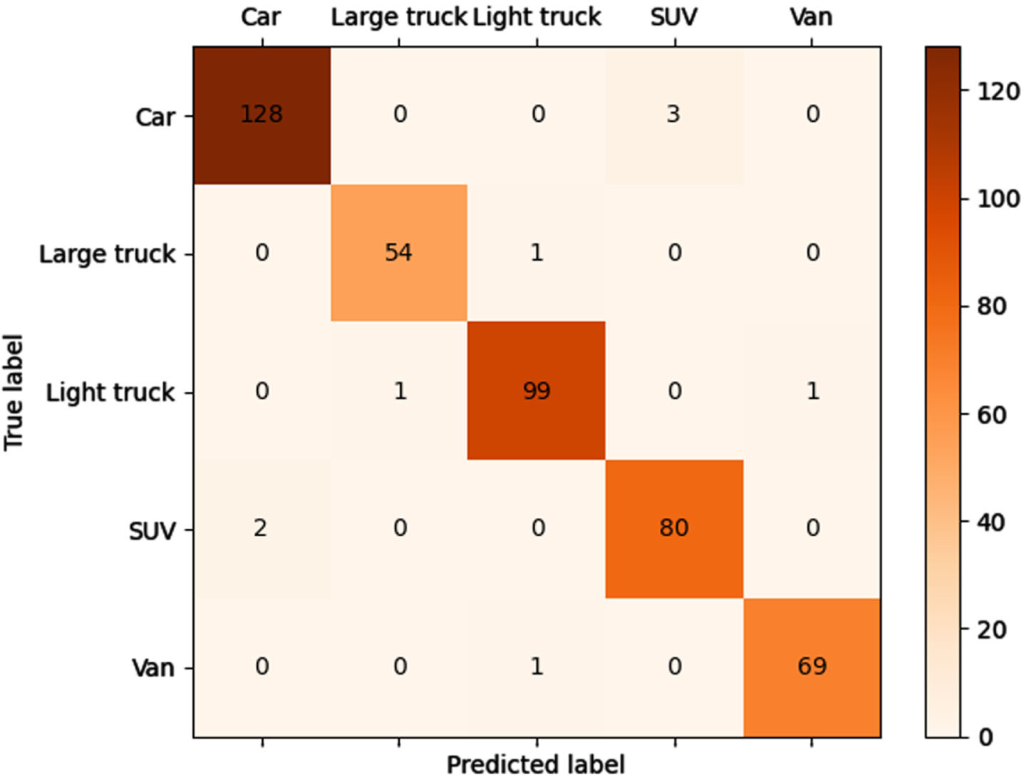
Confusion matrix of feature fusion structure based on spatial channel attention.
Performance metrics of different network models on the test set
Figure 14 shows the comparison of recall, precision, and F1 scores for different network models on the URVAV test set. From Fig. 14(a) and Fig. 14(b) it can be seen that the category of SUVs with poor prediction accuracy showed a significant increase in recall and precision (on average about 10%), while the other four categories also showed a significant increase in recall and precision. The F1 score in Fig. 14(c) considers both the accuracy and recall of the classification model, can be seen as a weighted average of the model accuracy and recall, and can be seen to be better for vehicle classification using audio-visual feature fusion based on spatial channel attention. Figure 14 and Table 4 show that the model proposed in this paper can accurately classify low-quality vehicle data through the audio-visual features of vehicles in challenging external environments such as different weather conditions and vehicle ambiguities.

Comparison of recall, precision and F1 scores of different network models after testing on URVAV dataset (a) Recall (b) Accuracy (c) F1 scores.
The purpose of this paper is to achieve accurate classification of low-quality vehicle images and demonstrate the superiority of audio-visual feature fusion in vehicle classification. To accomplish this, the paper establishes the URVAV dataset, which consists of 2,195 audio-visual samples with five vehicle types collected under complex weather and lighting conditions. The paper proposes a CNN model called LVINet specifically designed for classifying low-quality vehicle images. The model focuses on categorizing low-quality front-side view images of vehicles with dimensions of 50×50 and a resolution of 96 dpi. It is then compared to a well-known CNN model. The results show that LVINet achieves an impressive accuracy rate of 93.62% on the test set, while also reducing computational requirements. Furthermore, the paper compares three different vehicles audio-visual feature fusion approaches that highlight semantically relevant feature information and suppress irrelevant features. Among them, the spatial-channel-attention-based approach demonstrates its superiority on the URVAV dataset, achieving a test set accuracy of 97.95%. This showcases the effectiveness of incorporating spatial channel attention in enhancing the discriminative power of fused features.
It is worth noting that the experimental scenarios considered in this study were limited, and the URVAV dataset only collected single-vehicle movements. In real-world large-scale urban traffic scenarios, multiple vehicles pass through data collection equipment simultaneously, which requires preprocessing of the collected audio and video data. Future research aims to improve the generalizability of the methodology by diversifying datasets and exploring novel data preprocessing techniques. Ad ditionally, optimizing the model and deploying it on hardware devices, such as embedded systems or dedicated chips, can enable real-time vehicle recognition and classification.
Footnotes
Acknowledgments
This work was supported in part by the Tianjin Science and Technology Program, China (Grant No. 21YDTPJC00050), and the Foundation Project of the Science and Technology on National Key Laboratory of Electromagnetic Space Security (Grant No. 2021JCJQLB055008).