Improved noise-filtering algorithm for AdaBoost using the inter-and intra-class variability of imbalanced datasets

Abstract

Boosting methods are known to increase performance outcomes by using multiple learners connected sequentially. In particular, Adaptive boosting (AdaBoost) has been widely used owing to its comparatively improved predictive results for hard-to-learn samples based on misclassification costs. Each weak learner minimizes the expected risk by assigning high misclassification costs to suspect samples. The performance of AdaBoost depends on the distribution of noise samples because the algorithm tends to overfit noisy samples. Various studies have been conducted to address the noise sensitivity issue. Noise-filtering methods used in AdaBoost remove samples defined as noise based on the degree of misclassification to prevent overfitting to noisy samples. However, if the difference in the classification difficulty between classes is considerable, it is easy for samples from classes that are difficult to classify to be defined as noise. This situation is common with imbalanced datasets and can adversely affect performance outcomes. To solve this problem, this study proposes a new noise detection algorithm for AdaBoost that considers differences in the classification difficulty of classes and the characteristics of iteratively recalculated sample weight distributions. Experimental results on ten imbalanced datasets with various degrees of imbalanced ratios demonstrate that the proposed method defines noisy samples properly and improves the overall performance of AdaBoost.

Keywords

AdaBoost noise-robust learning noise-filtering class imbalance class separation

1 Introduction

Boosting methods are known to obtain improved predictive results by sequentially combining multiple learners that are interconnected [1]. In particular, adaptive boosting (AdaBoost) has shown improved performance on hard-to-learn samples given its use of adaptive learning [2 –5]. An individual learner focuses on suspect samples that are frequently misclassified. This can lead to adaptation to hard-to-learn samples. However, AdaBoost has a critical drawback in that it tends to overfit noisy samples. Base learners treat noisy samples as more important than hard-to-learn samples because noisy samples are misclassified continuously regardless of the progress of adaptive learning, which increases the weights of noisy samples [6 –8]. Noisy samples with an excessively large weights degrades the performance of base learners, which in turn corrupt the performance of the ensemble model [8].

Many studies have sought to improve AdaBoost to make it more robust to noise. Algorithm-level methods have been designed to decrease the degree of adaptivity over suspect samples using a robust loss function or with an updating scheme [9, 10]. Data-level methods limit the effect of noisy samples for future learning after detecting them based on recalculated sample weights or margins representing the tendencies found in previous learning sessions [11 –13]. Data-level approaches can be divided according to whether or not noisy samples are preserved. The noise-filtering method removes them for future boosting rounds by setting the sample weight to zero [11 , 14], but the noise-correcting approach preserves them by either decreasing the sample weight or changing the labels of noisy samples [6 , 15–17].

Noise-filtering methods are commonly used because the process of implementation and tuning the parameters is simple compared to algorithm-level methods [18 –20]. However, noise-filtering methods not only clean the data, but can also result in information loss due to discriminating excessive samples, including informative samples, as noise [14, 21]. This problem is particularly important when dealing with imbalanced data, where the numbers of samples of certain classes are significantly higher than the numbers of other types. Classification with imbalanced data is a serious problem because learners tend to be biased toward the majority class 1 . Even if the minority samples are ignored, low errors are achievable such that it becomes easy to induce learning bias towards majority classes, which implies better prediction performance in the minority class.

AdaBoost is a cost-sensitive learning method that solves this problem by preventing base learners from becoming biased to the majority class. Usually, minority samples are assigned high sample weights owing to the high frequency of misclassifications, causing base learners to focus on minority samples rather than majority samples. However, adaptivity to minority samples of AdaBoost tends to degrade the classification performance, as minority samples tend to be eliminated at an excessive rate [9, 22]. Ignoring the stronger tendency toward misclassification of the minority class causes this problem.

To address this issue, in this paper we propose a new AdaBoost algorithm with an improved noise-filtering algorithm that considers that classification difficulties differ depending on the class in imbalanced data.

The remainder of this paper is organized as follows. A brief review of noise-filtering methods used in AdaBoost is provided in Section 2. The proposed method is explained in detail in Section 3. The experimental procedures and results are presented in Section 4. The conclusions and future work are provided in Section 5.

2 Related work

Many methods have been the goal of decreasing the degree of noise sensitivity in AdaBoost algorithms. The importance weight for each sample can increase rapidly, as it is calculated using the exponential loss function. As mentioned in Section 1, these methods are divided into two types: (1) algorithm-level and (2) data-level methods. The methodologies in the algorithm-level approach intend to decrease the degree of adaptivity over suspect samples by using either a robust loss function or an updating scheme. This approach is expected to increase the importance weight smoothly by using robust loss functions. Accordingly, alternative functions such as the logistic function mathematically demonstrated as smooth [8], the normalized sigmoid cost function [23] and the nonconvex function [24] are used. In addition, methods to regularize the distribution of the sample weights have been proposed. Noisy samples still tend to be assigned relatively high sample weight values, though it could be better to limit the contribution of a specific sample for training. These methods are divided into two types: those that set bounded ranges [25, 26] and those that prevent skewness of the sample weights [27, 28].

Data-level methods intend to limit the contribution for the training of noisy samples that are detected considering certain trends during classification, such as sample weights and margins that are updated sequentially. One of the simplest ways to limit the influence of noise is to eliminate it, and this is done using a noise-filtering method. Noise-filtering methods remove noisy samples by setting their importance weights to zero. Two typical methods that use sample weights to detect noise are ORBoost [11] and RUSBoostWO [13]. They use a common noise-filtering framework; however, one difference is that RUSBoostWO applies a noise-filtering method to a balanced dataset obtained by random undersampling [29]. The noisy samples are defined when the value of the sample weight exceeds than threshold, d. This is defined as follows:

$w_{t + 1} (i) = {\begin{matrix} 0, & if w_{t + 1} (i) \geq d \\ w_{t + 1} (i), & otherwise \end{matrix}$ (1) where w_t (i) is the sample weight of the i-th sample at iteration t. The threshold d is computed by multiplying the mean of the sample weights and a constant, as follows: $d = μ_{t} \cdot C,$ (2) where μ_t refers to the mean of the sample weight w_t+1 (i) at iteration t, and C is a user-defined constant. Disregarding cases that exceed the threshold is necessary to improve the classification performance because adapting to a few samples with abnormally high importance weights cannot improve the performance any more.

Noise-correcting methods repair noisy samples either by penalizing the sample weights or swapping the labels to minimize the loss [6 , 15–17]. Noise-correcting methods that use the margins to detect noisy samples, as typical noise-correcting methods, define noisy samples after sufficient results are collected and require additional information, such as the neighborhood for noise detection. The margin of each sample is calculated according to the weighted average of the predictions of the individual classifiers. This is done as follows:

$m_{i} = y_{i} \sum_{t = 1}^{T^{*}} α_{t} h_{t} (x_{i}),$ (3) where m_i refers to the margin of the i-th sample x_i with label y_i (y_i ∈ {-1, 1}) using the results until T^* iterations (T^* ≤ T and T is the number of weak learners in the final boosting model). The range of m_i is from -1 to 1 because the value of y_i is either -1 or 1. In addition, α_t and h_t (x_i) represent the weight of the base learner and the predicted label at the iteration t, respectively. In contrast to the methods using sample weights, a noisy sample is defined when the value of the margin is lower than the threshold, m_L. The low margin value indicates that it is difficult to correctly classify the corresponding sample. Generally, samples with the negative margin values are defined as noise. In other words, the weights of samples considering the margin are defined as follows:

$w_{T^{*} + 1} (i) = {\begin{matrix} 0, & if m_{i} < m_{L} \\ w_{T^{*} + 1} (i), & otherwise \end{matrix}$ (4) Even though the margin is useful to find noisy samples, both noisy and informative samples tend to have a negative margin; therefore, numerous informative minority samples can be eliminated. Hence, the improved methods while using the margin have been proposed to consider the characteristics of noisy samples. It is known that noisy samples are prone to exist in the opposite class area and can thus tend to be surrounded by opposite samples. In other words, the improved methods select noisy samples from samples with negative margins using additional information or processes. In one study [12], Hoeffding’s inequality was used to measure the abnormality of the value of the margin. EAdaBoost defined the representative vector of each sample considering the margins and sample weights, and then applied the weighted k-NN rule to distinguish noisy samples [30]. In [31], only a specified number of samples with negative margin values was defined as noise by sorting the margins in ascending order.

However, noise-filtering is typically faster than noise correction because noisy samples are removed once they are defined as containing noise. It is also necessary to tune only the parameters associated with noise detection [18 –20], whereas noise-correcting methods are necessary properly to correct noisy samples after noise detection, as noisy samples are continuously used for learning. In summary, the strengths of noise-filtering methods are usability and simplicity.

However, noise-filtering methods have several drawbacks. First, an excessive number of samples can be removed unless the number of noisy samples is bounded [32 –35], which decreases the performance [21]. Second, informative samples could be defined as noisy [14]. These two problems are particularly critical for imbalanced data, as informative minority samples are likely to be removed. The elimination of informative minority samples is highly detrimental to the classification performance outcome [22]. Usually, boosting methods focus on samples that are misclassified frequently. For imbalanced data, minority samples tend to be misclassified frequently; therefore, excessively biased learning for the majority can be prevented. However, when the noise-filtering method is applied, minority samples are prone to be defined as containing noise. If the classification complexity differs for each class, which is frequently observed when handling imbalanced data, previous noise-filtering methods for AdaBoost are not appropriate for detecting noisy samples. When using these methods, a large number of minority samples are prone to be defined as noise, and removing minority informative samples may be as harmful as reserving minority samples containing noise. To address this problem, in this paper, an improved noise-filtering algorithm for AdaBoost is proposed to define noisy samples properly by considering differences when classifying different classes.

3 Proposed Method

This study proposes a new noise-filtering method using the sample weights of AdaBoost for imbalanced data. The key point of the proposed noise-filtering method is to set different thresholds to detect noisy samples for each class. The first method (called Case 1) to obtain the thresholds utilizes the mean of the sample weights for each class, similar to ORBoost and RUSBoostWO. However, the mean may not be sufficient to represent the characteristics of the distribution of the sample weights because it does not consider deviation and skewness in the distributions. Therefore, this study additionally proposes a second method to set the thresholds considering the distribution of the sample weights for each class using a boxplot (called Case 2).

3.1 Case 1

The threshold value for noise detection is greatly affected by the classification complexity of the majority class in the case of imbalanced data. Considering that the minority class is more difficult to correctly classify than the majority class [36], many minority samples can have much higher sample weights than the threshold value. Figure 1 shows this problematic tendency with Abalone data as an example. In this figure, the boxplots show the distribution of the sample weights depending on the number of iterations, and the red line refers to the threshold values at each iteration. In addition, the green line represents the ratio of the noisy samples for each class at each iteration. As shown in Figure 1, the proportion of samples defined as noisy increased rapidly as the learning progressed.

Fig. 1

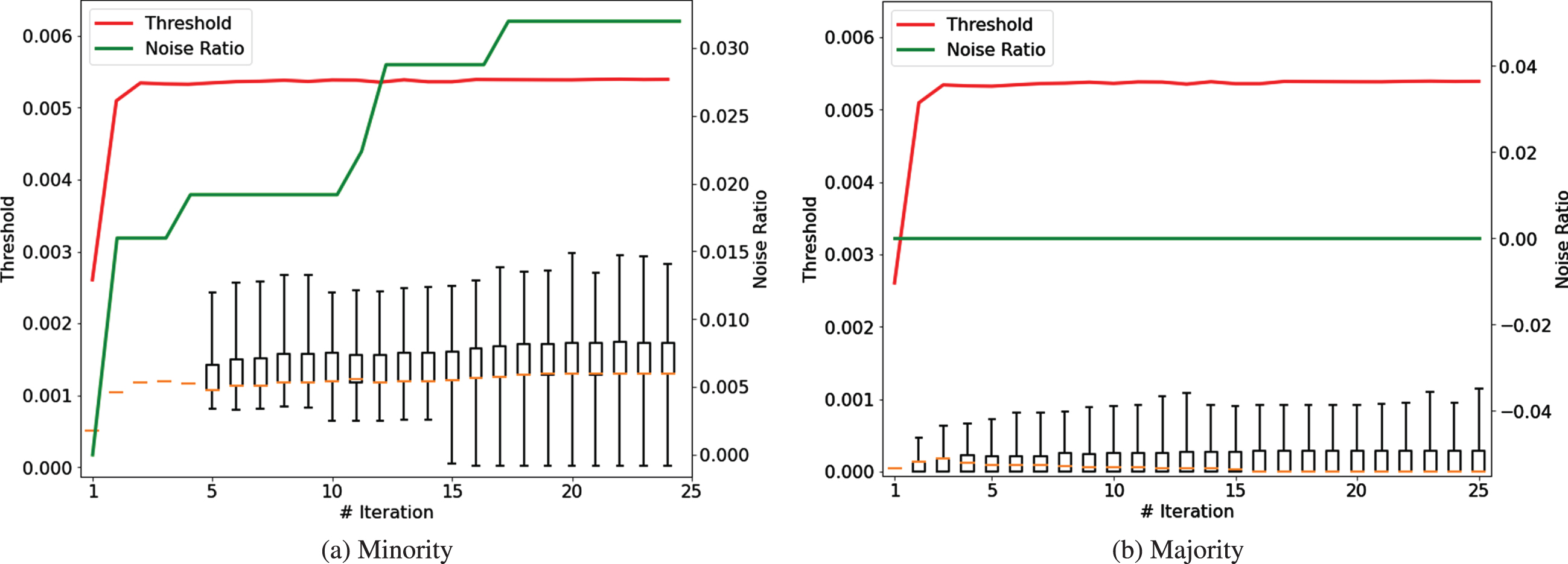
Distributions of sample weights, thresholds for noise detection, and the proportions of noise samples for the majority and minority classes

Unless noise-filtering methods are applied separately to each class, an excessively large number of minority samples can be defined as noise owing to the relatively high classification difficulty compared to the majority class. To solve this problem, the threshold to define noise should be set differently for each class. Case 1 sets different threshold values depending on class while continuing to use the same approach to obtain the thresholds of ORBoost and RUSBoostWO. The threshold values of Case 1 are defined as follows:

$\begin{matrix} d_{t, n}^{1} = μ_{t, n} \cdot α \\ d_{t, p}^{1} = μ_{t, p} \cdot α \end{matrix}$ (5) where $d_{t, p}^{1}$ and $d_{t, n}^{1}$ represent the threshold values for the minority and majority classes, respectively, and μ_t,p and μ_t,n correspondingly represent the average of sample weights at iteration t for the minority and majority classes, respectively. In addition, α is a user-defined parameter identical to C in Eq. (2). The superscript 1 represents Case 1. The value of the threshold for the minority class is higher than that of the majority class because minority samples are frequently misclassified.

3.2 Case 2

To consider not only the centrality of the distributions of the sample weights but also other characteristics of the distributions, such as deviation and skewness, the second approach to obtain the thresholds utilizes a boxplot. A boxplot is commonly used to depict the distribution of data graphically using quartiles [37]. In a boxplot, a box represents the centrality range, and fences represent the upper and lower limits. Typically, they are defined through quartiles to divide the data, ordering the dataset in an ascending order into quarters. The interquartile range (IQR) is defined between the first quartile (Q₁) and the third quartile (Q₃) to depict the box. The two fences, the lower fence (f_L) and the upper fence (f_U), are defined as follows:

$\begin{matrix} f_{L} = Q_{1} - β \cdot IQR \\ f_{U} = Q_{3} + β \cdot IQR \end{matrix}$ (6) where β is a user-defined constant. Both the lower and upper fences use IQR such that the distances from the box are identical for the fences. In other words, these fences do not consider the skewness of the distributions. However, when data are skewed, many points can exceed the fences and are often erroneously classified as outliers [38]. Moreover, the sample weights of AdaBoost for a dataset with noise show a right-skewed distribution, which is well illustrated by the box plots in Figure 1.

To consider the skewness of the distributions of the sample weights for noise-filtering, Case 2 uses an adjusted boxplot for skewed data. In many studies related to improved boxplots, the degree of skewness is calculated based on two sub-elements [38 –41]; semi-interquartile-range from upper quartile (SIQR_U) and semi-interquartile-range from lower quartile (SIQR_L) that are split at the median, where SIQR represents the semi-interquartile range. SIQR_U and SIQR_L are defined as follows:

$\begin{matrix} {SIQR}_{U} & = Q_{3} - Q_{2} \\ {SIQR}_{L} & = Q_{2} - Q_{1} \end{matrix}$ (7)

Using SIQR_U and SIQR_L, the adjusted boxplots for skewed data generally use a longer distance from the box when setting the fences compared to that in the ordinary boxplot. One typical method is to use Bowley’s coefficient(B_c) [39], which is defined as follows:

$\begin{matrix} B_{c} & = \frac{{SIQR}_{U} - {SIQR}_{L}}{IQR} \\ = \frac{{SIQR}_{U} - {SIQR}_{L}}{{SIQR}_{U} + {SIQR}_{L}} \end{matrix}$ (8)

B_c is expected to be 0 for a symmetrical distribution and -1 or 1 for absolutely skewed distributions. The value of B_c is applied differently to calculate the lower and upper fences, which are defined as follows:

$\begin{matrix} f_{L}^{adj} & = Q_{1} - β \cdot IQR (1 - B_{c}) \\ f_{U}^{adj} & = Q_{3} + β \cdot IQR (1 + B_{c}) \end{matrix}$ (9)

In addition, the sample weights are iteratively recalculated only based on whether they are correctly classified or not. Therefore, the large number of samples tends to have similar or even identical values of the sample weights at the early stage of AdaBoost. In this case, the values for Q₁, Q₂, and Q₃ could be identical, and in such a case, B_c cannot be defined. Therefore, Case 2 defines the fences using a broader range of centrality than IQR to avoid the situation in which Q₁, Q₂, and Q₃ have identical values. For Case 2, P₁₅ and P₈₅ are used instead of Q₁ and Q₃, respectively, where P_x represents the xth percentile. Using these values, the centrality range (CR) and the two sub-elements of SCR_U and SCR_L are defined as follows: $CR = P_{85} - P_{15}$ (10) $\begin{matrix} {SCR}_{U} & = P_{85} - Q_{2} \\ {SCR}_{L} & = Q_{2} - P_{15} \end{matrix}$ (11)

Instead of using IQR, SIQR_U and SIQR_L, Case 2 uses the improved indicator (I_U), which represents the ratio of SCR_U from half of CR, compared to B_c. I_U is defined as follows: $I_{U} = \frac{{SCR}_{U}}{CR / 2}$ (12)I_U can be obtained when the condition of P₁₅ < P₅₀ ≤ P₈₅ is met, and the maximum value of I_U is 2, which is observed when the values of Q₂ and P₈₅ are identical. Using I_U, Case 2 defines the threshold values for the minority and majority classes, $d_{t, p}^{2}$ and $d_{t, n}^{2}$ , for noise detection as follows:

$\begin{matrix} d_{t, p}^{2} & = P_{85}^{p} + β \cdot {SCR}_{p} (1 + I_{U}^{p}) \\ d_{t, n}^{2} & = P_{85}^{n} + β \cdot {SCR}_{n} (1 + I_{U}^{n}) \end{matrix}$ (13) where the superscript of P₈₅, I_U and the subscript of SCR correspondingly represent the minority (p) and majority (n) classes; these values are calculated using the samples weights of each class. Despite the fact that Case 2 uses CR, SCR_U and SCR_L instead of IQR, SIQR_U and SIQR_L, respectively, there is still the possibility that P₁₅ and P₈₅ will be identical early in the training of AdaBoost. If the values of P₁₅ and P₈₅ are the same, the result is that informative and noisy samples cannot be distinguished. Hence, in this situation, Case 2 skips the noise-filtering.

Figure 2 shows the change of the threshold values versus number of iterations. Figures 2-(a) and (b) shows the results using ORBoost and RUSBoostWo, respectively. In this figure, the blue and green lines refer to the threshold values obtained using Case 1 and Case 2, and the solid and dotted lines refer to the threshold values of the minority and majority classes, respectively. In addition, the black line shows the threshold values obtained by the original noise-filtering method of ORBoost and RUSBoostWO. As shown in Figure 2, the threshold values for the minority class are much higher than those for the majority class when the proposed noise-filtering algorithm is used for ORBoost and RUSBoostWO.

Fig. 2

The change of the threshold values according to number of iterations

4 Experiments

4.1 Data

Several benchmark imbalanced datasets were selected for the experiments. Seven datasets were obtained from the machine learning repository of the University of California at Irvine [42]. KC1 and PC1 are software engineering datasets for predicting software defects, obtained from the NASA IV&V Facility Metrics Data Program repository 2 . The Oil dataset for predicting oil spills from satellite images was provided by [43]. Credit Card dataset for predicting fraud transactions was obtained from the revolution analytics repository 3 . Multiclass datasets were converted to binary class datasets by assigning the selected labels as the positive class (minority class) and the others as the negative class (majority class), according to previous studies. Additionally, categorical variables were excluded, and each numerical variable was standardized to prevent performance degradation due to the heterogeneous feature scale. Table 1 includes the details, specifically the number of samples, the features, and the imbalance ratio. The labels of the positive classes are enclosed in parentheses under “Data” column for multiclass datasets.

Table 1
Dataset characteristics

Data # of samples # of attributes IR

KC1 1,212 21 2.85

Ecoli(imU) 336 5 8.60

Satimage(damp grey soil) 6,435 36 9.28

Abalone(7) 4,177 7 9.68

Spectrometer(≤44) 531 93 10.80

Us Crime(> 0.65) 1,994 100 12.29

Credit Card 200,000 6 15.78

Oil 937 48 21.85

Wine Quality(≥4) 3,961 11 21.90

Mammography 7,849 6 29.90

PC1 4,901 6 42.76

Data	# of samples	# of attributes	IR
KC1	1,212	21	2.85
Ecoli(imU)	336	5	8.60
Satimage(damp grey soil)	6,435	36	9.28
Abalone(7)	4,177	7	9.68
Spectrometer(≤44)	531	93	10.80
Us Crime(> 0.65)	1,994	100	12.29
Credit Card	200,000	6	15.78
Oil	937	48	21.85
Wine Quality(≥4)	3,961	11	21.90
Mammography	7,849	6	29.90
PC1	4,901	6	42.76

4.2 Experimental Design

We used the AdaBoost algorithm combined with sample-weight-based noise-filtering methods, such as ORBoost and RUSBoostWO, as comparison methods, to prove the importance of a proper threshold for each class 4 . The proposed noise-filtering method was applied to ORBoost and RUSBoostWO instead of the original noise-filtering method of them and compared with the original ORBoost and RUSBoostWO. In addition, we conducted experiments using the original AdaBoost algorithm without noise-filtering to validate the effectiveness of noise-filtering on several imbalanced datasets.

The parameters α and β, used to calculate the thresholds for Case 1 and Case 2, respectively, were selected from the range of 3 to 20, and the best parameters were determined by five-fold stratified cross-validation. For RUSBoostWO, the size of the majority class after random undersampling was set to four times the size of the minority class, except for KC1 (two times). The imbalance ratio of KC1 is less than four.

The base classifier selected for AdaBoost was selected as the classification and regression tree (CART) classifier. The maximum depth of each base classifier was set to 1 to obtain weak learners. The number of base classifiers for each ensemble model was set to 50. The performances of different models were compared using the area under the receiver operating characteristic (AUROC), as this metric is broadly applicable to the validation of classification performances with imbalanced data. Owing to the limitation of page length, the experimental results for other evaluation metrics widely used for imbalanced data, such as precision, recall, F1, and G-mean, are provided in Sections S1 and S2 of the supplementary material. Five-fold stratified cross-validation was repeated 30 times.

In addition to the original datasets, experiments were also conducted on noise-injected data. In general, noise-injection methods are divided into two categories: those that swap the labels of selected samples and those that synthesize noisy samples using original data [11, 13].

In general, noisy samples are defined as those located within an area of the opposite class of a classification problem. Therefore, many related studies have tended to use the label-swapping method which swaps classes of randomly selected samples to inject noise. However, [44] pointed out that noisy samples injected using label-swapping are not realistic, because they are generated randomly rather than considering the characteristics of data. In addition, when applying label-swapping to imbalanced data, the noise level for each class should be set to be different to maintain the imbalance ratio of the given imbalanced data. Therefore, this study injects noisy samples by synthesizing samples rather than swapping labels.

This study utilizes the process of synthesizing samples used for SMOTE in which a sample is synthesized by linear interpolation between a randomly selected sample and one of its nearest samples from the same class [45]. However, we used weighted sampling instead of uniform sampling, and the label of the synthesized sample is defined as the opposite class to that of the sample used in synthesizing samples.

The sampling probability value is calculated based on the ratio of the intra/inter class nearest neighbor distance (dNN) [46], similar to a method in earlier work [44]. dNN for each sample is defined as follows: $dNN (x_{i}) = \frac{d (x_{i}, NN (x_{i}) \in y_{i})}{d (x_{i}, NN (x_{i}) \notin y_{i})}$ (14) where NN (x_i) ∈ y_i and NN (x_i) ∉ y_i refer the nearest neighbor of x_i within the same and opposite classes, respectively, and d denotes the Euclidean distance between two samples. A small value of dNN implies that x_i is located near the same class sample. In this study, we assigned the sampling probability of each sample (p (x_i)) using dNN (x_i) and considered two different methods. The first case defines the sampling probability as directly proportional to dNN, as follows: $p (x_{i})^{direct} = \frac{dNN (x_{i})}{\sum_{y_{j} \in y_{i}} dNN (x_{j})}$ (15) Using p (x_i) ^direct (called direct sampling probability), samples located near the opposite class tend to be selected. Hence, the synthesized samples are likely to be located at the boundary area between the two classes.

The second case defines the sampling probability as inversely proportional to dNN, as follows: $p (x_{i})^{inverse} = \frac{\frac{1}{dNN (x_{i})}}{\sum_{y_{j} \in y_{i}} \frac{1}{dNN (x_{j})}}$ (16) Based on p (x_i) ^inverse (called inverse sampling probability), samples located near the same class samples tend to be selected. Hence, the synthesized samples are likely to be located at the safe area of opposite class, which decrease the performance of noise detection and classification results.

Figure 3 visualize where the injected noise samples are mainly located according to the different sampling probabilities. This figure was obtained by reducing the dimension of the Satimage data to two dimensions using t-SNE after noise injection at a noise level of 20 %. Figures 3-(a) and -(b) show the visualization results of the noise-injected data using the direct and inverse sampling probabilities, respectively. As previously explained, it can be observed that the noise locations different depending on the sampling probabilities. In Figures 3-(a), the synthesized samples tend to be scattered at the boundary areas between two classes, whereas the synthesized samples tend to be located at areas far from the classes of the synthesized samples in Figure 3-(b).

Fig. 3

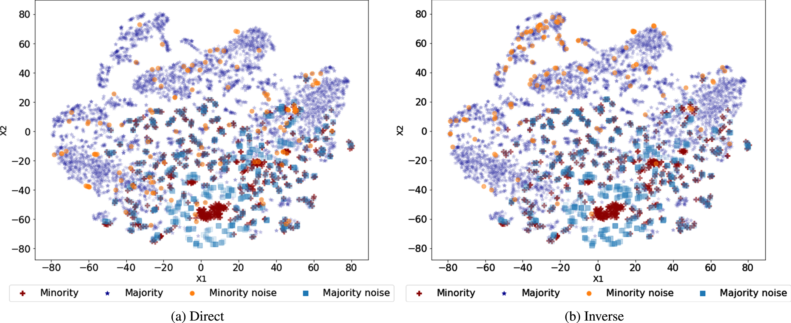
Distribution of noise injected dataset

For each dataset, noise-injected data were generated by varying the sampling probability to determine the sampling weight and noise level. In this study, the noise level was set from 10 % to 40 % with 10 % intervals.

4.3 Results

4.3.1 Noise-filtering results

The excessive elimination of samples in the minority class is one of the main problems arising when using AdaBoost algorithms combined with noise-filtering for imbalanced data. Therefore, before comparing the classification performances of the different noise-filtering methods, we checked the proportion of the samples defined as containing noise for each method. Tables 2 and 3 correspondingly show the differences in the percentages of noisy samples between the noise-filtering methods compared here and the proposed noise-filtering method with different cases for the original data based on ORBoost and RUSBoostWO. Here, negative values denote an increase in the number of noisy samples when using the proposed method.

Table 2
Difference in the percentage of the noisy samples between the proposed and comparison noise-filtering methods: ORBoost

Dataset Case 1 Case 2

Minority Majority All Minority Majority All

KC1 83.67% 4.57% 25.13% 83.66% 4.00% 24.70%

Ecoli 52.70% -12.17% -5.41% 31.42% -11.77% -7.27%

Satimage 50.51% 7.81% 11.97% 50.33% 8.30% 12.38%

Abalone 2.17% -0.28% -0.05% 1.31% -0.01% 0.12%

Spectrometer 33.50% -8.34% -4.80% 30.95% -10.48% -6.96%

US Crime 79.22% -9.48% -2.81% 60.13% -13.09% -7.58%

Credit Card 88.91% 1.79% 6.99% 88.95% 2.01% 7.19%

Oil 98.19% -8.16% -3.50% 97.99% -9.09% -4.40%

Wine Quality 93.22% -3.82% 0.42% 93.73% -4.96% -0.65%

Mammography 93.51% -0.27% 2.77% 93.58% -0.02% 3.00%

PC1 100.00% -0.05% 2.24% 100.00% -0.04% 2.25%

Dataset	Case 1	Case 2
KC1	83.67%	4.57%	25.13%	83.66%	4.00%	24.70%
Ecoli	52.70%	-12.17%	-5.41%	31.42%	-11.77%	-7.27%
Satimage	50.51%	7.81%	11.97%	50.33%	8.30%	12.38%
Abalone	2.17%	-0.28%	-0.05%	1.31%	-0.01%	0.12%
Spectrometer	33.50%	-8.34%	-4.80%	30.95%	-10.48%	-6.96%
US Crime	79.22%	-9.48%	-2.81%	60.13%	-13.09%	-7.58%
Credit Card	88.91%	1.79%	6.99%	88.95%	2.01%	7.19%
Oil	98.19%	-8.16%	-3.50%	97.99%	-9.09%	-4.40%
Wine Quality	93.22%	-3.82%	0.42%	93.73%	-4.96%	-0.65%
Mammography	93.51%	-0.27%	2.77%	93.58%	-0.02%	3.00%
PC1	100.00%	-0.05%	2.24%	100.00%	-0.04%	2.25%

Table 3

Difference in the percentage of the noisy samples between the proposed and comparison noise-filtering methods: RUSBoostWO

Dataset	Case 1			Case 2
	Minority	Majority	All	Minority	Majority	All
KC1	53.96%	3.44%	16.57%	59.21%	9.34%	22.30%
Ecoli	15.39%	-9.49%	-6.90%	19.77%	-7.37%	-4.55%
Satimage	4.47%	-1.70%	-1.10%	4.24%	-0.44%	0.01%
Abalone	0.06%	-0.90%	-0.81%	0.38%	0.02%	0.05%
Spectrometer	19.82%	-3.06%	-1.12%	17.36%	-12.22%	-9.71%
US Crime	16.25%	-7.20%	-5.44%	21.14%	-3.21%	-1.38%
Credit Card	17.24%	0.63%	1.62%	17.35%	0.96%	1.93%
Oil	31.67%	-3.06%	-1.54%	30.99%	-0.76%	0.63%
Wine Quality	19.38%	-1.29%	-0.39%	19.31%	-6.18%	-5.06%
Mammography	45.34%	6.40%	7.66%	45.65%	6.98%	8.24%
PC1	0.29%	-2.65%	-2.59%	0.31%	0.05%	0.06%

In Table 2, the difference in the percentage of the noisy minority samples between the proposed and comparison noise-filtering methods is considerably larger than the difference in the percentage of the noisy majority samples, and the percentage of the noisy samples in the minority class by the proposed method is smaller than that by the comparison method. For some datasets such as Oil, Wine Quality, Mammography, and PC1, the difference in the percentage of minority noisy samples was more than 90 %. This is because most of the samples defined as noise by Base are in the minority class, in contrast to the proposed method. In particular, in the datasets in which the weights of most minority samples are larger than those of the majority samples, the probability that the minority sample is discriminated as noise increases, and the difference in the proportion of the noisy minority samples between the proposed and comparison methods increases. For some datasets, the proportion of the noisy samples by the proposed method increased compared to that by the comparison method, but not by much. The difference between Case 1 and Case 2 is not significant.

Comparing Table 3 with Table 2, the difference in the percentage of the noisy samples between the proposed and comparison methods decreases when using RUSBoostWO compared to ORBoost. The difference in the percentage of minority noisy samples did not exceeds 50 %. For PC1, the difference decreases from 100 % to 0.30 %. This may be because RUSBoostWO detects noisy samples after the size of the majority class is reduced through under-sampling. In conclusion, when considering the characteristics of imbalanced data, where typically the degree of classification complexity for each class differs, the number of minority noisy samples decreases. In other words, the proposed noise-filtering method effectively prevents the excessive elimination of minority samples. It can also be expected to decrease the computation time if the number of majority noisy samples increases. Moreover, the similar conclusion can be drawn from the results for the noise-injected datasets, which are presented in Section S2.1 of the supplementary material.

4.3.2 Classification performance for the original datasets

Table 4 shows the average AUROC values when using the different base models (ORBoost and RUSBoostWO) for each dataset. Here, the “Base” and “AdaBoost” columns show the results using ORBoost or RUSBoostWO and AdaBoost, respectively. The best case for each base model is shown in bold. The standard deviation was calculated from the average AUROC values for each five-fold cross-validation. We also validated the performance of the proposed method using pairwise t-tests. The information about significantly better or worse performance compared to the AdaBoost and Base models at a significance level of 0.05 is represented by ↑ (better) and ↓ (worse) as superscripts for each average AUROC value of the proposed method. If the results of the t-tests are insignificant, •is used as the superscript. Among the two superscripts, the first represents the result of thet-test with AdaBoost and the second represents the result of the t-test with Base. The detailed results of the pairwise t-tests for the original datasets are provided in Section S1 of the supplementary material which also includes the results of the pairwise t-tests in terms of other classification metrics such as precision, recall, F1, and G-mean.

Table 4
Evaluation results for the original datasets in terms of AUROC

Dataset With noise-filtering

AdaBoost ORBoost RUSBoostWO

Base Case 1 Case 2 Base Case 1 Case 2

KC1 0.6481 0.6610 0.6481^•↓ 0.6479^•↓ 0.6667 0 . 6631^↑• 0 . 6465^•↓

(0.0109) (0.0096) (0.0108) (0.0106) (0.0096) (0.0120) (0.0143)

Ecoli 0.8928 0.9149 0.9260 ^↑↑ 0 . 9253^↑↑ 0.9271 0.9281 ^↑• 0 . 9262^↑•

(0.0194) (0.0145) (0.0147) (0.0107) (0.0131) (0.0129) (0.0114)

Satimage 0.9329 0.8884 0.9343 ^↑↑ 0 . 9335^•↑ 0.9306 0.9332 ^•↑ 0.9314^↓•

(0.0024) (0.0077) (0.0025) (0.0020) (0.0030) (0.0025) (0.0022)

Abalone 0.8497 0.8482 0.8512 ^↑↑ 0.8506^•↑ 0.8467 0 . 8460^↓• 0.8443^↓↓

(0.0036) (0.0034) (0.0034)) (0.0040)) (0.0041) (0.0037)) (0.0041))

Spectrometer 0.9615 0.9282 0.9570 ^•↑ 0.9412^↑↓ 0.9560 0.9591 ^•• 0.9345^↓↓

(0.0147) (0.0212) (0.0083) (0.0105) (0.0120) (0.0092) (0.0134)

US Crime 0.8779 0.8944 0.9105 ^↑↑ 0 . 9083^↑↑ 0.9092 0.9130 ^↑↑ 0.9100^↑•

(0.013) (0.0094) (0.0053) (0.0057) (0.0046) (0.0046) (0.0065)

Credit Card 0.9374 0.8648 0.9375^↑↑ 0.9376 ^↑↑ 0.9232 0.9377 ^↑↑ 0.9377 ^↑↑

(0.0002) (0.0053) (0.0002) (0.0002) (0.0023) (0.0002) (0.0002)

Oil 0.8288 0.7220 0.8946 ^↑↑ 0.8888^↑↑ 0.8883 0.8991 ^↑↑ 0.8942^↑•

(0.0417) (0.0120) (0.0197) (0.0231) (0.0150) (0.0197) (0.0239)

Wine Quality 0.8026 0.7420 0.8206 ^↑↑ 0.8171^↑↑ 0.8198 0.8131^↑↓ 0.8152^↑•

(0.0102) (0.0178) (0.0092) (0.0121) (0.0103) (0.0130) (0.0121)

Mammography 0.9345 0.6919 0.9362 ^↑↑ 0 . 9361^↑↑ 0.9100 0 . 9326^•↑ 0.9335 ^•↑

(0.0043) (0.0047) (0.0043) (0.0044) (0.0032) (0.0046) (0.0038)

PC1 0.7375 0.6199 0.7375 ^•↑ 0.7375^•↑ 0.7289 0.7376 ^•↑ 0.7322^↓•

(0.0110) (0.0151) (0.0125) (0.0107) (0.0123) (0.0097) (0.0160)

Dataset		With noise-filtering
KC1	0.6481	0.6610	0.6481^•↓	0.6479^•↓	0.6667	0 . 6631^↑•	0 . 6465^•↓
	(0.0109)	(0.0096)	(0.0108)	(0.0106)	(0.0096)	(0.0120)	(0.0143)
Ecoli	0.8928	0.9149	0.9260 ^↑↑	0 . 9253^↑↑	0.9271	0.9281 ^↑•	0 . 9262^↑•
	(0.0194)	(0.0145)	(0.0147)	(0.0107)	(0.0131)	(0.0129)	(0.0114)
Satimage	0.9329	0.8884	0.9343 ^↑↑	0 . 9335^•↑	0.9306	0.9332 ^•↑	0.9314^↓•
	(0.0024)	(0.0077)	(0.0025)	(0.0020)	(0.0030)	(0.0025)	(0.0022)
Abalone	0.8497	0.8482	0.8512 ^↑↑	0.8506^•↑	0.8467	0 . 8460^↓•	0.8443^↓↓
	(0.0036)	(0.0034)	(0.0034))	(0.0040))	(0.0041)	(0.0037))	(0.0041))
Spectrometer	0.9615	0.9282	0.9570 ^•↑	0.9412^↑↓	0.9560	0.9591 ^••	0.9345^↓↓
	(0.0147)	(0.0212)	(0.0083)	(0.0105)	(0.0120)	(0.0092)	(0.0134)
US Crime	0.8779	0.8944	0.9105 ^↑↑	0 . 9083^↑↑	0.9092	0.9130 ^↑↑	0.9100^↑•
	(0.013)	(0.0094)	(0.0053)	(0.0057)	(0.0046)	(0.0046)	(0.0065)
Credit Card	0.9374	0.8648	0.9375^↑↑	0.9376 ^↑↑	0.9232	0.9377 ^↑↑	0.9377 ^↑↑
	(0.0002)	(0.0053)	(0.0002)	(0.0002)	(0.0023)	(0.0002)	(0.0002)
Oil	0.8288	0.7220	0.8946 ^↑↑	0.8888^↑↑	0.8883	0.8991 ^↑↑	0.8942^↑•
	(0.0417)	(0.0120)	(0.0197)	(0.0231)	(0.0150)	(0.0197)	(0.0239)
Wine Quality	0.8026	0.7420	0.8206 ^↑↑	0.8171^↑↑	0.8198	0.8131^↑↓	0.8152^↑•
	(0.0102)	(0.0178)	(0.0092)	(0.0121)	(0.0103)	(0.0130)	(0.0121)
Mammography	0.9345	0.6919	0.9362 ^↑↑	0 . 9361^↑↑	0.9100	0 . 9326^•↑	0.9335 ^•↑
	(0.0043)	(0.0047)	(0.0043)	(0.0044)	(0.0032)	(0.0046)	(0.0038)
PC1	0.7375	0.6199	0.7375 ^•↑	0.7375^•↑	0.7289	0.7376 ^•↑	0.7322^↓•
	(0.0110)	(0.0151)	(0.0125)	(0.0107)	(0.0123)	(0.0097)	(0.0160)

In Table 4, it is shown that the AdaBoost algorithms with noise-filtering always perform better than AdaBoost. In approximately half of the datasets, ORBoost and RUSBoostWO showed lower AUROC values than AdaBoost. ORBoost and RUSBoostWO perform the noise-filtering process regardless of whether noise exists in the dataset. Because the datasets used in this study were selected from among the well-known imbalanced datasets, the classification performance may be lowered by removing the samples defined as noise, if noise is not included in the datasets. However, when the propose noise-filtering method was used, the classification performance became better than that of Adaboost, even for the datasets where the performance of ORBoost or RUBBoostWO was lower than that of Adaboost.

The proposed method generally provides improved classification performance for ORBoost. It is demonstrated that the improved classification performance was observed for several datasets such as Ecoli, Satimage, Abalone, US Crime, Credit Card, Oil, Wine Quality, Mammography, and PC1. These datasets commonly have high IR values such that minority samples are likely to be defined as noise. Therefore, the effect of the prevention of the excessive elimination of minority samples as noise is considerable in these datasets, which improves the classification performance. However, less of an improvement was observed for the results of RUSBoostWO. The number of significantly improved cases decrease; in particular, this value decreases from 8 to 1 of Case 2. The classification performance of Base increases because the degree of IR is lessened via under-sampling before the noise-filtering method is applied.

The proposed method could not improve the classification performance of KC1. In this case, the IR value is smaller than those in the other datasets and the proposed noise-filtering method decreased the number of noisy samples for both minority and majority classes. When comparing the base models, the result of RUSBoostWO for KC1 was better than the result of ORBoost. Therefore it can be inferred that when the degree of IR is low, a decreased number of minority noisy samples cannot lead to an improvement in the classification performance.

4.3.3 Classification performance for the noise-injected datasets

Tables 5 and 7 show the evaluation results for the noise-injected datasets with different noise levels in terms of AUROC according to ORBoost and RUSBoost, based on the type of sampling probability, respectively. In these tables, the “Base” and “AdaBoost” columns show the results using ORBoost or RUSBoostWO and AdaBoost, respectively. The best cases for each noise level and type of base model are shown in bold. The information about significantly better or worse performance compared to the AdaBoost and Base models at a significance level of 0.05 is represented in the same way used for Table 4.

Table 5
Evaluation results for the noise-injected datasets in terms of AUROC: using p (x_i) ^direct

Dataset Noise Level AdaBoost ORBoost RUSBoostWO

Base Case 1 Case 2 Base Case 1 Case 2

KC1 10% 0.6516 0.6620 0.6517^•↓ 0.6517^•↓ 0.6706 0.6564^•↓ 0.6490^•↓

(0.0091) (0.0070) (0.0089) (0.0136) (0.0077) (0.0120) (0.0143)

20% 0.6525 0.6633 0.6532^•↓ 0.6532^•↓ 0.6709 0.6513^•↓ 0.6477^•↓

(0.0119) (0.0101) (0.0143) (0.0121) (0.0079) (0.0130) (0.0165)

30% 0.6452 0.6550 0.6476^•↓ 0.6500^↑• 0.6645 0.6446^•↓ 0.6441^•↓

(0.0109) (0.0100) (0.0118) (0.0108) (0.0084) (0.0095) (0.0158)

40% 0.6459 0.6589 0.6460^•↓ 0.6484^•↓ 0.6606 0.6447^•↓ 0.6501^•↓

(0.0122) (0.0144) (0.0120) (0.0100) (0.0105) (0.0145) (0.0136)

Ecoli 10% 0.8517 0.8852 0.9225 ^↑↑ 0.9141^↑↑ 0.9206 0.9262 ^↑• 0.9143^↑•

(0.0266) (0.0213) (0.0122) (0.0159) (0.0131) (0.0111) (0.0130)

20% 0.8693 0.8792 0.9151 ^↑↑ 0.9064^↑↑ 0.9185 0.9177^↑• 0.9123^↑•

(0.0251) (0.0231) (0.0133) (0.0179) (0.0181) (0.0155) (0.0168)

30% 0.8491 0.8647 0.9000 ^↑↑ 0.8831^↑↑ 0.8699 0.9070 ^↑↑ 0.9064^↑↑

(0.0271) (0.0223) (0.0218) (0.0245) (0.0377) (0.0156) (0.0173)

40% 0.8291 0.8448 0.9041 ^↑↑ 0.8617^↑• 0.8448 0.9082 ^↑↑ 0.8860^↑↑

(0.0364) (0.0419) (0.0201) (0.0402) (0.0355) (0.0156) (0.0259)

Satimage 10% 0.9227 0.9250 0.9252 ^•• 0.9189^↓↓ 0.9265 0.9239^•↓ 0.9178^↓↓

(0.0033) (0.0033) (0.0032) (0.0054) (0.0028) (0.0044) (0.0064)

20% 0.9177 0.9236 0.9177^•↓ 0.9193^•↓ 0.9210 0.9144^↓↓ 0.9162^•↓

(0.0030) (0.0037) (0.0026) (0.0040) (0.0036) (0.0040) (0.0036)

30% 0.9084 0.9133 0.9084^•↓ 0.9111^↑• 0.9116 0.9035^↓↓ 0.9076^•↓

(0.0050) (0.0074) (0.0050) (0.0042) (0.0039) (0.0049) (0.0054)

40% 0.9001 0.9065 0.9004^•↓ 0.9032^↑↓ 0.8976 0.8942^↓↓ 0.8988 ^••

(0.0037) (0.0044) (0.0034) (0.0040) (0.0043) (0.0049) (0.0075)

Abalone 10% 0.8481 0.8486 0.8481^•• 0.8479^•• 0.8420 0.8429 ^↓• 0.8419^↓•

(0.0043) (0.0039) (0.0043) (0.0036) (0.0045) (0.0051) (0.0041)

20% 0.8433 0.8448 0.8434^•• 0.8443^•• 0.8398 0.8412 ^•• 0.8394^↓•

(0.0038) (0.0037) (0.0038) (0.0034) (0.0046) (0.0040) (0.0061)

30% 0.8394 0.8414 0.8396^•↓ 0.8396^•• 0.8349 0.8344^↓• 0.8372 ^••

(0.0050) (0.0048) (0.0052) (0.0063) (0.0045) (0.0058) (0.0051)

40% 0.8361 0.8376 0.8362^•• 0.8368^•• 0.8288 0.8279^↓• 0.8324 ^↓↑

(0.0070) (0.0048) (0.0071) (0.0053) (0.0071) (0.0068) (0.0062)

Spectrometer 10% 0.9212 0.9135 0.9451 ^•↓ 0.9343^•↓ 0.9572 0.9496^•↓ 0.9139^•↓

(0.0225) (0.0331) (0.0146) (0.0188) (0.0101) (0.0103) (0.0325)

20% 0.8898 0.9044 0.9169 ^•↓ 0.9043^•↓ 0.9353 0.9366 ^•↓ 0.9180^•↓

(0.0269) (0.0259) (0.0251) (0.0276) (0.0237) (0.0204) (0.0222)

30% 0.8664 0.8863 0.9025 ^•↓ 0.8860^↑• 0.8929 0.9041 ^•↓ 0.8979^•↓

(0.0284) (0.0273) (0.0377) (0.0303) (0.0303) (0.0267) (0.0325)

40% 0.8273 0.8753 0.8512^•↓ 0.8624^•↓ 0.8663 0.8851 ^•↓ 0.8669^•↓

(0.0414) (0.0340) (0.0314) (0.0355) (0.0408) (0.0311) (0.0354)

US Crime 10% 0.8603 0.8988 0.9082 ^↑↑ 0.9018^↑↑ 0.9018 0.9110 ^↑• 0.9068^↑•

(0.0102) (0.0082) (0.0053) (0.0078) (0.0062) (0.0049) (0.0064)

20% 0.8471 0.8941 0.8926^↑↑ 0.8782^↑↑ 0.8907 0.8933^↑• 0.9012 ^↑•

(0.0138) (0.0076) (0.0087) (0.0158) (0.0146) (0.0068) (0.0081)

30% 0.8334 0.8785 0.8976 ^↑↑ 0.8525^↑↑ 0.8786 0.9002 ^↑↑ 0.8644^↑↑

(0.0134) (0.0211) (0.0093) (0.0150) (0.0122) (0.0075) (0.0181)

40% 0.8162 0.8606 0.8560^↑↑ 0.8386^↑• 0.8659 0.8910 ^↑↑ 0.8334^↑↑

(0.0156) (0.0270) (0.0206) (0.0166) (0.0209) (0.0098) (0.0180)

Credit Card 10% 0.9364 0.8806 0.9368 ^•• 0.9366^↓↓ 0.9357 0.9371 ^•↓ 0.9370^↓↓

(0.0004) (0.0009) (0.0003) (0.0004) (0.0002) (0.0002) (0.0003)

20% 0.9356 0.8806 0.9361 ^•↓ 0.9361 ^•↓ 0.9355 0.9363 ^↓↓ 0.9362^•↓

(0.0003) (0.0029) (0.0003) (0.0003) (0.0004) (0.0003) (0.0003)

30% 0.9346 0.8853 0.9349 ^•↓ 0.9349 ^↑• 0.9345 0.9349 ^↓↓ 0.9347^•↓

(0.0003) (0.0061) (0.0003) (0.0004) (0.0004) (0.0003) (0.0004)

40% 0.9331 0.8806 0.9331^•↓ 0.9333 ^↑↓ 0.9333 0.9334 ^↓↓ 0.9334 ^••

(0.0003) (0.0033) (0.0003) (0.0003) (0.0004) (0.0004) (0.0006)

Oil 10% 0.8355 0.7835 0.8775 ^•• 0.8758^•• 0.8791 0.8881 ^↓• 0.8803^↓•

(0.0457) (0.0272) (0.0275) (0.0257) (0.0237) (0.0182) (0.0280)

20% 0.8196 0.8327 0.8733 ^•• 0.8554^•• 0.8647 0.8804 ^•• 0.8695^↓•

(0.0383) (0.0284) (0.0231) (0.0350) (0.0220) (0.0266) (0.0302)

30% 0.7685 0.8107 0.8395 ^•↓ 0.8128^•• 0.8153 0.8685 ^↓• 0.8532^••

(0.0419) (0.0334) (0.0336) (0.0379) (0.0415) (0.0232) (0.0421)

40% 0.7827 0.8080 0.8385 ^•• 0.8116^•• 0.8233 0.8543 ^↓• 0.8340^↓↑

(0.0370) (0.0269) (0.0315) (0.0456) (0.0420) (0.0261) (0.0325)

Wine Quality 10% 0.7835 0.7517 0.8016^•↓ 0.8030 ^•↓ 0.8074 0.8084 ^•↓ 0.8035^•↓

(0.0151) (0.0192) (0.0128) (0.0128) (0.0120) (0.0125) (0.0118)

20% 0.7775 0.7445 0.7837^•↓ 0.7914 ^•↓ 0.7963 0.7876^•↓ 0.7966 ^•↓

(0.0133) (0.0187) (0.0153) (0.0118) (0.0126) (0.0122) (0.0133)

30% 0.7597 0.7432 0.7822 ^•↓ 0.7738^↑• 0.7651 0.7802^•↓ 0.7827 ^•↓

(0.0152) (0.0208) (0.0201) (0.0166) (0.0142) (0.0135) (0.0164)

40% 0.7571 0.7384 0.7709 ^•↓ 0.7701^•↓ 0.7530 0.7840 ^•↓ 0.7738^•↓

(0.0155) (0.0226) (0.0140) (0.0182) (0.0159) (0.0187) (0.0147)

Mammography 10% 0.9272 0.6880 0.9286^↑↑ 0.9294 ^↑↑ 0.9136 0.9248^↑• 0.9251 ^↑•

(0.0047) (0.0080) (0.0047) (0.0052) (0.0039) (0.0060) (0.0051)

20% 0.9236 0.6883 0.9250 ^↑↑ 0.9250 ^↑↑ 0.9192 0.9212 ^↑• 0.9202^↑•

(0.0060) (0.0061) (0.0064) (0.0068) (0.0076) (0.0067) (0.0057)

30% 0.9160 0.6892 0.9173 ^↑↑ 0.9173 ^↑↑ 0.9127 0.9137 ^↑↑ 0.9122^↑↑

(0.0059) (0.0083) (0.0067) (0.0065) (0.0041) (0.0081) (0.0073)

40% 0.9070 0.6982 0.9087^↑↑ 0.9095 ^↑• 0.9044 0.9036^↑↑ 0.9036^↑↑

(0.0068) (0.0146) (0.0070) (0.0072) (0.0069) (0.0084) (0.0100)

PC1 10% 0.7391 0.6101 0.7394^•• 0.7397 ^↓↓ 0.7267 0.7290^•↓ 0.7346 ^↓↓

(0.0121) (0.0212) (0.0121) (0.0128) (0.0146) (0.0110) (0.0168)

20% 0.7303 0.5878 0.7323 ^•↓ 0.7312^•↓ 0.7140 0.7208^↓↓ 0.7249 ^•↓

(0.0106) (0.0178) (0.0127) (0.0119) (0.0161) (0.0163) (0.0161)

30% 0.7248 0.5714 0.7251^•↓ 0.7266 ^↑• 0.7058 0.7171 ^↓↓ 0.7097^•↓

(0.0143) (0.0160) (0.0145) (0.0151) (0.0166) (0.0196) (0.0200)

40% 0.7152 0.5634 0.7157 ^•↓ 0.7151^↑↓ 0.6967 0.6960^↓↓ 0.6987 ^••

(0.0145) (0.0118) (0.0149) (0.0128) (0.0177) (0.0197) (0.0216)

Dataset	Noise Level	AdaBoost	ORBoost	RUSBoostWO
KC1	10%	0.6516	0.6620	0.6517^•↓	0.6517^•↓	0.6706	0.6564^•↓	0.6490^•↓
		(0.0091)	(0.0070)	(0.0089)	(0.0136)	(0.0077)	(0.0120)	(0.0143)
	20%	0.6525	0.6633	0.6532^•↓	0.6532^•↓	0.6709	0.6513^•↓	0.6477^•↓
		(0.0119)	(0.0101)	(0.0143)	(0.0121)	(0.0079)	(0.0130)	(0.0165)
	30%	0.6452	0.6550	0.6476^•↓	0.6500^↑•	0.6645	0.6446^•↓	0.6441^•↓
		(0.0109)	(0.0100)	(0.0118)	(0.0108)	(0.0084)	(0.0095)	(0.0158)
	40%	0.6459	0.6589	0.6460^•↓	0.6484^•↓	0.6606	0.6447^•↓	0.6501^•↓
		(0.0122)	(0.0144)	(0.0120)	(0.0100)	(0.0105)	(0.0145)	(0.0136)
Ecoli	10%	0.8517	0.8852	0.9225 ^↑↑	0.9141^↑↑	0.9206	0.9262 ^↑•	0.9143^↑•
		(0.0266)	(0.0213)	(0.0122)	(0.0159)	(0.0131)	(0.0111)	(0.0130)
	20%	0.8693	0.8792	0.9151 ^↑↑	0.9064^↑↑	0.9185	0.9177^↑•	0.9123^↑•
		(0.0251)	(0.0231)	(0.0133)	(0.0179)	(0.0181)	(0.0155)	(0.0168)
	30%	0.8491	0.8647	0.9000 ^↑↑	0.8831^↑↑	0.8699	0.9070 ^↑↑	0.9064^↑↑
		(0.0271)	(0.0223)	(0.0218)	(0.0245)	(0.0377)	(0.0156)	(0.0173)
	40%	0.8291	0.8448	0.9041 ^↑↑	0.8617^↑•	0.8448	0.9082 ^↑↑	0.8860^↑↑
		(0.0364)	(0.0419)	(0.0201)	(0.0402)	(0.0355)	(0.0156)	(0.0259)
Satimage	10%	0.9227	0.9250	0.9252 ^••	0.9189^↓↓	0.9265	0.9239^•↓	0.9178^↓↓
		(0.0033)	(0.0033)	(0.0032)	(0.0054)	(0.0028)	(0.0044)	(0.0064)
	20%	0.9177	0.9236	0.9177^•↓	0.9193^•↓	0.9210	0.9144^↓↓	0.9162^•↓
		(0.0030)	(0.0037)	(0.0026)	(0.0040)	(0.0036)	(0.0040)	(0.0036)
	30%	0.9084	0.9133	0.9084^•↓	0.9111^↑•	0.9116	0.9035^↓↓	0.9076^•↓
		(0.0050)	(0.0074)	(0.0050)	(0.0042)	(0.0039)	(0.0049)	(0.0054)
	40%	0.9001	0.9065	0.9004^•↓	0.9032^↑↓	0.8976	0.8942^↓↓	0.8988 ^••
		(0.0037)	(0.0044)	(0.0034)	(0.0040)	(0.0043)	(0.0049)	(0.0075)
Abalone	10%	0.8481	0.8486	0.8481^••	0.8479^••	0.8420	0.8429 ^↓•	0.8419^↓•
		(0.0043)	(0.0039)	(0.0043)	(0.0036)	(0.0045)	(0.0051)	(0.0041)
	20%	0.8433	0.8448	0.8434^••	0.8443^••	0.8398	0.8412 ^••	0.8394^↓•
		(0.0038)	(0.0037)	(0.0038)	(0.0034)	(0.0046)	(0.0040)	(0.0061)
	30%	0.8394	0.8414	0.8396^•↓	0.8396^••	0.8349	0.8344^↓•	0.8372 ^••
		(0.0050)	(0.0048)	(0.0052)	(0.0063)	(0.0045)	(0.0058)	(0.0051)
	40%	0.8361	0.8376	0.8362^••	0.8368^••	0.8288	0.8279^↓•	0.8324 ^↓↑
		(0.0070)	(0.0048)	(0.0071)	(0.0053)	(0.0071)	(0.0068)	(0.0062)
Spectrometer	10%	0.9212	0.9135	0.9451 ^•↓	0.9343^•↓	0.9572	0.9496^•↓	0.9139^•↓
		(0.0225)	(0.0331)	(0.0146)	(0.0188)	(0.0101)	(0.0103)	(0.0325)
	20%	0.8898	0.9044	0.9169 ^•↓	0.9043^•↓	0.9353	0.9366 ^•↓	0.9180^•↓
		(0.0269)	(0.0259)	(0.0251)	(0.0276)	(0.0237)	(0.0204)	(0.0222)
	30%	0.8664	0.8863	0.9025 ^•↓	0.8860^↑•	0.8929	0.9041 ^•↓	0.8979^•↓
		(0.0284)	(0.0273)	(0.0377)	(0.0303)	(0.0303)	(0.0267)	(0.0325)
	40%	0.8273	0.8753	0.8512^•↓	0.8624^•↓	0.8663	0.8851 ^•↓	0.8669^•↓
		(0.0414)	(0.0340)	(0.0314)	(0.0355)	(0.0408)	(0.0311)	(0.0354)
US Crime	10%	0.8603	0.8988	0.9082 ^↑↑	0.9018^↑↑	0.9018	0.9110 ^↑•	0.9068^↑•
		(0.0102)	(0.0082)	(0.0053)	(0.0078)	(0.0062)	(0.0049)	(0.0064)
	20%	0.8471	0.8941	0.8926^↑↑	0.8782^↑↑	0.8907	0.8933^↑•	0.9012 ^↑•
		(0.0138)	(0.0076)	(0.0087)	(0.0158)	(0.0146)	(0.0068)	(0.0081)
	30%	0.8334	0.8785	0.8976 ^↑↑	0.8525^↑↑	0.8786	0.9002 ^↑↑	0.8644^↑↑
		(0.0134)	(0.0211)	(0.0093)	(0.0150)	(0.0122)	(0.0075)	(0.0181)
	40%	0.8162	0.8606	0.8560^↑↑	0.8386^↑•	0.8659	0.8910 ^↑↑	0.8334^↑↑
		(0.0156)	(0.0270)	(0.0206)	(0.0166)	(0.0209)	(0.0098)	(0.0180)
Credit Card	10%	0.9364	0.8806	0.9368 ^••	0.9366^↓↓	0.9357	0.9371 ^•↓	0.9370^↓↓
		(0.0004)	(0.0009)	(0.0003)	(0.0004)	(0.0002)	(0.0002)	(0.0003)
	20%	0.9356	0.8806	0.9361 ^•↓	0.9361 ^•↓	0.9355	0.9363 ^↓↓	0.9362^•↓
		(0.0003)	(0.0029)	(0.0003)	(0.0003)	(0.0004)	(0.0003)	(0.0003)
	30%	0.9346	0.8853	0.9349 ^•↓	0.9349 ^↑•	0.9345	0.9349 ^↓↓	0.9347^•↓
		(0.0003)	(0.0061)	(0.0003)	(0.0004)	(0.0004)	(0.0003)	(0.0004)
	40%	0.9331	0.8806	0.9331^•↓	0.9333 ^↑↓	0.9333	0.9334 ^↓↓	0.9334 ^••
		(0.0003)	(0.0033)	(0.0003)	(0.0003)	(0.0004)	(0.0004)	(0.0006)
Oil	10%	0.8355	0.7835	0.8775 ^••	0.8758^••	0.8791	0.8881 ^↓•	0.8803^↓•
		(0.0457)	(0.0272)	(0.0275)	(0.0257)	(0.0237)	(0.0182)	(0.0280)
	20%	0.8196	0.8327	0.8733 ^••	0.8554^••	0.8647	0.8804 ^••	0.8695^↓•
		(0.0383)	(0.0284)	(0.0231)	(0.0350)	(0.0220)	(0.0266)	(0.0302)
	30%	0.7685	0.8107	0.8395 ^•↓	0.8128^••	0.8153	0.8685 ^↓•	0.8532^••
		(0.0419)	(0.0334)	(0.0336)	(0.0379)	(0.0415)	(0.0232)	(0.0421)
	40%	0.7827	0.8080	0.8385 ^••	0.8116^••	0.8233	0.8543 ^↓•	0.8340^↓↑
		(0.0370)	(0.0269)	(0.0315)	(0.0456)	(0.0420)	(0.0261)	(0.0325)
Wine Quality	10%	0.7835	0.7517	0.8016^•↓	0.8030 ^•↓	0.8074	0.8084 ^•↓	0.8035^•↓
		(0.0151)	(0.0192)	(0.0128)	(0.0128)	(0.0120)	(0.0125)	(0.0118)
	20%	0.7775	0.7445	0.7837^•↓	0.7914 ^•↓	0.7963	0.7876^•↓	0.7966 ^•↓
		(0.0133)	(0.0187)	(0.0153)	(0.0118)	(0.0126)	(0.0122)	(0.0133)
	30%	0.7597	0.7432	0.7822 ^•↓	0.7738^↑•	0.7651	0.7802^•↓	0.7827 ^•↓
		(0.0152)	(0.0208)	(0.0201)	(0.0166)	(0.0142)	(0.0135)	(0.0164)
	40%	0.7571	0.7384	0.7709 ^•↓	0.7701^•↓	0.7530	0.7840 ^•↓	0.7738^•↓
		(0.0155)	(0.0226)	(0.0140)	(0.0182)	(0.0159)	(0.0187)	(0.0147)
Mammography	10%	0.9272	0.6880	0.9286^↑↑	0.9294 ^↑↑	0.9136	0.9248^↑•	0.9251 ^↑•
		(0.0047)	(0.0080)	(0.0047)	(0.0052)	(0.0039)	(0.0060)	(0.0051)
	20%	0.9236	0.6883	0.9250 ^↑↑	0.9250 ^↑↑	0.9192	0.9212 ^↑•	0.9202^↑•
		(0.0060)	(0.0061)	(0.0064)	(0.0068)	(0.0076)	(0.0067)	(0.0057)
	30%	0.9160	0.6892	0.9173 ^↑↑	0.9173 ^↑↑	0.9127	0.9137 ^↑↑	0.9122^↑↑
		(0.0059)	(0.0083)	(0.0067)	(0.0065)	(0.0041)	(0.0081)	(0.0073)
	40%	0.9070	0.6982	0.9087^↑↑	0.9095 ^↑•	0.9044	0.9036^↑↑	0.9036^↑↑
		(0.0068)	(0.0146)	(0.0070)	(0.0072)	(0.0069)	(0.0084)	(0.0100)
PC1	10%	0.7391	0.6101	0.7394^••	0.7397 ^↓↓	0.7267	0.7290^•↓	0.7346 ^↓↓
		(0.0121)	(0.0212)	(0.0121)	(0.0128)	(0.0146)	(0.0110)	(0.0168)
	20%	0.7303	0.5878	0.7323 ^•↓	0.7312^•↓	0.7140	0.7208^↓↓	0.7249 ^•↓
		(0.0106)	(0.0178)	(0.0127)	(0.0119)	(0.0161)	(0.0163)	(0.0161)
	30%	0.7248	0.5714	0.7251^•↓	0.7266 ^↑•	0.7058	0.7171 ^↓↓	0.7097^•↓
		(0.0143)	(0.0160)	(0.0145)	(0.0151)	(0.0166)	(0.0196)	(0.0200)
	40%	0.7152	0.5634	0.7157 ^•↓	0.7151^↑↓	0.6967	0.6960^↓↓	0.6987 ^••
		(0.0145)	(0.0118)	(0.0149)	(0.0128)	(0.0177)	(0.0197)	(0.0216)

Table 6

Evaluation results for the noise-injected datasets in terms of AUROC: using p (x_i) ^inverse

Dataset	Noise Level	AdaBoost	ORBoost			RUSBoostWO
			Base	Case 1	Case 2	Base	Case 1	Case 2
KC1	10%	0.6424	0.6665	0.6430^•↓	0.6439^•↓	0.6728	0.6425^•↓	0.6445^•↓
		(0.0111)	(0.0085)	(0.0114)	(0.0138)	(0.0081)	(0.0145)	(0.0137)
	20%	0.6274	0.6526	0.6289^•↓	0.6286^•↓	0.6527	0.6240^•↓	0.6283^•↓
		(0.0111)	(0.0130)	(0.0115)	(0.0095)	(0.0137)	(0.0140)	(0.0157)
	30%	0.6159	0.6452	0.6182^•↓	0.6187^•↓	0.6223	0.6107^•↓	0.6167^••
		(0.0156)	(0.0165)	(0.0151)	(0.0147)	(0.0152)	(0.0154)	(0.0185)
	40%	0.5997	0.6056	0.6007^••	0.6026^••	0.5896	0.5975 ^••	0.5994^•↑
		(0.0164)	(0.0247)	(0.0177)	(0.0124)	(0.0190)	(0.0189)	(0.0162)
Ecoli	10%	0.8396	0.8851	0.9166 ^↑↑	0.9068^↑↑	0.9172	0.9221 ^↑•	0.9119^↑•
		(0.0236)	(0.0220)	(0.0106)	(0.0200)	(0.0153)	(0.0093)	(0.0185)
	20%	0.8287	0.8516	0.8953 ^↑↑	0.8816^↑↑	0.8582	0.9050 ^↑↑	0.8930^↑↑
		(0.0208)	(0.0475)	(0.0228)	(0.0238)	(0.0366)	(0.0200)	(0.0253)
	30%	0.8316	0.8390	0.8987 ^↑↑	0.8608^↑↑	0.8327	0.9040 ^↑↑	0.8854^↑↑
		(0.0288)	(0.0256)	(0.0239)	(0.0261)	(0.0401)	(0.0196)	(0.0341)
	40%	0.7900	0.7928	0.8427 ^↑↑	0.8029^••	0.7731	0.8491 ^↑↑	0.8036^•↑
		(0.0317)	(0.0340)	(0.0422)	(0.0342)	(0.0354)	(0.0530)	(0.0474)
Satimage	10%	0.9149	0.9249	0.9149^•↓	0.9149^•↓	0.9237	0.9137^•↓	0.9131^•↓
		(0.0044)	(0.0032)	(0.0042)	(0.0043)	(0.0036)	(0.0036)	(0.0048)
	20%	0.9041	0.9066	0.9041^•↓	0.9049^••	0.9075	0.9004^↓↓	0.9055^••
		(0.0035)	(0.0047)	(0.0037)	(0.0047)	(0.0054)	(0.0053)	(0.0048)
	30%	0.8846	0.8933	0.8850^•↓	0.8889^↑↓	0.8828	0.8801^↓↓	0.8859^••
		(0.0041)	(0.0073)	(0.0047)	(0.0052)	(0.0041)	(0.0051)	(0.0061)
	40%	0.8662	0.8676	0.8663^••	0.8664^••	0.8643	0.8591^↓•	0.8610^↓•
		(0.0051)	(0.0055)	(0.0051)	(0.0047)	(0.0212)	(0.0065)	(0.0084)
Abalone	10%	0.8472	0.8473	0.8473 ^••	0.8476^••	0.8425	0.8414^↓•	0.8412^↓•
		(0.0035)	(0.0042)	(0.0033)	(0.0034)	(0.0040)	(0.0052)	(0.0058)
	20%	0.8398	0.8424	0.8399^•↓	0.8408^••	0.8370	0.8340^↓↓	0.8346^↓•
		(0.0040)	(0.0027)	(0.0040)	(0.0041)	(0.0048)	(0.0053)	(0.0057)
	30%	0.8313	0.8317	0.8314^••	0.8325^↑•	0.8222	0.8229 ^↓•	0.8245^↓•
		(0.0060)	(0.0058)	(0.0060)	(0.0050)	(0.0064)	(0.0052)	(0.0084)
	40%	0.8181	0.8183	0.8184 ^••	0.8184^••	0.8231	0.8078^↓↓	0.8156^•↓
		(0.0068)	(0.0065)	(0.0066)	(0.0073)	(0.0158)	(0.0072)	(0.0106)
Spectrometer	10%	0.9166	0.8888	0.9419 ^•↓	0.9260^•↓	0.9547	0.9528^•↓	0.9135^•↓
		(0.0264)	(0.0376)	(0.0224)	(0.0239)	(0.0132)	(0.0108)	(0.0233)
	20%	0.8825	0.8906	0.9186 ^•↓	0.8995^•↓	0.9010	0.9232 ^•↓	0.8981^•↓
		(0.0292)	(0.0248)	(0.0252)	(0.0254)	(0.0214)	(0.0304)	(0.0345)
	30%	0.8480	0.8584	0.8662 ^•↓	0.8640^•↓	0.8512	0.8858 ^•↓	0.8658^••
		(0.0358)	(0.0404)	(0.0391)	(0.0327)	(0.0259)	(0.0289)	(0.0353)
	40%	0.8092	0.8292	0.8188^••	0.8289^••	0.8160	0.8299 ^••	0.8249^•↑
		(0.0381)	(0.0402)	(0.0389)	(0.0282)	(0.0340)	(0.0273)	(0.0485)
US Crime	10%	0.8522	0.8990	0.9077 ^↑↑	0.8994^↑↑	0.9050	0.9090 ^↑•	0.9014^↑•
		(0.0142)	(0.0063)	(0.0051)	(0.0077)	(0.0072)	(0.0054)	(0.0094)
	20%	0.8404	0.8903	0.8950 ^↑↑	0.8671^↑↑	0.8828	0.8952 ^↑↑	0.8953^↑↑
		(0.0158)	(0.0140)	(0.0077)	(0.0189)	(0.0115)	(0.0066)	(0.0115)
	30%	0.8245	0.8563	0.8906 ^↑↑	0.8358^↑↑	0.8610	0.8967 ^↑↑	0.8356^↑↑
		(0.0140)	(0.0311)	(0.0098)	(0.0123)	(0.0255)	(0.0079)	(0.0168)
	40%	0.7966	0.8215	0.8095^↑↑	0.8166^••	0.8338	0.8698 ^↑↑	0.8045^•↑
		(0.0147)	(0.0227)	(0.0195)	(0.0136)	(0.0326)	(0.0219)	(0.0172)
Credit Card	10%	0.9302	0.8783	0.9307 ^•↓	0.9308^•↓	0.9303	0.9313 ^•↓	0.9318^•↓
		(0.0004)	(0.0018)	(0.0004)	(0.0005)	(0.0005)	(0.0005)	(0.0005)
	20%	0.9204	0.8729	0.9204 ^•↓	0.9206^••	0.9203	0.9203 ^↓↓	0.9203^••
		(0.0008)	(0.0056)	(0.0008)	(0.0008)	(0.0009)	(0.0008)	(0.0007)
	30%	0.9042	0.8961	0.9042 ^•↓	0.9042^↑↓	0.9041	0.9038^↓↓	0.9040^••
		(0.0014)	(0.0050)	(0.0014)	(0.0013)	(0.0012)	(0.0012)	(0.0015)
	40%	0.8769	0.8772	0.8771^••	0.8769^••	0.8769	0.8767^↓•	0.8768^↓•
		(0.0018)	(0.0022)	(0.0019)	(0.0023)	(0.0023)	(0.0023)	(0.0022)
Oil	10%	0.8310	0.8098	0.8721 ^••	0.8655^••	0.8844	0.8947 ^↓•	0.8774^↓•
		(0.0350)	(0.0263)	(0.0349)	(0.0220)	(0.0254)	(0.0211)	(0.0218)
	20%	0.8053	0.8003	0.8516 ^•↓	0.8487^••	0.8201	0.8822 ^↓↓	0.8676^↓•
		(0.0345)	(0.0375)	(0.0266)	(0.0343)	(0.0313)	(0.0237)	(0.0275)
	30%	0.7863	0.7962	0.8345 ^••	0.7974^↑•	0.7914	0.8546 ^↓•	0.8331^↓•
		(0.0409)	(0.0344)	(0.0373)	(0.0368)	(0.0377)	(0.0310)	(0.0348)
	40%	0.7668	0.7491	0.7727 ^••	0.7749^••	0.7741	0.7790 ^↓↓	0.7714^•↓
		(0.0412)	(0.0497)	(0.0410)	(0.0432)	(0.0434)	(0.0406)	(0.0370)
Wine Quality	10%	0.7828	0.7640	0.7978 ^•↓	0.8057^•↓	0.8058	0.8019^•↓	0.8069^•↓
		(0.0129)	(0.0182)	(0.0104)	(0.0148)	(0.0127)	(0.0145)	(0.0128)
	20%	0.7706	0.7591	0.7828 ^•↓	0.7958^•↓	0.7923	0.7903^•↓	0.7995^•↓
		(0.0179)	(0.0203)	(0.0194)	(0.0120)	(0.0200)	(0.0151)	(0.0136)
	30%	0.7571	0.7452	0.7811 ^•↓	0.7807^•↓	0.7597	0.7810 ^•↓	0.7775^••
		(0.0181)	(0.0183)	(0.0169)	(0.0183)	(0.0136)	(0.0218)	(0.0174)
	40%	0.7394	0.7341	0.7556 ^••	0.7570^••	0.7471	0.7628 ^••	0.7631^•↑
		(0.0150)	(0.0184)	(0.0170)	(0.0165)	(0.0149)	(0.0144)	(0.0171)
Mammography	10%	0.9242	0.7781	0.9253 ^↑↑	0.9324^↑↑	0.9239	0.9227^↑•	0.9267^↑•
		(0.0055)	(0.0072)	(0.0063)	(0.0055)	(0.0063)	(0.0064)	(0.0065)
	20%	0.9118	0.7914	0.9123 ^↑↑	0.9135^↑↑	0.9086	0.9089 ^↑↑	0.9147^↑↑
		(0.0057)	(0.0038)	(0.0056)	(0.0059)	(0.0086)	(0.0081)	(0.0068)
	30%	0.8933	0.7949	0.9073 ^↑↑	0.9012^↑↑	0.8988	0.9073 ^↑↑	0.8965^↑↑
		(0.0070)	(0.0061)	(0.0085)	(0.0077)	(0.0189)	(0.0088)	(0.0094)
	40%	0.8656	0.7449	0.8700 ^↑↑	0.8664^••	0.8646	0.8684 ^↑↑	0.8591^•↑
		(0.0100)	(0.0127)	(0.0081)	(0.0101)	(0.0129)	(0.0074)	(0.0133)
PC1	10%	0.7355	0.5965	0.7365 ^•↓	0.7363^•↓	0.7263	0.7294 ^•↓	0.7312^•↓
		(0.0125)	(0.0174)	(0.0122)	(0.0134)	(0.0154)	(0.0171)	(0.0180)
	20%	0.7322	0.6094	0.7322 ^•↓	0.7322^••	0.7210	0.7251 ^↓↓	0.7234^••
		(0.0125)	(0.0253)	(0.0125)	(0.0119)	(0.0179)	(0.0174)	(0.0180)
	30%	0.7203	0.5938	0.7211 ^•↓	0.7198^↑↓	0.7081	0.7103 ^↓↓	0.7072^••
		(0.0160)	(0.0144)	(0.0167)	(0.0168)	(0.0188)	(0.0154)	(0.0206)
	40%	0.7043	0.5927	0.7045 ^••	0.7047^••	0.6922	0.6923 ^↓•	0.6884^↓•
		(0.0132)	(0.0238)	(0.0123)	(0.0134)	(0.0172)	(0.0132)	(0.0194)

In Tables 5 and 7, ORBoost and RUSBoostWO generally outperformed AdaBoost as the noise level increases, except for Wine Quality, Mammography, and PC1. These results imply that noise-filtering is effective in improvement of classification performance for noisy data. In addition, the classification performance for the noisy datasets generated using the direct sampling probability was generally better than than for the noisy datasets generated using the inverse sampling probability and the number of the noise-injected datasets that ORBoost or RUSBoostWO outperformed AdaBoost was greater when the direct sampling probability was used than when the inverse sampling probability was used, comparing Tables 5 and 7. The noisy samples injected by the direct method tend to be located at the borderline areas between two classes, so it is hard to remove noise generated using the direct method by the noise-filtering method.

When comparing the proposed method with the comparison noise-filtering method used in ORBoost and RUSBoost, it generally outperforms the comparison method except for KC1, Satimage, and Abalone. Especially the best case is the using Case 1 based on the ORBoost. Case 1 usually outperformed RUSBoostWO on more datasets regardless of type of the sampling probability, and the number of datasets for which Case 1 performs significantly better than RUSBoostWO increased as the noise level was increased. On the other hand, Case 2 with RUSBoostWO hardly improved the performance of RUSBoostWO, likely because the noise-filtering process could not proceed when the values of P₁₅ and P₈₅ are identical. This could occur not only at the early stage but also during the later iterations, after some of the noisy samples were eliminated. In this case, a few noisy samples could be preserved and degrade the classification performance.

We additionally validated the performance of the proposed methods using a pairwise t-test. Case 1 with ORBoost shows significantly better performance for more than five datasets when the noise level is less than or equal to 40 %. Similarly, Case 2 with ORBoost, when the noise level is less than or equal to 30 %, shows more than five datasets with better performance than the original ORBoost. However the number of significantly worse performance is more than Case 1 as much as two or three. Moreover, the proposed method achieved significantly better performance than AdaBoost for the more number of the noise-injected datasets compared with the comparison results against ORBoost and RUSBoostWO. The detailed results of the pairwise t-tests are provided in Section S2.3 of the supplementary material due to the limitation of page lengths.

As the noise level was increased, the trends in the performance improvement by the proposed noise-filtering method differed from those of the base models. For ORBoost, the performance difference between the base model and the proposed models decreased, whereas it increased for RUSBoostWO. In the case of ORBoost, the ratio of the injected noise samples for both majority and minority classes increased for higher noise levels, whereas the synthesized noisy samples in the majority class can be removed by under-sampling in RUSBoostWO. This makes the difference between the original and synthesized samples larger than the difference between minority and majority classes, for which the proposed method is designed to solve.

In addition, the proposed noise-filtering method showed superior performance on the noise-injected datasets even using p (x_i) ^direct compared to the datasets using p (x_i) ^inverse. Because noisy samples generated by p (x_i) ^direct are more difficult to be classified correctly than those generated by p (x_i) ^inverse, it is an advantage of the proposed method to show good results on noise-injected datasets using p (x_i) ^direct.

5 Conclusion

This study proposed a new noise-filtering method for AdaBoost to enhance classification performance outcomes and increase noise robustness with imbalanced data. The proposed noise-filtering method solves the problem in the existing AdaBoost approach with noise-filtering in which an excessive number of minority samples are eliminated when they are defined as noisy. It does this by setting an appropriate threshold value to detect noisy samples for each class. The proposed noise-filtering method suggests two different threshold setting approaches: (1) one that considers only the average sample weight and (2) another that considers the spread and skewness of the distribution of the sample weights. The main contributions of this study are summarized below.

This study proposes a new noise-filtering method that considers differences in classification difficulty levels between classes when processing imbalanced data.

This study proposes two different thresholds setting methods depending on the statistics of distribution of the sample weights used to obtain the threshold values.

A new noise injection framework is designed to increase the number of noisy samples while maintaining the degree of IR in the imbalanced data.

The superiority of the proposed noise-filtering method is validated on 11 imbalanced datasets with various IR values and on noise-injected datasets with different noise levels.

In the experiments, the proposed noise-filtering method replaced the noise-filtering step of ORBoost and RUSBoostWO and the performance outcomes of the new AdaBoost algorithms were compared to the original ORBoost and RUSBoostWO on the original and noise-injected imbalanced datasets. As a result, it was observed that the number of noisy samples tended to decrease for the minority class. This confirms that for original dataset, the proposed noise-filtering method effectively prevents the excessive elimination of minority samples during noise-filtering in AdaBoost.

For the noise-injected datasets, the proposed method significantly enhanced the performance of ORBoost, whereas Case 1 showed an effective improvement in the performance when the proposed method was combined with RUSBoostWO. Interestingly, it was demonstrated that a noise level of 10 % could improve the classification performance, which may be because synthesized minority samples could be eliminated instead of the original minority samples by minimizing the number of synthesized majority samples. Moreover, it was shown that the proposed method was effective on not only noise-injective datasets by p (x_i) ^inverse but also those by p (x_i) ^direct, which implies that the proposed method works well on datasets including noisy samples difficult to be determined as noise.

In conclusion, the proposed method improves the classification performance by preserving informative minority samples for both original and noise-injected imbalanced datasets. When we compared the proposed methods, Case 1 generally outperformed Case 2.

In future work, we will improve Case 2 to prevent the problem in which the noise-filtering process could not proceed at the later stage of iterations by considering the spread of the sample weight distribution. In addition, we will improve margin-based noise-filtering methods so that they perform well with imbalanced datasets. These methods are also associated with the excessive elimination of noisy samples because the same threshold value is defined for the classes. These improvements are expected to be helpful for enhancing the classification performance by assigning the proper threshold value for each class by considering the characteristics of imbalanced datasets. In addition, it is easy to apply the proposed methods to multi-class imbalanced datasets because the key idea of the proposed noise-filtering process is to set a threshold value that defines noisy samples for each class. Therefore, we will evaluate the performance of a variant of the proposed method for multiclass classification problems. However, in Case 2, it was observed that it was difficult to obtain an appropriate threshold value when the class size was small. Therefore, caution should be exercised when applying the proposed noise-filtering method with Case 2 for a multi-class datasets with even one small class. Regardless of the number of target classes, Case 2 must be studied further to improve its performance.

Footnotes

Acknowledgment

This work was supported by the National Research Foundation of Korea(NRF) grant funded by the Korea government(MSIT) (No. 2020R1F1A1054496).

This paper covers only binary classification problems with the majority class (negative class) and the minority class (positive class).

This paper used the AdaBoost algorithm implemented in the scikit-learn library of Python.

References

Schapire

R.E.

, The strength of weak learnability, Machine Learning 5(2) (1990), 197–227.

Freund

and Schapire

R.E.

, A Decision-Theoretic Generalization of On-Line Learning and an Application to Boosting, Journal of Computer and System Sciences 55(1) (1997), 119–139. doi:https://doi.org/10.1006/jcss.1997.1504.

, Wang

and Sung

, AdaBoost with SVM-based component classifiers, Engineering Applications of Artificial Intelligence 21(5) (2008), 785–795, Constraint Satisfaction Techniques for Planning and Scheduling Problems. doi:https://doi.org/10.1016/j.engappai.2007.07.001.

Baig

M.M.

, Awais

M.M.

and El-Alfy

E.-S.M.

, AdaBoostbased artificial neural network learning, Neurocomputing 248 (2017), 120–126, Neural Networks: Learning Algorithms and Classification Systems. doi:https://doi.org/10.1016/j.neucom.2017.02.077.

Yao

, Wang

X.D.

, Xing

Y. Q.

and Zhang

Y. X.

, A Self-Adaption Ensemble Algorithm Based on Random Subspace and AdaBoost, ACTA ELECTONICA SINICA 41(4) (2013), 810–814. doi:http://www.ejournal.org.cn/EN/10.3969/j.issn.0372-2112.2013.04.031.

Rätsch

, Onoda

and Müller

K.R.

, Soft margins for AdaBoost, Machine Learning 42(3) (2001), 287–320.

, Grove and D. Schuurmans, Boosting in the limit: Maximizing the margin of learned ensembles, in: Fifteenth National Conference on Artificial Intelligence, 1998, pp. 692–699.

Friedman

, Hastie

and Tibshirani

, Additive logistic regression: a statistical view of boosting (With discussion and a rejoinder by the authors), The Annals of Statistics 28(2) (2000), 337–407. doi:10.1214/aos/1016218223.

Frenay

and Verleysen

, Classification in the Presence of Label Noise: A Survey, IEEE Transactions on Neural Networks and Learning Systems 25(5) (2014), 845–869. doi:10.1109/TNNLS.2013.2292894.

10.

Wang

and Feng

, Improved Adaboost Algorithm for Classification Based on Noise Confidence Degree and Weighted Feature Selection, IEEE Access, 8 (2020), 153011–153026. doi:10.1109/ACCESS.2020.3017164.

11.

Karmaker

and Kwek

, A boosting approach to remove class label noise 1, International Journal of Hybrid Intelligent Systems 3(3) (2006), 169–177.

12.

Gao

, Gao

, Guan

, Improved boosting algorithm with adaptive filtration, in: 2010 8th World Congress on Intelligent Control and Automation, IEEE, 2010, pp. 3173–3178.

13.

Van Hulse

, Khoshgoftaar

T. M.

and Napolitano

, A novel noise-resistant boosting algorithm for class-skewed data, in: 2012 11th International Conference on Machine Learning and Applications IEEE 2 (2012), pp. 551–557.

14.

Luengo

, Shim

S.O.

, Alshomrani

, Altalhi

and Herrera

, CNC-NOS: Class noise cleaning by ensemble filtering and noise scoring, Knowledge-Based Systems 140 (2018), 27–49. doi:https://doi.org/10.1016/j.knosys.2017.10.026.

15.

, Teng, Correcting Noisy Data, in: Proceedings of the Sixteenth International Conference on Machine Learning, (1999), pp. 239–248.

16.

Sun

J.S.

, Zhao

F. Y.

, Wang

C. J.

, and Chen

S. F.

, Identifying and Correcting Mislabeled Training Instances, in: Future Generation Communication and Networking (FGCN 2007) 1 (2007), pp. 244–250. doi:10.1109/FGCN.2007.146.

17.

Nicholson

, Sheng

V.S.

and Zhang

, Label noise correction and application in crowdsourcing, Expert Systems with Applications 66 (2016), 149–162. doi:https://doi.org/10.1016/j.eswa.2016.09.003.

18.

Gamberger

, Lavrač

and Džeroski

, Noise elimination in inductive concept learning: A case study in medical diagnosis, in: International Workshop on Algorithmic Learning Theory (1996), pp. 199–212.

19.

García

, Luengo

and Herrera

, Tutorial on practical tips of the most influential data preprocessing algorithms in data mining, Knowledge-Based Systems 98 (2016), 1–29. doi:https://doi.org/10.1016/j.knosys.2015.12.006.

20.

Miranda

A.L.

, Garcia

L. P. F.

, Carvalho

A. C.

and Lorena

A. C.

, Use of classification algorithms in noise detection and elimination, in: International Conference on Hybrid Artificial Intelligence Systems, Springer (2009), pp. 417–424.

21.

Matic

, Guyon

, Bottou

, Denker

, Vapnik

, Computer aided cleaning of large databases for character recognition, in: 11th IAPR International Conference on Pattern Recognition. Vol. II. Conference B: Pattern Recognition Methodology and Systems, Vol. 1, IEEE Computer Society, (1992), pp. 330–331.

22.

Van Hulse

and Khoshgoftaar

, Knowledge discovery from imbalanced and noisy data, Data Knowledge Engineering 68(12) (2009), 1513–1542. doi:https://doi.org/10.1016/j.datak.2009.08.005.

23.

Mason

, Baxter

, Bartlett

and Frean

, Boosting algorithms as gradient descent in function space, in: Proc Neural Information Processing Systems 12 (1999), pp. 512–518.

24.

Freund

, A more robust boosting algorithm, stat 1050 (2009), 13.

25.

Domingo

, Watanabe

, MadaBoost: A modification of AdaBoost, in: 2000 Thirteenth Annual Conference on Computational Learning Theory (COLT) (2000), pp. 180–189.

26.

Bshouty

N.H.

and Gavinsky

, On boosting with polynomially bounded distributions, Journal of Machine Learning Research 3(Nov) (2002), 483–506.

27.

Freund

, An adaptive version of the boost by majority algorithm, Machine Learning 43(3) (2001), 293–318.

28.

Servedio

R.A.

, Smooth boosting and learning with malicious noise, The Journal of Machine Learning Research 4 (2003), 633–648.

29.

Seiffert

, Khoshgoftaar

T.M.

, Van Hulse

and Napolitano

, RUSBoost: A Hybrid Approach to Alleviating Class Imbalance, IEEE Transactions on Systems, Man, and Cybernetics - Part A: Systems and Humans 40(1) (2010), 185–197. doi:10.1109/TSMCA.2009.2029559.

30.

Gao

and Gao

, Edited AdaBoost by weighted kNN, Neurocomputing 73(16) (2010), 3079–3088. doi:https://doi.org/10.1016/j.neucom.2010.06.024.

31.

Feng

, Boukir

, Class noise removal and correction for image classification using ensemble margin, in: 2015 IEEEInternational Conference on Image Processing (ICIP) (2015), 4698–4702. doi:10.1109/ICIP.2015.7351698.

32.

Teng

C.M.

, Evaluating Noise Correction, in: PRICAI 2000 Topics in Artificial Intelligence, Springer (2000), pp. 188–198.

33.

Teng

C.M.

, A Comparison of Noise Handling Techniques, in: Florida Artificial Intelligence Research Society Conference, aaai (2001), pp. 269–273.

34.

Teng

C.M.

, Dealing with Data Corruption in Remote Sensing, in: Advances in Intelligent Data Analysis VI, Springer (2005), pp. 452–463.

35.

Koplowitz

and Brown

T.A.

, On the relation of performance to editing in nearest neighbor rules, Pattern Recognition 13(3) (1981), 251–255.

36.

Song

, Lu

and Wu

, An Improved AdaBoost Algorithm for Unbalanced Classification Data, in: 2009 Sixth International Conference on Fuzzy Systems and Knowledge Discovery 1 (2009), pp. 109–113. doi:10.1109/FSKD.2009.608.

37.

Tukey

J.W.

, Exploratory data analysis, Vol. 2, 1977.

38.

Hubert

and Vandervieren

, An adjusted boxplot for skewed distributions, Computational Statistics Data Analysis 52(12) (2008), 5186–5201.

39.

Bowley

A.L.

, Elements of Statistics, 4th Edn (New York, Charles Scribner) (1920).

40.

Carling

, Resistant outlier rules and the non-Gaussian case, Computational Statistics Data Analysis 33(3) (2000), 249–258.

41.

Dovoedo

Y.H.

and Chakraborti

, Boxplot-Based Outlier Detection for the Location-Scale Family, 44(6) (2015), 1492–1513.

42.

Dua

, Graff

, UCI Machine Learning Repository, 2017. http://archive.ics.uci.edu/ml.

43.

Kubat

, Holte

R.C.

and Matwin

, Machine Learning for the Detection of Oil Spills in Satellite Radar Images, Machine Learning 30(2) (1998), 195–215. doi:10.1023/A:1007452223027.

44.

Garcia

L.P.

, Lehmann

, de Carvalho

A. C.

and Lorena

A. C.

, New label noise injection methods for the evaluation of noise filters, Knowledge-Based Systems 163 (2019), 693–704.

45.

Chawla

N.V.

, Bowyer

K. W.

, Hall

L. O.

and Kegelmeyer

W.P.

, SMOTE: synthetic minority over-sampling technique, Journal of Artificial Intelligence Research 16 (2002), 321–357.

46.

Lorena

A.C.

, Garcia

L. P. F.

, Lehmann

, Souto

M. C. P.

, and Ho

T. K.

, How complex is your classification problem?: A survey on measuring classification complexity, ACM Computing Surveys 52(5) (2019). doi:10.1145/3347711.