Classification of imbalanced medical data: An empirical study of machine learning approaches

Abstract

Thousands of patients around the world affecting their health with various factor as age, body mass index, cholesterol levels, albumin levels and several other factor. Prediction of health outcome due to these factors at a proper time can be served as an early warning. Recent growth in machine learning algorithm inspired us to build a predictive model for better healthcare facilities. In our work we have focused on problem of noisy and imbalanced dataset in which majority class is favored over minority one that leads to false prediction. We have experimented with two publicly available medical imbalanced dataset which varies in its size as MIT’s GOSSIS death and PIMA Indians Diabetes Dataset based on binary class. In this model we have investigated 3 oversampling techniques (Synthetic Minority Oversampler, Random Oversampler and Adaptive Synthetic Sampler) along with two undersampling techniques (Random Undersampler and Near Miss) which were paired with 3 data reduction and cleaning methods namely Tomek Links, One Sided Selection and Edited Nearest Neighbors. At last, we found that combination of Adaptive Synthetic Sampler along with One Sided Selection perform better in case of large size dataset while combination of random oversampler along with Tomek Link showed better performance in case of low size data dataset. We have also analyzed that oversampling technique gives quite promising results in comparison to undersampling methods specifically when applied with machine learning classifiers as these classifiers are data hungry algorithms.

Keywords

Synthetic Minority Oversampler (SMOTE)Random Oversampler (ROS)Adaptive Synthetic Sampler (ADASYN)Random Undersampler (RUS)near miss Tomek Link (TL)One Sided Selection (OSS)Edited Nearest Neighbors (ENN)

1 Introduction

In the era of big data, working with imbalanced data patterns is quite a common problem. The performance of various data processing algorithms depends upon the balancing of data. Thus, to obtain better results we need to convert the imbalanced data into balanced data. In an imbalance dataset, there are two types of classes i.e. Majority classes which have more number of samples and Minority classes having less number of samples. Presence of majority and minority class in a dataset leads to increase the problem of biases as majority classes exist with a much higher composition percentage in comparison to the minority classes and in such case data belongs to minority class get ignored even though they are present which leads to model favoring one class over the another and increase the amount of false results [1, 24]. To overcome the limitation of biases in an imbalance dataset we have experimented multiple techniques of sampling along with feature scaling onto the two dataset which varies in its size also. Out of these dataset,One dataset belongs to patient health having records of a large number of patients and is comparatively bigger in size.This dataset consists of several factors as attributes which can affect health of patients like tumor, presence of diabetes, age etc. and another dataset named as PIMA dataset which is used to predict diabetes in patient and this dataset is small in size. Manually analyzing all the factors to predict health of a patient is not feasible hence to automatically recognize the associated pattern we have used machine learning algorithms along with sampling techniques to deal with the problem of imbalancing classes [2, 3]. In our work we have experimented with 5 sampling techniques in total out of which we have used 3 oversampling techniques as Synthetic Minority Oversampler (SMOTE) [5], Random Oversampler [6] and Adaptive Synthetic Sampler (ADASYN) [7] and 2 undersampling techniques as Random Undersampler [8] and Near Miss [9].

Table 1
List of abbreviations

Abbreviation Full Form

SMOTE Synthetic Minority Oversampling Technique

ADASYN Adaptive Synthetic Sampler

ROS Random Oversampler

RUS Random Undersampler

TL Tomek Links

OSS One Sided Selection

ENN Edited Nearest Neighbors

Abbreviation	Full Form
SMOTE	Synthetic Minority Oversampling Technique
ADASYN	Adaptive Synthetic Sampler
ROS	Random Oversampler
RUS	Random Undersampler
TL	Tomek Links
OSS	One Sided Selection
ENN	Edited Nearest Neighbors

Further, to reduce noise, mentioned sampling techniques were paired with 3 data reduction and cleaning methods namely Tomek Links, One Sided Selection and Edited Nearest Neighbors. These reduction and cleaning methods helped in eliminating the noisy data or the irrelevant data. For example, if two samples of opposing classes in the balanced data were indistinguishable from the other [4], then one of them was removed. The two experimental datasets with varying size have been deliberately chosen to analyze the efficiency of the data reduction and cleaning techniques which had a significant impact on the results. We have shown in the result section that inclusion of data reduction techniques leads to improve results significantly as compared to not using them.

To analyze the effect of sampling and data reduction technique, we have used seven classifiers as Decision Tree using entropy using information gain and GINI, Logistic Regression, Gaussian Naïve Bayes, Random Forest, Linear Discriminant Analysis and a special amalgamation of Linear Discriminant Analysis+Random Forest [11].

In this analysis we have used 35 different pairs of sampling and cleaning techniques for each classifier. This has provided a deep insight about the performance of each classifier on both the datasets. At the last the performance analysis for each classifier is present in terms of accuracy, precision, recall, F-1 score and Matthews Correlation Coefficient [13].

This paper is organized into six sections. In section one we have explained the imbalanced data and brief about the various techniques to handle the same. In section two the detail of literature is elaborated. In section three and four we have discussed the methodology for handling imbalance data and different classification models. Lastly, we have concluded our work in section six.

2 Related work

This section describes the study related to data pre-processing and handling of imbalanced data. We first discussed about the sampling methods i.e. Oversampling and Undersampling along with data reduction techniques to handle the imbalance regarding the data [10, 12]. Further, we have discussed the seven popular classification techniques defined in the literature to study the impact of imbalanced data over the prepared machine learning model.

2.1 Sampling based methods

For sampling of imbalanced data there are two major techniques, which are described below:

Oversampling: In this type of sampling, the data belonging to the minority class is oversampled to make the count equal to Majority class.We have used three techniques to use oversampling:

SMOTE: In this technique, to fill the gap between the classes, artificial samples are created for the minority class [14, 31]. For example: suppose we have two attributes from the minority class (x₁, y₁), then the k nearest neighbors are identified for (x₁, y₁) as (x₂, y₂).

The artificial sample that will be created will be on the line joining the above two coordinates. $x_{synthetic} = x_{1} + (x_{2} - x_{1}) * k$ (1) $y_{synthetic} = y_{1} + (y_{2} - y_{1}) * k$ (2)

Here k is any random number from [0,1]

(x_synthetic , y_synthetic) are new coordinates generated by the SMOTE technique as expressed in equations (2) where they represent an artificial sample. This process will continue until the number of samples in the minority class becomes equal to the majority class. The number of synthetic samples generated depends on the number of nearest neighbors used.

ADASYN: This is an improved and refined version of SMOTE which focuses more on the samples that are closer to the class boundary and hence concentrates more on the complex and difficult examples [7].

ROS: In this technique, the samples in the minority class are increased by randomly replicating the samples originally present in that class till they reach the count of the majority class [32]. This method increases the chance of overfitting as the same data is used everywhere by the replication. Although it confirms its identity of being an oversampler, it does not create any new samples.

Undersampling: In this type of sampling we reduce the number of samples in the majority class by removing them until the count is equal to minority class. We used two types of undersampling methods here:

RUS: In this method, it randomly eliminates data from the majority class or discards them [32]. The major problem with this sampler is that it can potentially remove or discard vital and essential information

Near Miss: This is another undersampling technique where the sampler finds the distances between the samples of the minority class and the majority class and the samples which have smallest distances to the minority class are selected [34]. There are mainly three versions of Near Miss namely:

Near Miss Version 1- It selects those samples from the majority class whose average distances to the closest instances of the minority class are smallest.

Near Miss Version 2- It selects those samples from the majority class whose average distances to the farthest instances of the minority class are smallest.

Near Miss Version 3- Firstly the nearest neighbors of the minority class will be stored and then those samples from the majority class are used or selected for which the average distance to the nearest neighbors is largest.

In our work, Near Miss Version 1 had been used for sampling and classification.

2.2 Data reduction techniques

Even after performing the sampling methods over imbalanced data, the noisy data can still be present. Hence, to remove the noise from the sampled data three major data reduction methods have used.

TL: This is an undersampling method [33]. To understand this, let us consider two samples A_c and A_d where the former belongs to the minority class and the latter to the majority class. Let d (A_c, A_d) be the distance between the two samples. If there is a sample A_f, the pair(A_c, A_d) is called a Tomek Link where d(A_c, A_d)<d(A_c, A_f) or d(A_c, A_d)<d(A_d, A_f) then one sample is considered as noise as that would be indistinguishable and it would be hard for the classifier to classify them, so this is an undersampling technique and the sample from the majority class of the Tomek Links will be removed.

OSS: In this method, a subset of all the minority class samples is created. After doing this a sample is randomly selected from the majority class. Using the 1NN rule (kNN rule with k = 1), that particular sample from the majority class is added to the subset of the minority class samples if it was misclassified. This technique helps in removing the misclassified samples of the majority class [33].

ENN: This technique is a modification of the kNN rule. Here the samples from the classes are sampled and their classification is checked by the kNN rule. The misclassified samples are removed from that class. The remaining samples can then proceed for the training [35].

To measure the efficacy of the classifiers and the sampling methods, the above discussed data reduction methods were paired with the sampling techniques (defined in Section 2.1) for the classifiers [15].

2.3 Classification techniques

Some of the popular classification techniques used for medical datasets are defined as:

2.3.1 Decision tree using information gain and entropy

Decision trees are a supervised method of learning where the dataset is broken into homogenous chunks. It begins at the root node and here each branch represents an outcome of a test and each leaf node represents the class label. The leaf node is also the terminal node. As the branches increase the tree gets more and more complex. If there are any binary decisions to be made, they are then sent in either direction of the tree. The main algorithm used for this type of decision tree is the Iterative Dichotomiser 3 or the ID3 [16]. It iterates through all the unused attributes of the set to calculate their entropy and information gain and that attribute is selected which has the smallest entropy or the largest information gain. After this the set is divided into smaller subsets by the selected attribute. By this method an entire decision tree is created using a top-down and greedy approach.

Information entropy [30] is defined as the variance of the data and calculated using Equation 3. $- \sum_{i}^{M} p_{i} p_{i}$ (3)

Where p_i is the probability of picking an element of class i. Here since it was a dichotomous classification, the value of M was 2. That is why if there was only one class, then putting just i = 1 in the above formula, we get the entropy as zero.

Further in the Decision tree, Information gain determines the quality of the split and calculated using Equation 4: $Gain = Entropy (p) - \sum_{j}^{n} (p_{j} * Entropy (p_{j}))$ (4)

Where j = 1 and n = number of splits were made and Entropy(p) is the entropy before the split. In the example above, two splits were present and hence n was 2.

The ID3 algorithm uses the above information gain and uses it for classification purposes.

2.3.2 Decision tree using GINI index

This is another method to build a decision tree-based classifier, but instead of using information gain and entropy it uses the GINI impurity index [17, 29]. It is basically the measure of likelihood of the incorrect classification regarding a new instance of a random variable, if that sample were randomly classified based on the class labels available. To understand the GINI impurity index better, let us consider an example.

The formulaic version of the GINI impurity index ‘G’ is (Equation 5). $G = \sum_{i}^{M} (p_{i} (1 - p_{i}))$ (5)

Where i starts from 1 and M are the number of classes, the same metrics as in the entropy version.

Just like information gain, there exists the GINI gain which is just the GINI index instead of the entropy. It is the subtraction of the index before the split and after the split.

As we know that GINI index is an impurity index, the smaller the index, the better the quality and because of which if the gain is high, the split was better as the index after the split would have been lower.

2.3.3 Logistic regression

In regression techniques, there are two techniques namely linear regression and logistic regression. Regression analysis used to make predictions with the help of data from the past. It defines a relationship of several independent variables with a dependent variable. A very common form of linear regression can be expressed by Equation 6. $Y = β_{0} + β_{1} X_{1}$ (6)

Equation (7) shows linear regression model with multiple variable where ‘Y’ is the dependent variable and the beta values are the coefficients of the independent variables. The values of the independent variables directly affect the dependent variable. For all regression models, a small amount of error can be considered as the values obtained are not always exact. $Y = β_{0} + β_{1} X_{1} + β_{2} X_{2} + β_{3} X_{3} + β_{4} X_{4} \dots \dots$ (7)

The main difference between Linear Regression and Logistic Regression is that output of linear regression is continuous in nature whereas the logistic regression model helps in categorization with a given input. Its categorization occurs with the estimation of value assumptions of the variables that are dependent in nature as a probability [18].

The logistic regression model makes use of the sigmoid function. It is a mathematical function having a ‘S’ shaped curve. The logistic model is a common example of the sigmoid function. It is represented by Equation 8. $S (x) = \frac{1}{1 + e^{- x}}$ (8)

Where e is the constant with a value of 2.71828 and x is the variable.

What the sigmoid function does in the logistic model is that it takes as input the value obtained from the linear regression model [28]. The probability ‘P’ obtained is defined by Equation 9. $P = \frac{1}{1 + e^{- (β_{0} + β_{1} X_{1} + β_{2} X_{2} + β_{3} X_{3 \dots)}}}$ (9)

2.3.4 Gaussian naïve bayes

Naïve Bayes is a probabilistic classifier based on the Bayes Theorem, it assumes independence between the features of the model [19]. Bayes theorem can simply be represented by Equation 10. $P (D) = \frac{P (C) P (C)}{P (D)}$ (10)

Where P(C|D) represents the probability of event ‘C’ occurring given that ‘D’ is true or has occurred, P(C) is the probability of event ‘C’ occurring, P(D|C) represents the probability of event ‘D’ occurring given that ‘C’ has occurred and P(D) represents the probability of ‘D’ occurring.

In this type of classifier, it is assumed that the data follows a Gaussian or normal distribution. The continuous values associated with the classes have to follow this distribution [27]. The general form of the probability density function ‘P’ is (Equation 11): $P = \frac{1}{σ \sqrt{2 π}} e^{- \frac{1}{2} {(\frac{x - μ}{σ})}^{2}}$ (11) Where μ is the mean or expectation of the distribution, σ is the standard deviation.

2.3.5 Random forest

The random forest model is also a supervised learning algorithm. It is a collection of the decision trees as is in the name ‘forest’ [20, 26]. There is a connection between the number of trees used and the result. The more the number of trees the more precise it will be. In this algorithm the process of finding the root node and the splitting of feature nodes has no order. One benefit of using this model is that even if there are many trees present, it won’t overfit the model.

The features for the decision trees are selected from the bootstrap samples. and their root node is calculated. After this, the nodes are split into further nodes or the daughter nodes. The splitting process continued until the decision is reached. These steps are repeated for all the constituent decision trees. Thereafter, the outcome of each tree is stored, and the counts are made for each type of outcome. The outcome with the highest count is chosen and the model assigns it as the class.

2.3.6 Linear discriminant analysis

Linear Discriminant Analysis (LDA) is another type of classifier where a linear combination of features is found that separates two or more classes. LDA attempts to model the difference between the classes of the data. To understand this classifier better let us consider the variables that we were using to represent the data. Each class is treated as a Gaussian class which has its covariance matrix and a mean vector [21, 25]. The observations are then classified to the class of the mean vector that is closest. If the classes have a shared covariance matrix the decision surfaces between classes become linear. The procedure of constructing these decision surfaces which are the Fisher Discriminants is known as Linear Discriminant Analysis.This algorithm aims to maximize the distance between means of the two classes for better classification and minimize the variation within each class. To further use this classifier, it was also paired with random forest where LDA was used to transform the data and random forest was used as a classification tool. The new amalgamation of the two classifiers was renamed and used as LDA+Random Forest.

3 Methodology

This section elaborates the methodology used for finding the impact of imbalanced data over various popular classification techniques. In order to prepare the model, we have followed five steps:

3.1 Data Preparation and pre-processing

In this phase, first the missing values were filled with the means of that particular attribute and text entries were converted into numeric using one hot encoding. Next, the dataset was splitted into a testing and training set.

3.2 Data Resampling and further utilization

After pre-processing, different types of sampling techniques (SMOTE, ROS, ADASYN, RUS and Near Mi were applied on the training set. Further, these techniques were paired with the data reduction techniques (TL, OSS and ENN). This results in 35 combinations and 490 variations for both the datasets.

3.3 Standardization

Since there was data present of all magnitudes, it had to be first adjusted using standard scalar before being used in the classifier. The standard scaler works as follows (defined in Equation 12). $x_{new} = \frac{x_{i} - x_{mean}}{σ}$ (12)

Here, the new value (x_new) is the old value (x_i) subtracted by the mean (x_mean) and then finally being divided by the standard deviation (σ).

3.4 Classification phase

For the classification purposes, several classifiers have been used. They were Decision Tree using entropy and information gain, Decision Tree GINI, Logistic Regression, Gaussian Naïve Bayes, Random Forest, Linear Discriminant Analysis and an amalgamation of Linear Discriminant Analysis+Random Forest.

3.5 Performance and evaluation measures

The model that was created by using the various classifiers and data reduction techniques was evaluated using performance metrics such as precision, recall, F-1 score and Matthews Correlation Coefficient.

Precision (Percentage of true positives among all positives detected): True Positive/(True Positive+False Positive)

Recall (Percentage of positives detected among all the true positives): True Positive/(True Positive+False Negative)

F-1 Score (Harmonic Mean of Precision and Recall) defined by equation 13: $2 \frac{Precision * Recall}{Precision + Recall}$ (13)

Matthews Correlation Coefficient (MCC) calculated using Equation 14.

\frac{TP * TN - FP * FN}{\sqrt{(TP + FP) (TP + FN) (TN + FP) (TN + FN)}}

(14)

Where TP- True Positive, TN-True Negative, FP-False Positive, FN-False Negative

The MCC gives a fairly strong idea about the correlation.

4 Data sets

In order to achieve better understanding and to analyse the most accurate model and its dependency on the size of the dataset we have experimented with two different sized imbalanced datasets.

1. Patient Health Dataset (Death): MIT’s GOSSIS (Global Open Source Severity of Illness Score) community initiative, with privacy certification from the Harvard Privacy Lab, has provided a dataset of more than 90,000 hospital Intensive Care Unit (ICU) visits from patients, spanning a one-year timeframe which has 187 attributes or features to be considered [22].

As shown in Table 2 The dataset is imbalanced as data belongs to majority class is 10 times in count in comparison to minority class.

Table 2
Composition of the dataset

Count Number of Instances

Count of ‘0’ 83798

Count of ‘1’ (Deaths) 7915

Count	Number of Instances
Count of ‘0’	83798
Count of ‘1’ (Deaths)	7915

It is an annotated dataset having 91714 instances and each instance was annotated with target to be predicted as death(1) or Not (0).For experimentation, We have selected 15 of the 186 attributes as shown in Table 3 with the help of an expert.

Table 3

Dataset attributes

Sr. No.	Name of Attribute
1	Encounter id
2	Patient id
3	Hospital id
4	Age
5	BMI
6	Gender
7	Height
8	Ethnicity
9	Source of Hospital Admittance
10	Source of ICU admittance
11	Weight
12	Albumin Level
13	Bilirubin Level
14	Creatinine Level
15	ICU Type etc

Before the dataset could be split into separate sets for training and testing, it had to be preprocessed using following steps:

The gaps in the categorical data were filled by replacing them with ‘No Type’

To remove the ‘NaN’ from the numerical columns, those gaps were filled by replacing them with the arithmetic mean of those particular columns.

The categorical data was converted into numerical data by using dummy variables which created new columns with the one hot encoded (0/1) data.

Table 4 shows oversampled and Table 5 shows under sampled data.

Table 4

Composition of the training set after oversampling

Count	Number of Instances
Count of ‘0’	83798
Count of ‘1’ (Deaths)	83798

Table 5

Composition of the training set after undersampling

Count	Number of Instances
Count of ‘0’	7915
Count of ‘1’ (Deaths)	7915

2. Patient Health Dataset (Pima Indians Diabetes Dataset): This dataset was also used for the binary classification [23]. The dataset is originally from the National Institute of Diabetes and Digestive and Kidney Diseases.

As shown in (Table 6) the dataset is imbalanced as data belongs to majority class is 2 times in count in comparison to minority class. The attribute of dataset is shown in Table 7. In this dataset, each health record of 768 patients is annotated with target variable as diabetes (1) or Not(0). This dataset is clean in comparison to GOSSIS dataset hence requires no preprocessing.

Table 6

Composition of the second dataset

Count	Number of Instances
Count of ‘0’	500
Count of ‘1’ (Deaths)	268

Table 7

Second dataset attributes

Sr. No.	Name of Attribute
1	Number of Pregnancies
2	Glucose
3	Blood Pressure
4	Skin Thickness
5	Insulin
6	BMI
7	Diabetes Pedigree Function
8	Age
9	Outcome

Table 8 mentioned undersampled and Table 9 mentioned oversampled data.

Table 8

Second dataset composition of the training set after oversampling

Count	Number of Instances
Count of ‘0’	500
Count of ‘1’ (Deaths)	500

Table 9

Second dataset composition of the training set after undersampling

Count	Number of Instances
Count of ‘0’	268
Count of ‘1’ (Deaths)	268

Further, for classification purpose, splitting of the dataset into training and test is required. Hence we used a 5 fold cross validation technique onto the above mentioned dataset to avoid occurrence of biases in accuracy.

4.1 parameter setting

4.1.1 Data resampling techniques

RUS: The seed used by the random number generator or the random state had been set to 42.

ROS: The seed used by the random number generator or the random state had been set to 42.

SMOTE: The seed used by the random number generator had been set to 2. If it was not specified, the random number generator is the ‘RandomState’ instance which is used by np.random. The default nearest neighbors chosen here for creating the synthetic samples were 5.

ADASYN: Since this sampler is an improved and refined version of SMOTE, the parameters remained identical here. The seed used by the random number generator had been set to 2. If it was not specified, the random number generator is the ‘RandomState’ instance which is used by np.random. The default nearest neighbors chosen here for creating the synthetic samples were 5.

Near Miss: The size of the neighborhood to be considered to compute the average distance to the samples from the minority class, or the nearest neighbors were chosen to be 3. Since there were three versions of Near Miss available to use, version 1 was used.

4.1.2 Classifiers

Decision Tree using Information Gain and Entropy: The max depth of the tree or the point till the nodes are expanded had been set to 400. The minimum number of samples for the leaf which were required to be present at the leaf were chosen to be 3. A split would be considered under this parameter. The seed used by the random number generator had been set to 100.

Decision Tree using GINI index: The max depth of the tree or the point till the nodes are expanded had been set to 400. The minimum number of samples for the leaf which were required to be present at the leaf were chosen to be 5. A split would be considered under this parameter. The seed used by the random number generator had been set to 100.

Logistic Regression: The seed of the pseudo random number generator to use when shuffling the data had been set to 0. The ‘fit_intercept’ that specifies if a constant should be added to the decision function was set to True by default.

Gaussian Naïve Bayes: There were no prior probabilities of the classes. The features’ portion of the largest variance that is summed with the variances for the stability of calculations was by default set to 1 * 10^-9

Random Forest: The number of estimators or the number of trees in the forest were set to 20. The minimum number of samples required to be at the leaf node was by default set to 1. The random state that controls the bootstrapping randomness of samples used to build trees and sampling features to be considered when looking for the best split at each node had been set to 0.

Linear Discriminant Analysis: The value of number of components had been chosen as 1.

LDA + RF: Here LDA was used as a data transformation technique where Random Forest was used as a classifier. The max depth of the tree or the point till the nodes are expanded had been chosen to be 300. The seed used by the random number generator was set to 0.

4.1.3 Data reduction techniques

TL: The ‘return_indices’ factor had been by default set to 0. The ‘random_state’ was also by default set to none.

OSS: The ‘random_state’ factor which controls the randomization of the algorithm had been set to 42. Since this technique uses the 1NN rule, the number of neighbors was by default set to 1.

ENN: The size of the neighborhood was taken as 3 to calculate the number of nearest neighbors. The ‘random_state’ factor was by default set to None.

5 Results

In this section we have elaborated the accuracies and confusion metrics obtained using the data reduction and cleaning techniques and pairing them with the sampling techniques to use with the classifiers. Afterward result is calculated using 5 fold cross validation technique. Further to simplify the results we have shown only top 10 performing combinations.

5.1 Patient health dataset (Death)

5.1.1 Decision tree using information gain and entropy

Table 10 shows the top 10 variations that were used for this classifier. The highest accuracy obtained was from Random Oversampler and One Sided Selection i.e. 88.611% whereas the lowest being by Near Miss and Tomek Links at 62.205%.

Table 10
10 Highest accuracies among 35 in decreasing order

Variation Accuracy Precision Recall F1-Score MCC

ROS+ENN+TL 0.95778 0.58 0.58 0.58 0.18

ROS+ENN+OSS 0.95775 0.58 0.58 0.58 0.18

ROS+TL 0.95731 0.75 0.98 0.83 0.40

SMOTE+OSS 0.91742 0.59 0.50 0.53 0.16

SMOTE+TL 0.91735 0.70 0.72 0.71 0.28

SMOTE 0.91731 0.70 0.73 0.71 0.28

SMOTE+TL + OSS 0.91715 0.59 0.5 0.53 0.15

SMOTE+ENN + TL 0.91581 0.58 0.47 0.51 0.15

ADASYN+OSS 0.91136 0.59 0.49 0.53 0.13

ADASYN+TL 0.91125 0.70 0.72 0.71 0.28

Variation	Accuracy	Precision	Recall	F1-Score	MCC
ROS+ENN+TL	0.95778	0.58	0.58	0.58	0.18
ROS+ENN+OSS	0.95775	0.58	0.58	0.58	0.18
ROS+TL	0.95731	0.75	0.98	0.83	0.40
SMOTE+OSS	0.91742	0.59	0.50	0.53	0.16
SMOTE+TL	0.91735	0.70	0.72	0.71	0.28
SMOTE	0.91731	0.70	0.73	0.71	0.28
SMOTE+TL + OSS	0.91715	0.59	0.5	0.53	0.15
SMOTE+ENN + TL	0.91581	0.58	0.47	0.51	0.15
ADASYN+OSS	0.91136	0.59	0.49	0.53	0.13
ADASYN+TL	0.91125	0.70	0.72	0.71	0.28

5.1.2 Decision tree using GINI index

Table 11 shows the top 10 variations that were used for this classifier. The highest accuracy obtained in this classifier was from Synthetic Minority Oversampling and Edited Nearest Neighbors at 88.802% and the lowest from Near Miss and OSS at 63.719%.

Table 11
10 Highest accuracies among 35 in decreasing order

Variation Accuracy Precision Recall F1-Score MCC

ROS+TL+OSS 0.95163 0.58 0.58 0.58 0.17

ROS+TL 0.95161 0.74 0.97 0.81 0.40

ROS+ENN+OSS 0.95153 0.58 0.58 0.58 0.17

SMOTE 0.91763 0.71 0.72 0.71 0.28

SMOTE+TL+OSS 0.91688 0.59 0.49 0.53 0.17

SMOTE+TL 0.91646 0.71 0.72 0.71 0.28

SMOTE+OSS 0.91637 0.59 0.49 0.53 0.17

SMOTE+ENN 0.91619 0.58 0.47 0.51 0.15

SMOTE+ENN+TL 0.91576 0.58 0.47 0.51 0.17

ADASYN+TL+OSS 0.91367 0.59 0.49 0.53 0.17

Variation	Accuracy	Precision	Recall	F1-Score	MCC
ROS+TL+OSS	0.95163	0.58	0.58	0.58	0.17
ROS+TL	0.95161	0.74	0.97	0.81	0.40
ROS+ENN+OSS	0.95153	0.58	0.58	0.58	0.17
SMOTE	0.91763	0.71	0.72	0.71	0.28
SMOTE+TL+OSS	0.91688	0.59	0.49	0.53	0.17
SMOTE+TL	0.91646	0.71	0.72	0.71	0.28
SMOTE+OSS	0.91637	0.59	0.49	0.53	0.17
SMOTE+ENN	0.91619	0.58	0.47	0.51	0.15
SMOTE+ENN+TL	0.91576	0.58	0.47	0.51	0.17
ADASYN+TL+OSS	0.91367	0.59	0.49	0.53	0.17

5.1.3 Logistic regression

Table 12 shows the top 10 variations that were used for this classifier. The highest accuracy obtained in this classifier was from the variation of Adaptive Synthetic Sampler and One Sided Selection at 92.748% and the lowest was from the variation of Near Miss at 76.72%.

Table 12
10 Highest accuracies among 35 in decreasing order

Variation Accuracy Precision Recall F1-Score MCC

ADASYN 0.94636 0.85 0.69 0.74 0.33

SMOTE 0.94634 0.85 0.68 0.74 0.33

ADASYN+OSS 0.94611 0.59 0.50 0.53 0.12

ADASYN+TL 0.94610 0.85 0.69 0.74 0.33

ADASYN+TL+OSS 0.94608 0.85 0.69 0.74 0.33

SMOTE+OSS 0.94592 0.59 0.50 0.53 0.14

SMOTE+TL 0.94590 0.85 0.68 0.74 0.33

SMOTE+TL+OSS 0.94588 0.59 0.50 0.53 0.14

SMOTE+ENN 0.94586 0.59 0.47 0.50 0.12

SMOTE+ENN+TL 0.94581 0.59 0.47 0.50 0.11

Variation	Accuracy	Precision	Recall	F1-Score	MCC
ADASYN	0.94636	0.85	0.69	0.74	0.33
SMOTE	0.94634	0.85	0.68	0.74	0.33
ADASYN+OSS	0.94611	0.59	0.50	0.53	0.12
ADASYN+TL	0.94610	0.85	0.69	0.74	0.33
ADASYN+TL+OSS	0.94608	0.85	0.69	0.74	0.33
SMOTE+OSS	0.94592	0.59	0.50	0.53	0.14
SMOTE+TL	0.94590	0.85	0.68	0.74	0.33
SMOTE+TL+OSS	0.94588	0.59	0.50	0.53	0.14
SMOTE+ENN	0.94586	0.59	0.47	0.50	0.12
SMOTE+ENN+TL	0.94581	0.59	0.47	0.50	0.11

5.1.4 Gaussian Naïve Bayes

Table 13 shows the top 10 variations that were used for this classifier. This classifier achieved highest accuracy of 84.157% from Random Undersampler with One Sided Selection and Tomek Links. The lowest was 74.84% from Near Miss.

Table 13
10 Highest accuracies among 35 in decreasing order

Variation Accuracy Precision Recall F1-Score MCC

NM+TL 0.75736 0.48 0.35 0.39 0.08

NM+OSS 0.75734 0.48 0.36 0.40 0.08

NM+TL+OSS 0.75482 0.50 0.35 0.40 0.08

SMOTE+ENN+TL 0.75448 0.51 0.36 0.41 0.09

SMOTE+ENN 0.72745 0.54 0.34 0.41 0.09

SMOTE+TL+OSS 0.72582 0.55 0.35 0.42 0.09

SMOTE 0.72562 0.63 0.59 0.56 0.22

SMOTE+TL 0.72580 0.63 0.59 0.56 0.22

ADASYN 0.72267 0.63 0.59 0.56 0.22

ADASYN+ENN 0.72269 0.54 0.34 0.41 0.09

Variation	Accuracy	Precision	Recall	F1-Score	MCC
NM+TL	0.75736	0.48	0.35	0.39	0.08
NM+OSS	0.75734	0.48	0.36	0.40	0.08
NM+TL+OSS	0.75482	0.50	0.35	0.40	0.08
SMOTE+ENN+TL	0.75448	0.51	0.36	0.41	0.09
SMOTE+ENN	0.72745	0.54	0.34	0.41	0.09
SMOTE+TL+OSS	0.72582	0.55	0.35	0.42	0.09
SMOTE	0.72562	0.63	0.59	0.56	0.22
SMOTE+TL	0.72580	0.63	0.59	0.56	0.22
ADASYN	0.72267	0.63	0.59	0.56	0.22
ADASYN+ENN	0.72269	0.54	0.34	0.41	0.09

5.1.5 Random forest

Table 14 shows the top 10 variations that were used for this classifier. Maximum accuracy here was 92.416% from Random Oversampler and One Sided Selection where the lowest was 74.955 from Near Miss and One Sided Selection with Tomek Links.

Table 14
10 Highest accuracies among 35 in decreasing order

Variation Accuracy Precision Recall F1-Score MCC

SMOTE+TL 0.94353 0.80 0.75 0.78 0.36

SMOTE+ OSS + TL 0.94327 0.59 0.51 0.54 0.13

SMOTE 0.94317 0.78 0.95 0.78 0.35

ROS+ENN+TL 0.94314 0.59 0.48 0.52 0.12

SMOTE+OSS 0.94267 0.59 0.50 0.54 0.13

SMOTE+ENN 0.94228 0.59 0.48 0.52 0.l2

ADASYN+ OSS + TL 0.94060 0.59 0.50 0.54 0.12

ADASYN+TL 0.94058 0.80 0.75 0.77 0.36

ADASYN 0.94050 0.78 0.75 0.78 0.36

ADASYN+OSS 0.94027 0.59 0.50 0.54 0.12

Variation	Accuracy	Precision	Recall	F1-Score	MCC
SMOTE+TL	0.94353	0.80	0.75	0.78	0.36
SMOTE+ OSS + TL	0.94327	0.59	0.51	0.54	0.13
SMOTE	0.94317	0.78	0.95	0.78	0.35
ROS+ENN+TL	0.94314	0.59	0.48	0.52	0.12
SMOTE+OSS	0.94267	0.59	0.50	0.54	0.13
SMOTE+ENN	0.94228	0.59	0.48	0.52	0.l2
ADASYN+ OSS + TL	0.94060	0.59	0.50	0.54	0.12
ADASYN+TL	0.94058	0.80	0.75	0.77	0.36
ADASYN	0.94050	0.78	0.75	0.78	0.36
ADASYN+OSS	0.94027	0.59	0.50	0.54	0.12

5.1.6 Linear discriminant analysis

Table 15 shows the top 10 variations that were used for this classifier. The highest accuracy in this classifier was from the variation of Adaptive Synthetic Sampler being 92.138% ranging to the lowest 77.593% with Random oversampler along with One Sided Selection and Edited Nearest Neighbors.

Table 15
10 Highest accuracies among 35 in decreasing order

Variation Accuracy Precision Recall F1-Score MCC

ADASYN 0.94278 0.87 0.60 0.66 0.28

SMOTE 0.94261 0.87 0.60 0.66 0.28

ADASYN+OSS 0.94247 0.59 0.48 0.52 0.11

ADASYN+TL 0.94244 0.87 0.60 0.65 0.27

ADASYN+OSS+TL 0.94243 0.59 0.48 0.52 0.11

SMOTE+OSS 0.94239 0.60 0.48 0.52 0.11

SMOTE+OSS+TL 0.94238 0.60 0.48 0.52 0.11

SMOTE+ENN 0.94210 0.60 0.46 0.49 0.11

SMOTE+ ENN + TL 0.94209 0.60 0.46 0.49 0.11

ADASYN+ENN 0.94517 0.59 0.46 0.50 0.10

Variation	Accuracy	Precision	Recall	F1-Score	MCC
ADASYN	0.94278	0.87	0.60	0.66	0.28
SMOTE	0.94261	0.87	0.60	0.66	0.28
ADASYN+OSS	0.94247	0.59	0.48	0.52	0.11
ADASYN+TL	0.94244	0.87	0.60	0.65	0.27
ADASYN+OSS+TL	0.94243	0.59	0.48	0.52	0.11
SMOTE+OSS	0.94239	0.60	0.48	0.52	0.11
SMOTE+OSS+TL	0.94238	0.60	0.48	0.52	0.11
SMOTE+ENN	0.94210	0.60	0.46	0.49	0.11
SMOTE+ ENN + TL	0.94209	0.60	0.46	0.49	0.11
ADASYN+ENN	0.94517	0.59	0.46	0.50	0.10

5.1.7 Linear discriminant analysis+random forest

Table 16 shows the top 10 variations that were used for this classifier. The highest accuracy in this classifier we achieved is 88.900% using the variation of Random Oversampler with Edited Nearest Neighbors and Tomek Links. The lowest accuracy obtained for this classifier was from the variation Near Miss at 68.505%.

Table 16
10 Highest accuracies among 35 in decreasing order

Variation Accuracy Precision Recall F1-Score MCC

ADASYN 0.9478 0.80 0.70 0.74 0.32

ADASYN+TL 0.9476 0.80 0.70 0.74 0.32

SMOTE 0.9243 0.70 0.71 0.70 0.27

SMOTE+TL 0.9241 0.69 0.70 0.70 0.26

SMOTE+ ENN + TL 0.9240 0.59 0.49 0.52 0.11

SMOTE+ OSS + TL 0.92373 0.59 0.51 0.54 0.12

SMOTE+ENN 0.92370 0.59 0.49 0.52 0.11

ADASY+OSS 0.9233 0.59 0.51 0.54 0.13

ADASY+OSS+TL 0.9230 0.59 0.51 0.54 0.12

SMOTE+OSS 0.9229 0.59 0.51 0.54 0.12

Variation	Accuracy	Precision	Recall	F1-Score	MCC
ADASYN	0.9478	0.80	0.70	0.74	0.32
ADASYN+TL	0.9476	0.80	0.70	0.74	0.32
SMOTE	0.9243	0.70	0.71	0.70	0.27
SMOTE+TL	0.9241	0.69	0.70	0.70	0.26
SMOTE+ ENN + TL	0.9240	0.59	0.49	0.52	0.11
SMOTE+ OSS + TL	0.92373	0.59	0.51	0.54	0.12
SMOTE+ENN	0.92370	0.59	0.49	0.52	0.11
ADASY+OSS	0.9233	0.59	0.51	0.54	0.13
ADASY+OSS+TL	0.9230	0.59	0.51	0.54	0.12
SMOTE+OSS	0.9229	0.59	0.51	0.54	0.12

Figure 1 shows the accuracy level of each combination of sampling and data reduction method onto multiple classifiers and found that ADASYN along with OSS gives the highest accuracy of 92.73% when applied onto logistic regression.

Fig. 1

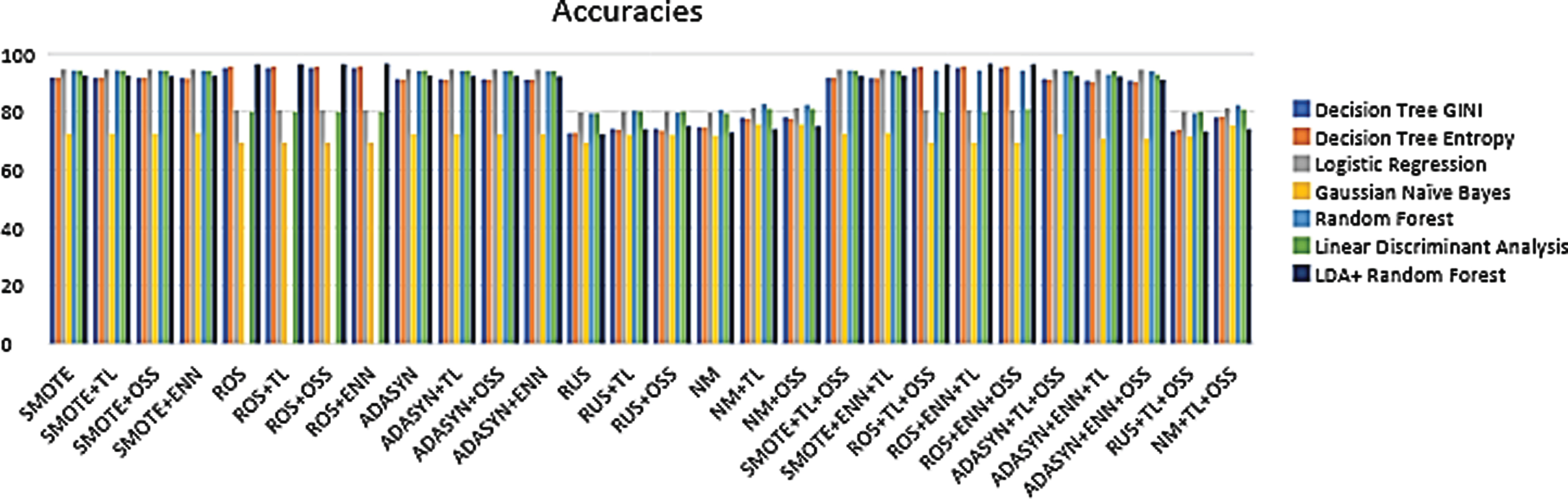
Comparison of accuracies for the patient death dataset.

5.2 Patient health dataset (Pima Indians Diabetes Dataset)

5.2.1 Decision tree using information gain and entropy

Table 17 shows the top 10 variations that were used for this classifier. The highest accuracy obtained here was 75.974% by using Random Oversampler with Tomek Links with the lowest being 64.285% from Adaptive Synthetic Sampler with One Sided Selection and Tomek Links.

Table 17
10 Highest accuracies among 35 in decreasing order

Variation Accuracy Precision Recall F1-Score MCC

ROS+TL 0.83012 0.73 0.80 0.76 0.44

ROS+OSS 0.82257 0.54 0.45 0.48 0.10

ROS+OS+TL 0.82211 0.54 0.45 0.48 0.09

ROS 0.79264 0.70 0.77 0.73 0.38

SMOTE+TL 0.78489 0.69 0.74 0.71 0.38

SMOTE+OSS + TL 0.76016 0.53 0.41 0.45 0.08

SMOTE 0.75860 0.67 0.71 0.69 0.32

ADASY+TL 0.74805 0.68 0.72 0.69 0.34

ADASYN 0.73896 0.63 0.70 0.65 0.29

ADASY+OSS+TL 0.73715 0.51 0.39 0.42 0.08

Variation	Accuracy	Precision	Recall	F1-Score	MCC
ROS+TL	0.83012	0.73	0.80	0.76	0.44
ROS+OSS	0.82257	0.54	0.45	0.48	0.10
ROS+OS+TL	0.82211	0.54	0.45	0.48	0.09
ROS	0.79264	0.70	0.77	0.73	0.38
SMOTE+TL	0.78489	0.69	0.74	0.71	0.38
SMOTE+OSS + TL	0.76016	0.53	0.41	0.45	0.08
SMOTE	0.75860	0.67	0.71	0.69	0.32
ADASY+TL	0.74805	0.68	0.72	0.69	0.34
ADASYN	0.73896	0.63	0.70	0.65	0.29
ADASY+OSS+TL	0.73715	0.51	0.39	0.42	0.08

5.2.2 Decision tree using GINI index

Table 18 shows the top 10 variations that were used for this classifierThe highest accuracy in this classifier was 74.675% by using the Synthetic Minority Oversampler and the lowest resulted from Near Miss at 63.636%.

Table 18
10 Highest accuracies among 35 in decreasing order

Variation Accuracy Precision Recall F1-Score MCC

ROS 0.80658 0.69 0.74 0.71 0.36

ROS+TL 0.79937 0.71 0.77 0.74 0.41

ROS+OSS 0.79787 0.53 0.44 0.48 0.09

ROS+OSS+TL 0.79533 0.53 0.43 0.47 0.08

SMOTE 0.77458 0.69 0.71 0.69 0.35

SMOTE+OSS + TL 0.77376 0.53 0.40 0.45 0.08

SMOTE+OSS 0.76534 0.52 0.40 0.45 0.08

NM+TL 0.76032 0.51 0.39 0.42 0.10

NM+OSS 0.74828 0.52 0.36 0.41 0.10

NM+OSS+TL 0.73932 0.50 0.37 0.42 0.06

Variation	Accuracy	Precision	Recall	F1-Score	MCC
ROS	0.80658	0.69	0.74	0.71	0.36
ROS+TL	0.79937	0.71	0.77	0.74	0.41
ROS+OSS	0.79787	0.53	0.44	0.48	0.09
ROS+OSS+TL	0.79533	0.53	0.43	0.47	0.08
SMOTE	0.77458	0.69	0.71	0.69	0.35
SMOTE+OSS + TL	0.77376	0.53	0.40	0.45	0.08
SMOTE+OSS	0.76534	0.52	0.40	0.45	0.08
NM+TL	0.76032	0.51	0.39	0.42	0.10
NM+OSS	0.74828	0.52	0.36	0.41	0.10
NM+OSS+TL	0.73932	0.50	0.37	0.42	0.06

5.2.3 Logistic regression

Table 19 shows the top 10 variations that were used for this classifier The highest accuracy in this classifier was 72.727% from Synthetic Minority Oversampler with Edited Nearest Neighbors with the lowest being 66.883% from Adaptive Synthetic Sampler with One Sided Selection and Tomek Links.

Table 19
10 Highest accuracies among 35 in decreasing order

Variation Accuracy Precision Recall F1-Score MCC

RUS+OSS+TL 0.77793 0.50 0.37 0.42 0.07

NM+OSS+TL 0.77232 0.50 0.39 0.43 0.07

SMOTE+OSS + TL 0.76847 0.54 0.39 0.45 0.10

SMOTE+TL 0.76777 0.70 0.71 0.69 0.38

SMOTE+OSS 0.76754 0.54 0.40 0.45 0.10

RUS+OSS 0.76669 0.50 0.36 0.40 0.08

RUS+TL 0.76665 0.50 0.36 0.40 0.08

SMOTE 0.76353 0.71 0.72 0.70 0.38

NM+OSS 0.76216 0.51 0.39 0.42 0.09

NM+TL 0.76212 0.50 0.39 0.42 0.08

Variation	Accuracy	Precision	Recall	F1-Score	MCC
RUS+OSS+TL	0.77793	0.50	0.37	0.42	0.07
NM+OSS+TL	0.77232	0.50	0.39	0.43	0.07
SMOTE+OSS + TL	0.76847	0.54	0.39	0.45	0.10
SMOTE+TL	0.76777	0.70	0.71	0.69	0.38
SMOTE+OSS	0.76754	0.54	0.40	0.45	0.10
RUS+OSS	0.76669	0.50	0.36	0.40	0.08
RUS+TL	0.76665	0.50	0.36	0.40	0.08
SMOTE	0.76353	0.71	0.72	0.70	0.38
NM+OSS	0.76216	0.51	0.39	0.42	0.09
NM+TL	0.76212	0.50	0.39	0.42	0.08

5.2.4 Gaussian Naïve Bayes

Table 20 shows the top 10 variations that were used for this classifier. Maximum accuracy in this classifier ranged at 70.779% using Adaptive Synthetic Sampler with One Sided Selection with the minimum being 66.233% by the Random Oversampler.

Table 20
10 Highest accuracies among 35 in decreasing order

Variation Accuracy Precision Recall F1-Score MCC

NM+OSS+TL 0.79298 0.51 0.42 0.45 0.09

NM+OSS 0.78040 0.51 0.42 0.44 0.10

RUS+OSS 0.72257 0.50 0.38 0.42 0.08

RUS+OSS+TL 0.76169 0.50 0.39 0.39 0.07

RUS+TL 0.75253 0.50 0.37 0.42 0.08

SMOTE+OSS 0.74766 0.53 0.37 0.43 0.08

SMOTE+TL 0.74663 0.70 0.67 0.68 0.37

SMOTE+ OSS + TL 0.74552 0.53 0.37 0.44 0.08

NM 0.74440 0.53 0.37 0.44 0.07

SMOTE 0.73844 0.71 0.68 0.68 0.37

Variation	Accuracy	Precision	Recall	F1-Score	MCC
NM+OSS+TL	0.79298	0.51	0.42	0.45	0.09
NM+OSS	0.78040	0.51	0.42	0.44	0.10
RUS+OSS	0.72257	0.50	0.38	0.42	0.08
RUS+OSS+TL	0.76169	0.50	0.39	0.39	0.07
RUS+TL	0.75253	0.50	0.37	0.42	0.08
SMOTE+OSS	0.74766	0.53	0.37	0.43	0.08
SMOTE+TL	0.74663	0.70	0.67	0.68	0.37
SMOTE+ OSS + TL	0.74552	0.53	0.37	0.44	0.08
NM	0.74440	0.53	0.37	0.44	0.07
SMOTE	0.73844	0.71	0.68	0.68	0.37

5.2.5 Random forest

Table 21 shows the top 10 variations that were used for this classifier.The Highest accuracy achieved by this classifier is 74.025% from Synthetic Minority Oversampler using One Sided Selection and the lowest was 62.987% using Near Miss.

Table 21
10 Highest accuracies among 35 in decreasing order

Variation Accuracy Precision Recall F1-Score MCC

ROS+OSS+TL 0.88389 0.55 0.53 0.53 0.12

ROS+OSS 0.87898 0.55 0.49 0.52 0.12

ROS+TL 0.87002 0.79 0.89 0.83 0.54

ROS 0.85279 0.76 0.87 0.81 0.48

SMOTE+OSS 0.83152 0.54 0.44 0.48 0.11

SMOTE+ OSS + TL 0.82898 0.54 0.45 0.48 0.10

SMOTE+TL 0.82431 0.74 0.80 0.77 0.47

ADASYN+TL 0.80804 0.73 0.80 0.75 0.45

SMOTE 0.80766 0.74 0.79 0.44 0.44

ADASYN+OSS+TL 0.80494 0.55 0.44 0.49 0.11

Variation	Accuracy	Precision	Recall	F1-Score	MCC
ROS+OSS+TL	0.88389	0.55	0.53	0.53	0.12
ROS+OSS	0.87898	0.55	0.49	0.52	0.12
ROS+TL	0.87002	0.79	0.89	0.83	0.54
ROS	0.85279	0.76	0.87	0.81	0.48
SMOTE+OSS	0.83152	0.54	0.44	0.48	0.11
SMOTE+ OSS + TL	0.82898	0.54	0.45	0.48	0.10
SMOTE+TL	0.82431	0.74	0.80	0.77	0.47
ADASYN+TL	0.80804	0.73	0.80	0.75	0.45
SMOTE	0.80766	0.74	0.79	0.44	0.44
ADASYN+OSS+TL	0.80494	0.55	0.44	0.49	0.11

5.2.6 Linear discriminant analysis

Table 22 shows the top 10 variations that were used for this classifier. The highest accuracy here was 73.376% by using Synthetic Minority Oversampling with Edited Nearest Neighbors with the lowest from Adaptive Synthetic Sampler with One Sided Selection and Tomek Links at 68.181%.

Table 22
10 Highest accuracies among 35 in decreasing order

Variation Accuracy Precision Recall F1-Score MCC

NM+OSS+TL 0.77653 0.51 0.38 0.42 0.07

RUS+OSS+TL 0.77589 0.50 0.38 0.42 0.07

NM+OSS 0.77236 0.52 0.39 0.43 0.1

RUS+OSS 0.77073 0.50 0.36 0.41 0.08

RUS+TL 0.77069 0.50 0.36 0.40 0.08

NM+TL 0.77028 0.51 0.38 0.42 0.1

ROS+OSS+TL 0.76338 0.54 0.39 0.44 0.1

ROS+TL 0.76025 0.70 0.64 0.7 0.39

ROS+OSS 0.75973 0.53 0.39 0.44 0.09

ROS 0.75852 0.70 0.72 0.70 0.38

Variation	Accuracy	Precision	Recall	F1-Score	MCC
NM+OSS+TL	0.77653	0.51	0.38	0.42	0.07
RUS+OSS+TL	0.77589	0.50	0.38	0.42	0.07
NM+OSS	0.77236	0.52	0.39	0.43	0.1
RUS+OSS	0.77073	0.50	0.36	0.41	0.08
RUS+TL	0.77069	0.50	0.36	0.40	0.08
NM+TL	0.77028	0.51	0.38	0.42	0.1
ROS+OSS+TL	0.76338	0.54	0.39	0.44	0.1
ROS+TL	0.76025	0.70	0.64	0.7	0.39
ROS+OSS	0.75973	0.53	0.39	0.44	0.09
ROS	0.75852	0.70	0.72	0.70	0.38

5.2.7 Linear discriminant analysis+random forest

Table 23 shows the top 10 variations that were used for this classifier. The highest accuracy was 68.831% from Synthetic Minority Oversampler with Edited Nearest Neighbors with lowest at 61.038% from Random Undersampler with Tomek Links.

Table 23
Highest accuracies among 35 in decreasing order

Variation Accuracy Precision Recall F1-Score MCC

ROS+OSS+TL 0.84684 0.54 0.49 0.51 0.09

ROS+TL 0.83431 0.74 0.86 0.79 0.47

ROS 0.83283 0.71 0.86 0.77 0.43

ROS+OSS 0.82470 0.55 0.49 0.52 0.11

SMOTE+ OSS + TL 0.72264 0.53 0.38 0.44 0.09

SMOTE+TL 0.72077 0.55 0.71 0.67 0.33

NM+OSS 0.71955 0.51 0.40 0.43 0.09

NM+TL 0.71951 0.51 0.41 0.44 0.1

RUS+TL 0.71379 0.49 0.36 0.40 0.07

RUS+OSS+TL 0.71262 0.50 0.38 0.41 0.07

Variation	Accuracy	Precision	Recall	F1-Score	MCC
ROS+OSS+TL	0.84684	0.54	0.49	0.51	0.09
ROS+TL	0.83431	0.74	0.86	0.79	0.47
ROS	0.83283	0.71	0.86	0.77	0.43
ROS+OSS	0.82470	0.55	0.49	0.52	0.11
SMOTE+ OSS + TL	0.72264	0.53	0.38	0.44	0.09
SMOTE+TL	0.72077	0.55	0.71	0.67	0.33
NM+OSS	0.71955	0.51	0.40	0.43	0.09
NM+TL	0.71951	0.51	0.41	0.44	0.1
RUS+TL	0.71379	0.49	0.36	0.40	0.07
RUS+OSS+TL	0.71262	0.50	0.38	0.41	0.07

Figure 2 shows accuracy level of each combination of sampling and data reduction method onto multiple classifiers and found that ROS along with TL gives the highest accuracy of 75.97% when applied onto Decision Tree.

Fig. 2

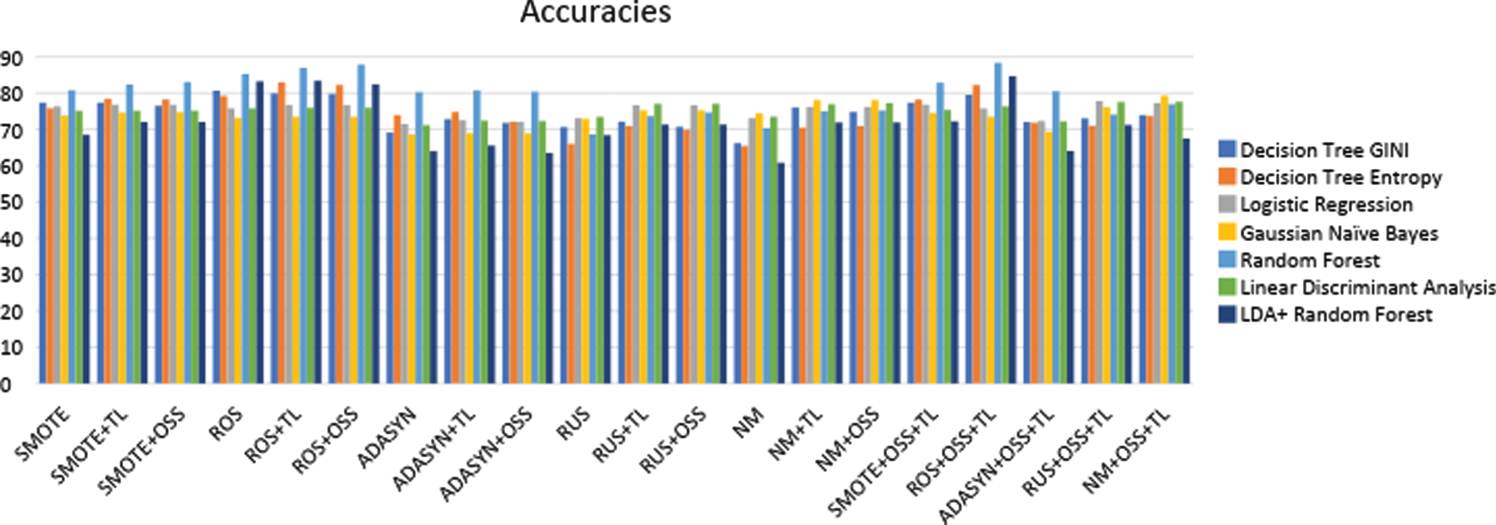
Comparison of accuracies for The Patient Diabetes Dataset.

6 Conclusion

Every step taken in constructing the model has imperative for accurate and precise calculations to obtain the results. If a dataset is not properly balanced, the minority class can be ignored by the algorithms and give an unfair result which is completely biased. That needs to be fixed when classifying the data.

In our work, we have experimented with two imbalanced datasets which varies in size in terms of number of instances.. One was highly complex and of a humongous level with 187 features and having over 90000 samples in total being considered for the predictions which was the patient death dataset and the other was completely opposite having just about 9 features for consideration and approximately 800 samples in total which was the diabetes dataset.

These highly variable datasets were chosen deliberately to observe the impact of sampling technique along with classifier performance. Further, for analyzing the performance seven classifiers were used. Instead of using raw data,we have focused on balancing the imbalanced dataset. For the same, three oversampling methods (SMOT, ROS and ADASYN) and two undersampling methods (RUS and Near Miss) were experimented. Extension of these sampling methods was also experimented by pairing the same with data cleaning and reduction methods (TL,ENN,OSS) and this has shown a significant improvement.

At last, we found that combination of ADASYN along with OSS perform better in case of large size dataset while combination of ROS along with TL showed better performance in case of low size data dataset. We have also analyzed that oversampling technique gives quite promising results in comparison to undersampling methods specifically when applied with machine learning classifiers.

References

Krawczyk and sBartosz, Learning from imbalanced data: Open challenges and future directions, Progress in Artificial Intelligence 5 (2016), 10.1007/s13748-016-0094-0.

Provost

, Machine learning from imbalanced data sets 101, In Proceedings of the AAAI’2000 workshop on imbalanced data sets 68 (2000), 1–3. AAAI Press.

Elhassan

and Aljurf

, Classification of imbalance data using tomek link (t-link) combined with random undersampling (rus) as a data reduction method, 2016.

Hawkins

D.M.

, The problem of overfitting, Journal of Chemical Information and Computer Sciences 44(1) (2004), 1–12.4.

Chawla

N.V.

, Bowyer

K.W.

, Hall

L.O.

and Kegelmeyer

W.P.

, SMOTE: synthetic minority over-sampling technique, Journal of Artificial Intelligence Research 16 (2002), 321–357.

Kotsiantis

, Kanellopoulos

and Pintelas

, Handling imbalanced datasets: A review, GESTS International Transactions on Computer Science and Engineering 30(1) (2006), 25–36.

Maestre-García

F.J.

, García-Martínez

, Pérez-Ortiz

and Gutiérrez

P.A.

, An Iterated Greedy Algorithm for Improving the Generation of Synthetic Patterns in Imbalanced Learning. In International Work-Conference on Artificial Neural Networks (2017), pp. 513–524. Springer, Cham.

Rahman

M.M.

and Davis

D.N.

, Addressing the class imbalance problem in medical datasets, International Journal of Machine Learning and Computing 3(2) (2013), 224.

and Lee

J.S.

, A new under-sampling method using genetic algorithm for imbalanced data classification. In Proceedings of the 10th International Conference on Ubiquitous Information Management and Communication (2016), 1–6.

10.

Suman

, Laddhad

and Deshmukh

, Methods for handling highly skewed datasets. Part I-October, 3. 2005.

11.

Kubat

and Matwin

, Addressing the curse of imbalanced training sets: one-sided selection, In Icml 97 (1997), 179–186.

12.

Raniszewski

, The edited nearest neighbor rule based on the reduced reference set and the consistency criterion, Biocybernetics and Biomedical Engineering 30(1) (2010), 31–40.

13.

Boughorbel

, Jarray , Fethi and El-Anbari , Mohammed, Optimal classifier for imbalanced data using Matthews Correlation Coefficient metric, PLOS ONE 12 (2017), e0177678. 10.1371/journal.pone.0177678.

14.

Fernández Hilario

A.L.

, García López

, Herrera Triguero

and Chawla

N.V.

, SMOTE for Learning from Imbalanced Data: Progress and Challenges, Marking the 15-year Anniversary, 2018.

15.

Lemaître

, Nogueira

and Aridas

C.K.

, Imbalanced-learn: Apython toolbox to tackle the curse of imbalanced datasets in machine learning, The Journal of Machine Learning Research 18(1) (2017), 559–563.

16.

Hssina

, Merbouha

, Ezzikouri

and Erritali

, A comparative study of decision tree ID3 and C4. 5, International Journal of Advanced Computer Science and Applications 4(2) (2014), 13–19.

17.

Suneetha

, Hari

and Kumar

V.S.

, Modified gini indexclassification: a case study of heart disease dataset, International Journal on Computer Science and Engineering 2(06) (2010), 1959–1965.

18.

Korkmaz

, GÜNEY

and YİĞİTER

Ş.

, Theimportance of logistic regression implementations in the Turkish livestock sector and logistic regression implementations/fields, Harran Tarım ve Gıda Bilimleri Dergisi 16(2) (2012), 25–36.

19.

Murphy

K.P.

, Naive bayes classifiers, University of British Columbia 18 (2006), 60.

20.

Biau

, Analysis of a random forests model, Journal of Machine Learning Research 13(Apr) (1063), 1095.

21.

Torkkola

, Linear discriminant analysis in document classification. In IEEE ICDMWorkshop on Text Mining (2001), 800–806.

22.

Data set Patient Health dataset: https://www.kaggle.com/c/widsdatathon/data

23.

Pima Indians Diabetes Dataset: https://www.kaggle.com/uciml/pima-indians-diabetes-database

24.

Padurariu

and Breaban

M.E.

, Dealing with data imbalance in text classification, Procedia Computer Science 159 (2019), 736–745.

25.

Scholkopft

and Mullert

K.R.

, Fisher discriminant analysis with kernels, Neural Networks for Signal Processing IX 1(1) (1999), 1.

26.

Denil

, Matheson

and De Freitas

, January. Narrowing the gap: Random forests in theory and in practice. In International Conference on Machine Learning (2014), 665–673.

27.

Salmi

and Rustam

, Naïve Bayes Classifier Models for Predicting the Colon Cancer, In IOP Conference Series:Materials Science and Engineering 546(5) (2019), 052068. IOP Publishing.

28.

Park

, An introduction to logistic regression: from basic concepts to interpretation with particular attention to nursing domain, Journal of Korean Academy of Nursing 43(2) (2013), 154–164.

29.

Brijain

, Patel

, Kushik

and Rana

, A survey on decision tree algorithm for classification, 2014.

30.

and Claramunt

, A spatial entropy-based decision tree for classification of geographical information, Transactions in GIS 10(3) (2006), 451–467.

31.

Yung

, Brown

E.T.

, Rasin

, Furst

J.D.

and Raicu

D.S.

, Synthetic Sampling for Multi-Class Malignancy Prediction. arXiv preprint arXiv:1807.02608, 2018.

32.

Agrawal

, Viktor

H.L.

, Paquet

and SCUT:

November.

, Multi-class imbalanced data classification using SMOTE and cluster-based undersampling, In 2015 7th International Joint Conference on Knowledge Discovery, Knowledge Engineering and Knowledge Management (IC3K) 1 (2015), 226–234. IEEE.

33.

Batista

G.E.

, Prati

R.C.

and Monard

M.C.

, A study of the behavior of several methods for balancing machine learning training data, ACM SIGKDD Explorations Newsletter 6(1) (2004), 20–29.

34.

Yen

S.J.

and Lee

Y.S.

, Under-sampling approaches for improving prediction of the minority class in an imbalanced dataset. In Intelligent Control and Automation (2006) (pp. 731–740). Springer, Berlin, Heidelberg.

35.

Guan

, Yuan

, Lee

Y.K.

and Lee

, Nearest neighbor editing aided by unlabeled data, Information Sciences 179(13) (2009), 2273–2282.

Classification of imbalanced medical data: An empirical study of machine learning approaches

Abstract

Keywords

1 Introduction

Table 1 List of abbreviations Abbreviation Full Form SMOTE Synthetic Minority Oversampling Technique ADASYN Adaptive Synthetic Sampler ROS Random Oversampler RUS Random Undersampler TL Tomek Links OSS One Sided Selection ENN Edited Nearest Neighbors

2.1 Sampling based methods

2.3 Classification techniques

2.3.1 Decision tree using information gain and entropy

2.3.6 Linear discriminant analysis

3 Methodology

3.1 Data Preparation and pre-processing

3.2 Data Resampling and further utilization

3.3 Standardization

3.5 Performance and evaluation measures

Table 2 Composition of the dataset Count Number of Instances Count of ‘0’ 83798 Count of ‘1’ (Deaths) 7915

4.1.1 Data resampling techniques

4.1.2 Classifiers

4.1.3 Data reduction techniques

5 Results

5.1 Patient health dataset (Death)

5.1.1 Decision tree using information gain and entropy

5.2.1 Decision tree using information gain and entropy

References

Table 1
List of abbreviations

Abbreviation Full Form

SMOTE Synthetic Minority Oversampling Technique

ADASYN Adaptive Synthetic Sampler

ROS Random Oversampler

RUS Random Undersampler

TL Tomek Links

OSS One Sided Selection

ENN Edited Nearest Neighbors

Table 2
Composition of the dataset

Count Number of Instances

Count of ‘0’ 83798

Count of ‘1’ (Deaths) 7915