




Abstract
In the present study, three hybrid models include support vector regression-salp swarm optimization (SVR-SSO), support vector regression-biogeography-based (SVR-BBO), and support vector regression-phasor particle swarm optimization (SVR- PPSO) was applied to forecast pond ash’s CBR value modified with lime sludge (LS) and lime (LI). In the developed models, five variables were selected as inputs. It can result that the developed integrated models have R2 bigger than 0.9952. It means the agreement between observed and forecasted values by hybrid models is mainly similar to represent the highest accuracy. In both the training and testing stages, PSO-SVR results from better performance than the BBO-SVR model, with R2, RMSE, MAE, and PI equal to 0.9983, 0.6439, 0.3181, and 0.0081 for training data, and 0.9975, 0.7319, 0.4135, and 0.0141 for testing data, respectively. So, by considering the OBJ index, the OBJ value for PSO-SVR is 12.966, lower than BBO-SVR at 16.9957. Therefore, the PSO-SVR model outperforms another model to estimate the CBR of pond ash modified with LI and LS, consequently being recognized as the proposed model that makes it to be used for practical applications.
Keywords
Introduction
Thermal power plants produce various ashes, such as fly ash and pond ash [1, 2]. Bottom ash generated from the boiler and fly ash produced from the electrostatic precipitators is blended with water and produced slurry and disposed of in ash ponds [3]. Fly ash type C has a large calcium content level and could react with water [4]. Other ashes are class F with low calcium and great thermal power plant [5]. This type of ash does not have sufficient strength to be used as an independent construction component. This ash’s deficiency could be improved by other cementitious materials like lime and cement, which were evaluated by several studies [6–9]. The production of acetylene, sugar, and water softening plants is lime sludge as another material. Annually, about 4.5 million tons of lime sludge is produced in India [10], causes disposal, and alters into a worrying environmental matter [11–13]. Due to this material containing calcium carbonate [14], it can be used in several construction fields, like a substitution of cement [10], in the road [15], and in construction materials [16].
California bearing ratio (CBR) is a superior parameter to appraise the soil subgrade, either flexible or rigid pavements [17]. CBR test is performed on compacted samples of soil in the lab and is performed on the ground [18]. Besides CBR being the time needed, the test conclusion can be untrustable due to the specimen disturbance and restrictions of testing circumstances. Thus, artificial-based techniques can be efficient in the various forecasting procedures [19], particularly CBR [20].
Pavement subgrade soils were modified by different waste marble powders: 1) calcite marble and 2) dolomitic marble powder. California bearing ratio was provided to compute the improvement in capacity. According to the comparison based on the values of CBR, the inclusion of an appropriate amount and kind of marble powder positively affected the bearing capacity of the subgrade soil with no regard to the curing time [21, 22].
Regarding artificial intelligence methods, the neural network (NN) is a human brain simulation and was extensively agreed in various branches to illustrate the connections between inputs and output. Thus, the neural network is an adequately accurate solution for predicting the most geotechnical engineering field. The neural network has been effectively applied in different branches of geotechnical engineering, such as the CS and the frozen sand of Young’s modulus [23, 24], bearing capacity of the pile [25, 26], stability of slope [27–29], and underground structures [30, 31].
In spite of several NN applications being created in geotechnical engineering, research for predicting the CBR is low. Single and multiple analyses were employed for forecasting the CBR value by a dataset collected from highways of Turkey located in different regions. The conclusion presents that the NN has appropriate results compared to statistical models [32]. The neural network and multiple regression methods were used for forecasting the CBR value of modified soil with admixtures such as lime and quarry [33]. Both proposed models predicted the CBR precisely, while the neural network outperforms multiple regression. Two modeling methods, named random forest and M5P-Tree models, are applied for modeling the soaked CBR value of pond ash. Pond ash was stabilized with the help of additives like lime and lime sludge. Standard statistical parameters estimated the performance of models. Despite both of the model’s performance for predicting CBR is good enough, it is explicit which the random forest technique outperforms the M5P model [34].
For dealing with real-world challenges related to HPC, machine learning techniques have proven to be effective. Noteworthy methods include the artificial neural network (ANN), gene expression programming (GEP), support vector machine (SVM), multi-layer perceptron neural network (MLP), and the multigroup approach for data management. These techniques have been utilized to predict the desired output data in the context of HPC. In recent years, machine learning approaches have demonstrated significant promise in predicting concrete strength. Support Vector Regression (SVR) [35] has risen as an efficient and robust method among these techniques for modeling and predicting complex nonlinear relationships. The successful application of SVR in various fields can be attributed to its capability to effectively deal with nonlinearity, reduce the risk of overfitting, and handle high-dimensional data [36].
Despite SVR demonstrating promising results, the optimization of its parameters is essential to further improve its predictive performance [35]. With this objective in mind, researchers have investigated the incorporation of diverse optimization algorithms to enhance the accuracy and convergence speed of the SVR model. In this paper, biogeography-based optimizer (BBO), phasor particle swarm optimization (PPSO), and salp swarm optimization (SSO) have emerged as effective optimizers in different domains.
Lately, the application of geosynthetic stabilized soil has become popular to construct tolerable pavement structures. The CBR evaluates its resistance. The study’s main aim was to figure out and assess the competency of various techniques, for instance, ANN, M5 model trees, and random forests, to estimate the CBR of modified soil [37].
In the present study, two hybrids, biogeography-based support vector regression (BBO-SVR) and particle swarm optimization-support vector regression (PSO-SVR), were applied to forecast pond ash’s CBR value. To aim goal, the developed models include five inputs named MDD, OMC, L, LS, and CP, and CBR as a target parameter. So as to appraise the precision of the proposed models, five performance criteria (R2, RMSE, MAE, PI, and OBJ) were considered.
Methodologies
Dataset explanation
To train the proposed models for predicting the CBR value, a dataset comprising 109 experimental measurements was collected from published documents (refer to Table 1) [38]. Eight different influencing variables to the value of output were taken into account as input parameters. The statistical explanation of the dependent and independent parameters utilized for proposing the integrated models is supplied in Table 2. Fig. 1 presents a multi-Y scatter plot illustrating the connection between the input and output variables, visually depicting their interrelation.
Mix designs and CBR results
Mix designs and CBR results
Liquid limit (LL), plastic limit (PL), Plasticity Index (PI), optimum moisture content (OMC) and maximum dry density (MDD), Soil Dispersibility Index (SDA), Quality Deficiency (QD), Ordinary Portland Cement (OPC), California Bearing Ratio (CBR).
The statistical description of the dependent and independent variables
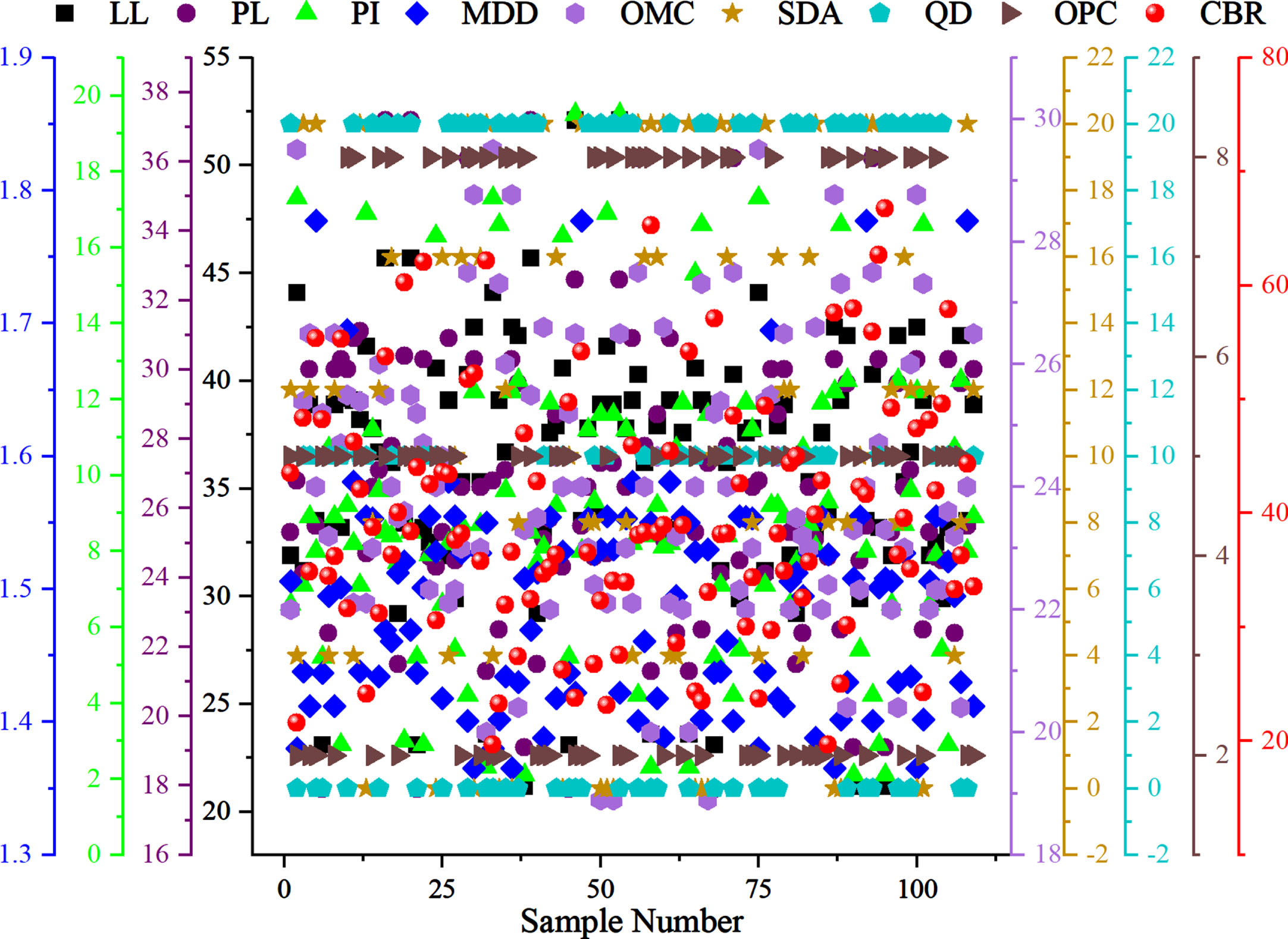
The scatter of input and output variables.
Support vector machines are regression and classification models derived from statistical learning theory. The Support vector machines-based classification methods are based on the generality of the best separation of classes. If the classes are separable –this method selects, from among the unlimited number of linear classifiers, the one that minimizes the generalization error, or at least an upper bound on this error, derived from structural risk minimization. SVR has additive advantages when compared to other regression methods [39, 40]. Considering a training dataset { (x i , y i ) , I = 1, … n }, where n is the size of the training dataset, (x i ) is the input vector (y i ) is the output vector, respectively.
Minimizing the Euclidean norm leads to a smaller value of m, indicating the flatter nature of Equation (1) defined by ∥
Equation (2) assumes that there exists an expansion that can generate an error smaller than ɛ for all training pairs. However, in real-world scenarios, there may be situations, such as those encountered in classification problems, that do not conform to this assumption.so that’s why, to allow some more error, slack variables ξ, ξ can be optimized and to handle the infeasible constraints of the optimization problem defined in Equation (3), the following approach can be employed [41].
The constant G > 0 is a parameter of user-defined which determines the trade-off between function flatness. Equation (3) defines the objective primal function in the minimization problem [42]. By transforming the problem into a dual space representation using Lagrangian multipliers, the inequalities can be replaced with a simpler form, allowing the optimization problem to be solved more easily. Equation (5) the lagrangian can be formed by introducing positive multipliers
In Equation (6), the dual variables have to suffice
Results of substituting Equations (7)–(10) in Equation (6) in the optimization problem of maximizing:
In Equations (9) and (10) dual variables
In Equation (7), the regression problem in feature space can be written by replacing
In Equation (8), the function of SVR can now be written as:
Finally, the kernel function. In this optimization problem, it is computed rather than
The parameter’s setting
By leveraging the advancements in PSO algorithms demonstrated in previous research, it becomes possible to regulate and guide a system or process by employing suitable control methods. To optimize a given problem successfully, the parameters of Particle Swarm Optimization (PSO) need to incorporate various strategies. The primary objective of this study is to improve the convergence capability during the optimization process by enhancing the effectiveness of optimization. To achieve these goals, the PPSO utilizes appropriate and efficient phasor angle functions to generate control parameters for PSO. Each particle is assigned an individual scalar phasor angle to implement a range of strategies effectively. Mathematical functions involving both cosine and sine are employed to model the PSO control parameters based on these phasor angles. As an illustration, it is noted that the ith particle is denoted by
Like the PSO - TVAC in [44] and a modern PSO - TVAC [45], the inertia weight values of PPSO is considered zero. The proposed model for particle movement in PPSO is outlined below. However, it is possible to enhance this method by incorporating concepts from other improved PSO algorithms.
The PPSO algorithm has chosen the following functions after analyzing a large number of
The functions proposed in this study, relying solely on the phasor angles of the particles, exhibit various behaviors, including value reversal, simultaneous increase or decrease of values, reaching large values, and attaining identical values. These behaviors contribute to adaptive search characteristics, balancing local and global searches. As a result, PPSO stands out as an adaptive and non-parametric algorithm capable of avoiding local optima and mitigating premature convergence, a drawback frequently observed in traditional PSO approaches.
In each iteration of the algorithm, the velocity of individual particles is calculated using the following formula.
Subsequently, the particle’s position is updated utilizing the following equation:
Following that, the determination of the Personal Best (P best ) and Global Best (G best ) positions follow a process similar to the conventional PSO algorithm. Afterward, the phasor angles and maximum velocities of the particles undergo an update according to the following procedure:
It is worth noting that Equations (18) to (20) and (23) to (24) are based on empirical formulas that were chosen after testing a vast array of functions. The number of functions assessed for this purpose was substantial, and it is not feasible to present all of them here. Figure 2 displays the flowchart of PPSO.
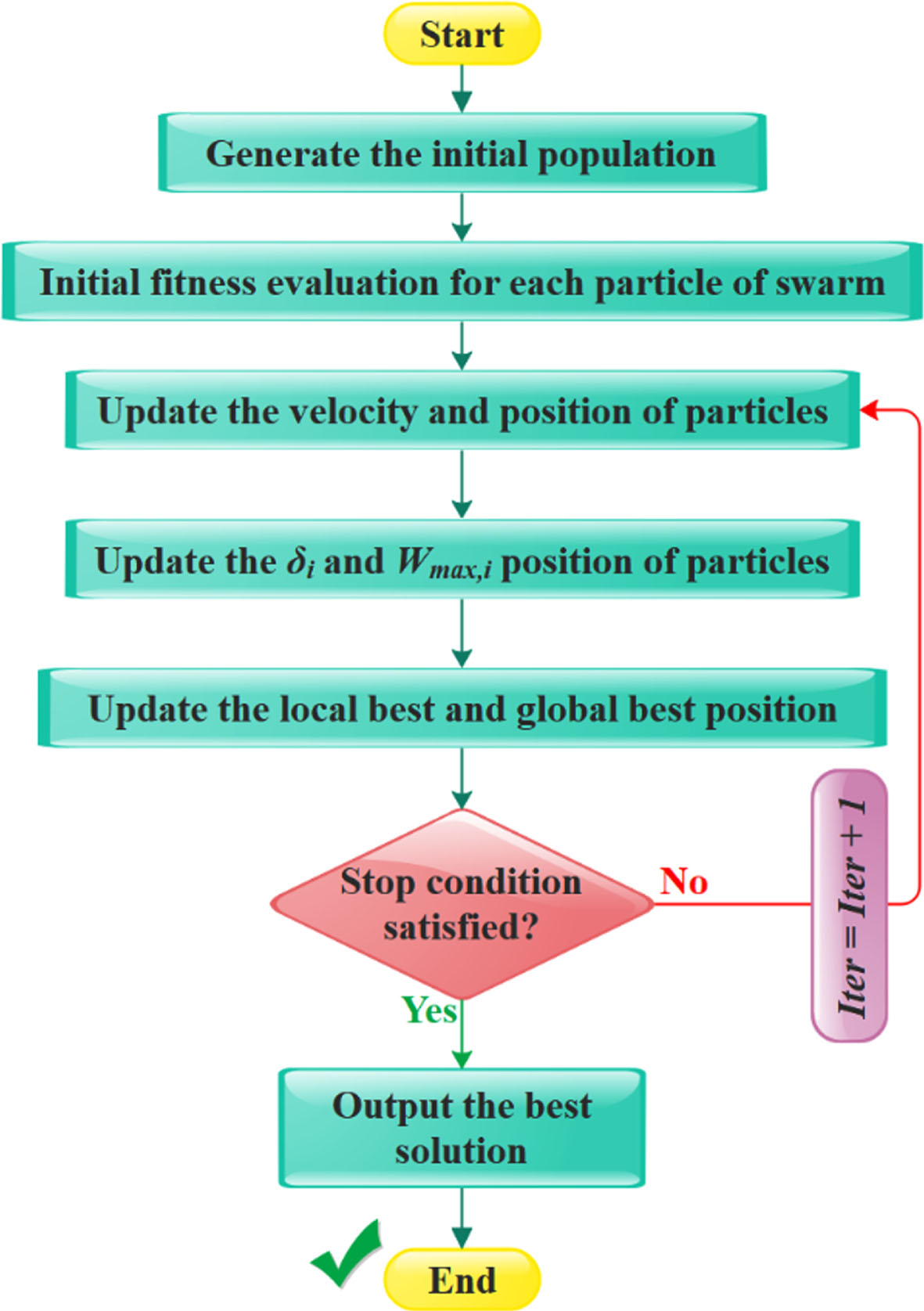
Flowchart of PPSO.
This subsection presents an overview of the biogeography-based optimization algorithm. Imagine there is an optimization problem along with a set of candidate solutions. In this context, a favorable solution can be compared to a habitat with a high habitat suitability index (HSI), analogous to a geographical area well-suited for biological species in biogeography. Within the optimization problem, the HSI serves as a measure of the solution’s quality, often referred to as fitness or goodness of the habitat [46]. Conversely, a subpar solution resembles a habitat with a low HSI. High Habitat Suitability Index (HSI) in solutions indicates habitats that support a diverse array of species, whereas low HSI solutions signify habitats with fewer species. In essence, the number of species represented by a solution depends on its corresponding HSI. Solutions with high HSI are more likely to share their characteristics with other solutions, while solutions with low HSI are more inclined to accept shared attributes from other solutions. This novel approach to address general optimization problems is biogeography-based optimization (BBO). Like other evolutionary algorithms, BBO relies on two crucial steps: information sharing, achieved through migration in BBO, and mutation. Migration, as a probabilistic operator, enhances a habitat, denoted as H i . The migration rates of each habitat are utilized to probabilistically share features among habitats. For every habitat H i , its immigration rate, K i , is employed to determine probabilistically whether it should undergo immigration [47]. If immigration is chosen, then the emigrating habitat, H j , is also selected probabilistically based on the emigration rate, l j . In this context, migration is defined as the process by which features are exchanged between habitats to improve their overall optimization performance.
In the field of biogeography, an SIV, known as a Suitability Index Variable, plays a crucial role in assessing an island’s livability. Within the context of BBO an SIV represents a characteristic of a solution, analogous to a gene in GAs. Mutation serves as a probabilistic operator responsible for randomly altering an island’s SIV, relying on the pre-existing probability of species count in that habitat [48, 49]. Mutation serves the primary objective of promoting diversity within the population. In the case of low HSI solutions, mutation offers an opportunity to enhance the quality of these solutions. Conversely, for high HSI solutions, mutation can further improve them beyond their current state. The pseudocode for BBO′s migration operator is depicted in Algorithm 1.
SSO [50] is a novel optimization technique that addresses diverse optimization problems. This method emulates the movement of salps, barrel-shaped plankton belonging to the Salp family, found in the wild. Salps share similarities with jellyfish in terms of their tissue structure, and their movement is primarily driven by the expulsion and contraction of water within their gel-like bodies, which have a high water content. By imitating this natural behavior, the optimization method finds solutions efficiently for various optimization challenges [51, 52]. The marine salp exhibits a herding behavior known as the salp chain, which aids them in inefficient movement and feeding by adapting swiftly to changes in their environment. Drawing inspiration from this behavior, the algorithm has mathematically modeled and applied the Salp chain to test its effectiveness in solving an optimization problem.
SSO initiates by segregating the population into two categories: leaders and followers. The rest of the salps are referred to as followers, while the salp preceding them in the sequence assumes the role of the leader. The salp’s position is determined in an n-dimensional space, representing the search space of the problem, with n denoting the number of variables under consideration. These salps diligently search for food sources, which indicate the direction of the entire herd’s destination. To frequently update the location of the Salp leader, the following formula is employed for this purpose:
Here
Here l max and l show the maximum number of iterations and the current repetition, respectively. Once the leader’s position has been updated, SSA proceeds to update the position of the followers using the following formula:
The pseudocode for the SSA algorithm is illustrated in Algorithm 2.
In machine learning models, hybridization involves amalgamating various algorithms, techniques, or approaches to form a cohesive, unified model. The purpose of hybridization is to capitalize on the unique strengths of each component, resulting in improved overall performance, accuracy, or efficiency compared to using any single method in isolation. Hybridizing Support Vector Regression (SVR) with different optimization algorithms can potentially lead to improved performance and model robustness. In all three cases, the primary objective is to find the best hyperparameters for the SVR model to achieve better generalization and performance on the given dataset. By leveraging the strengths of each optimization algorithm, the hybridized approach can potentially enhance the model’s ability to handle complex relationships and improve its overall accuracy. However, it is essential to conduct thorough experimentation and fine-tuning to ensure the hybridized model’s optimal configuration. To enhance comprehension of the procedure utilized in this study, Fig. 3 has been provided.
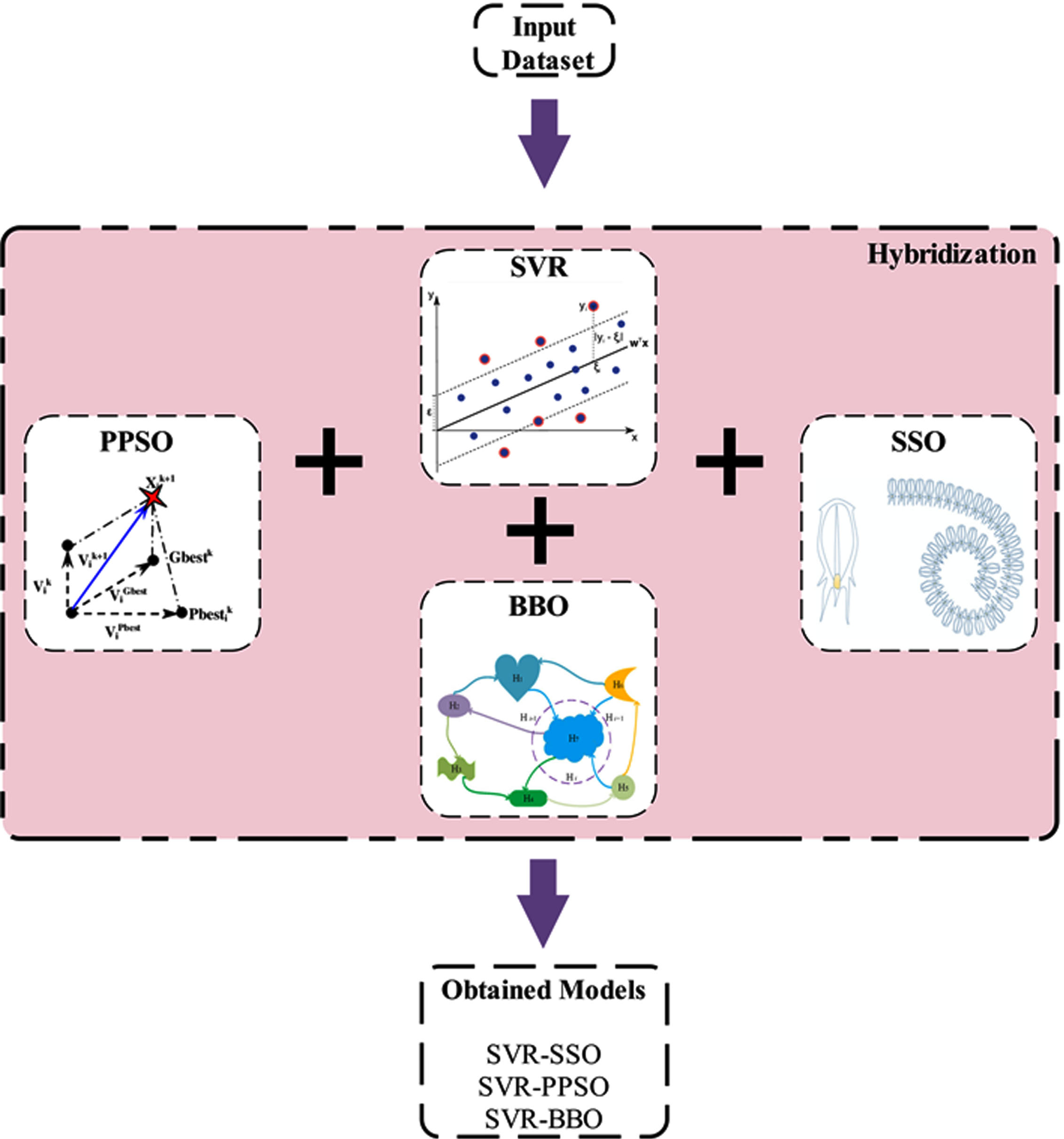
The process of Hybridization.
Various appraisals were utilized to evaluate the workability of models for forecasting the CBR value. Coefficient of determination (R2), root mean squared error (RMSE), mean absolute percentage error (MAPE), mean absolute error (MAE), performance index (PI), and OBJ (Equations (29)–(33)):
Convergence curve analysis
Figure 4 illustrates the convergence curve of the proposed machine learning models, also known as a learning curve, indicating how model performance evolves or stabilizes with increasing training data. The y-axis represents the RMSE, while the x-axis displays the number of iterations. Analyzing this curve provides valuable insights into the model’s learning behavior and facilitates data-driven decisions concerning the need for additional training data or whether the model has reached its optimal performance. The initial iterations demonstrate the steepness of the models’ learning, and some overlap exists among the models. However, beyond the 90th iteration, all models attain their optimal results. Remarkably, SVR-SSO stands out with its superior performance relative to the other models, as evident from the results.
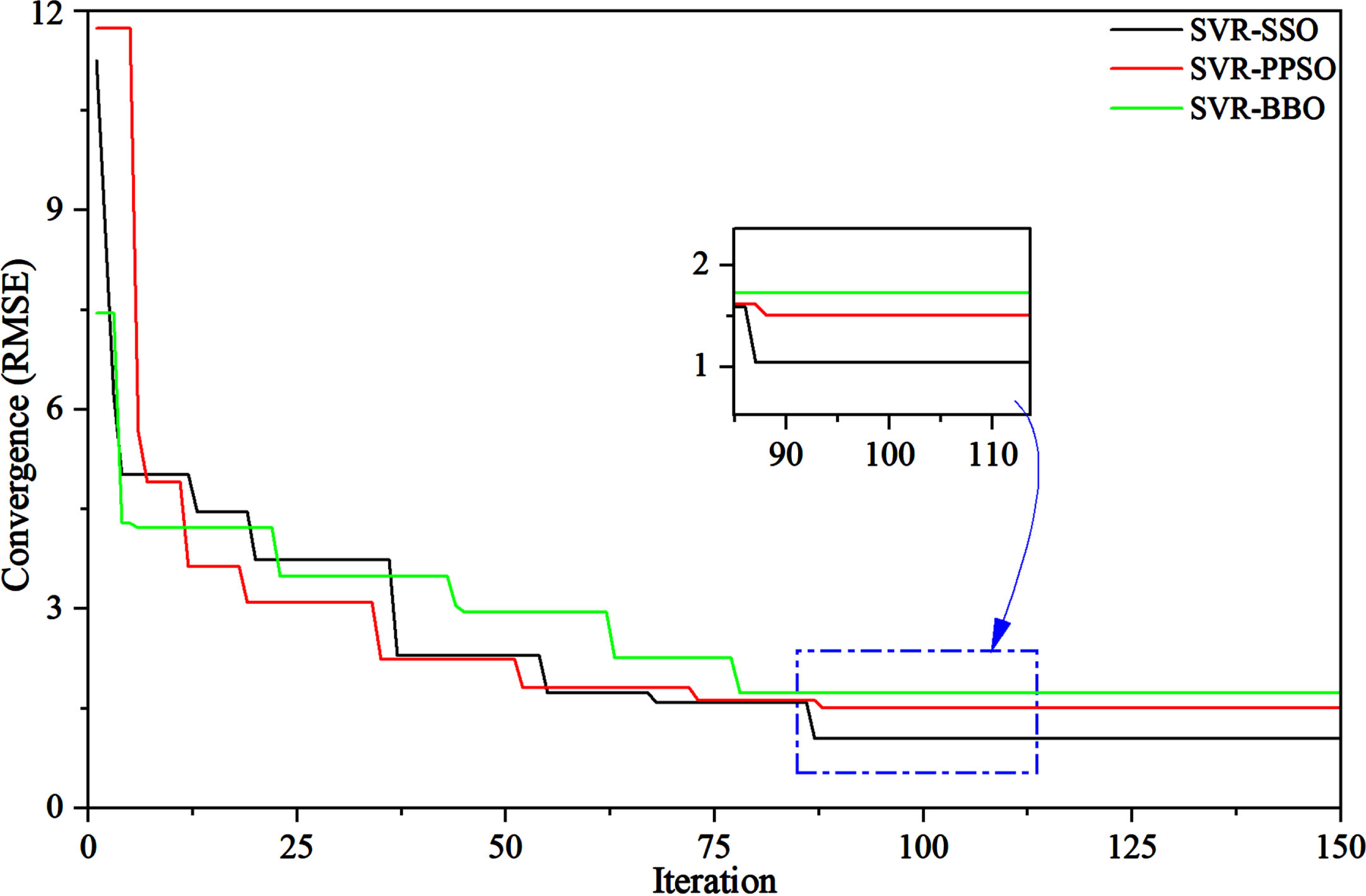
The convergence curve for the presented hybrid models.
This section presents the results of training the admixture inputs of the CBR using machine learning methods. The classical SVR model achieved acceptable results but with a lack of accuracy. Hybridization techniques were employed to address this, utilizing PPSO, BBO, and SSO to enhance the SVR model’s performance. The proposed hybrid models are denoted as SVR-PPSO, SVR-BBO, and SVR-SSO. The evaluation of these models is carried out in two stages: training and testing. The dataset consists of a total of 109 CBR samples, which are utilized in both stages. More specifically, 70% of the data is allocated for training, while the remaining 30% is used for testing. To ensure unbiased and robust model performance comparisons, various performance evaluators, including R2, RMSE, MAE, PI, and OBJ, were utilized. These evaluators provide a comprehensive assessment of the models and enable a thorough evaluation of their effectiveness. In the context of the evaluators, a high R2 value approaching 1 indicates an optimal result, while low values for RMSE, MAR, PI, and OBJ, approaching 0, indicate an optimal outcome. Table 3 presents the mentioned models’ results and their corresponding metrics. A rank score ranging from 1 to 4 has been provided to facilitate a more effective comparison of the models. The highest accuracy result for each metric is assigned rank 4, while the least accurate results are assigned rank 1.
The results of created models for predicting CBR
The results of created models for predicting CBR
As shown in Table 3, the results clearly indicate the SVR single form’s lack of accuracy compared to the other models, as evidenced by its RMSE value of 2.172 in the training phase and 2.604 in the testing phase. However, when applying optimizers to SVR, a significant improvement of at least 20% in its lowest RMSE is observed, demonstrating the effectiveness of the applied optimizers. The SVR-SSO model achieved the highest accuracy among all the other models, demonstrated by the highest R2 value and the lowest error indicators. Notably, the SVR-SSO model’s accuracy further improved during the testing phase compared to its performance during the training phase. These results underscore the model’s effectiveness in predicting CBR values with precision. However, despite the improvement observed in the other two hybrid models compared to the single form of SVR, their accuracy still falls short of the SVR-SSO model. The SVR-SSO model outperforms the SVR-PPSO model by 45% and the SVR-BBO model by 58% in terms of the lowest RMSE.
Figure 5 presents a scatter plot illustrating the correlation between the measured and predicted values of the proposed hybrid models, allowing for an assessment of their accuracy. The plot differentiates the values from the train and test phases using distinct colored squares scattered around a center line that represents an R2 value of 1. The y-axis represents the measured values, while the x-axis represents the predicted values. In an ideal scenario, the majority of train and test values are closely aligned with the center line, indicating the accuracy of the models. The proximity of the scattered points to the center line suggests that the predictions are in good agreement with the actual measurements, and the models’ performance is noteworthy. Upon observing the SVR-SSO scatter plot, it becomes evident that the test phase values are almost perfectly aligned with the center line, indicating an excellent correlation between the predicted and measured values. Furthermore, the training phase values show a maximum level of correlation with the center line, signifying the model’s strong performance in accurately predicting both the training and test data points. The proximity of the scattered points to the center line in both phases demonstrates the remarkable accuracy and effectiveness of the SVR-SSO model in this analysis. However, both the SVR-PPSO and SVR-BBO models exhibit similar behavior in their performance, with their data showing an acceptable dispersion around the center line. While they do not achieve the same level of perfect alignment as the SVR-SSO model, the scattered points for both SVR-PPSO and SVR-BBO remain close to the center line. This indicates a reasonable correlation between the predicted and measured values for both training and test phases. Though not as accurate as the SVR-SSO model, the SVR-PPSO and SVR-BBO models still demonstrate commendable performance in their predictions, making them valuable alternatives in this analysis.
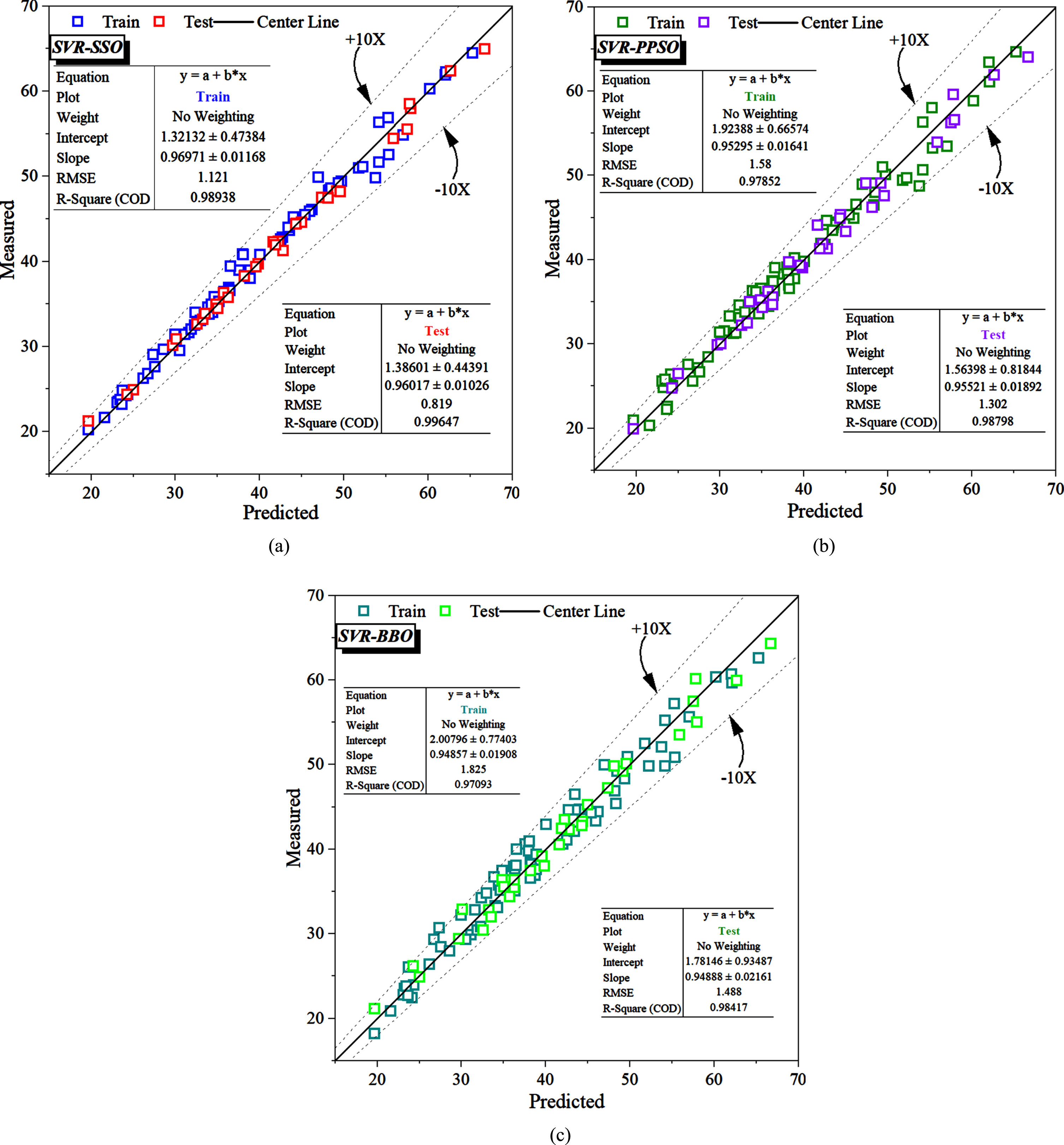
The scatter plot for the correlation between predicted and measured CBR.
The line-symbol plot in Fig. 6 offers a visually detailed representation of the correlation between the measured and predicted values of the hybrid models. The measured values are depicted by a black line, and the alignment of the train and test values with this line indicates the accuracy of the models. By using this plot, it becomes evident how closely the train and test values align with the measured value line, allowing for a quick assessment of each model’s accuracy. The clarity of the plot aids in visualizing the performance of the hybrid models and provides valuable insights into the quality of their predictions.

The line-symbol plot for the comparison between predicted and measured CBR.

The error percentage for the column plot of developed models.
To better visualize the models’ performance, Figs. 7 and 8 have been provided to indicate the errors of the models. As evident from the figures, the majority of SVR-SSO data values are below 5 percent error, with a maximum error of 7.74% occurring between sample numbers 30 to 40. Figure 7 reinforces the low error percentage, with the majority of data points having errors close to 0 and distributed below 5% error.

The scatter interval plot for the error percentage of presented models.
However, SVR-PPSO and SVR-BBO exhibit higher error rates of 10.5% and 11.79%, respectively, both occurring in the training phase. This is evident when observing their error balance, ranging between -10 to 10, and the distribution of errors is more pronounced in Fig. 7. In contrast, the error distribution of SVR-BBO exhibits a notably flatter normal distribution in comparison to alternative models, as discernible from Fig. 8. The distribution of errors in SVR-BBO, as visually represented in Fig. 8, is distinguishably flatter when compared to other models. Conversely, SVR-SSO demonstrates a higher concentration of data points near zero percent, indicative of heightened model precision and a distinctively sharper normal distribution. This observation underscores the superiority of SVR-SSO in terms of predictive accuracy and model performance, as evidenced by the distribution characteristics displayed in Fig. 8. Such nuanced distinctions within the error distributions, as portrayed in Fig. 8, shed light on the efficacy of different optimization strategies when applied to support vector regression.
Figure 9 illustrates a Taylor diagram comparing CBR’s predicted and measured values. The Taylor diagram serves as a valuable tool for evaluating the performance of multiple models in relation to a reference dataset, which, in this case, is the CBR value. In Fig. 9, the correlation coefficient is represented on a scale from -1 to 1, indicating the extent of agreement or disagreement between the model predictions and the observed CBR values. A correlation coefficient of 1 denotes a perfect match, while -1 indicates a perfect inverse relationship. Additionally, the standard deviation is depicted on a scale from 0 to 15, signifying the variability of the model predictions in comparison to the measured CBR values. A lower standard deviation indicates greater consistency and agreement between the models and the reference dataset. In Fig. 9, the green, pink, and blue dots represent the SVR-SSO, SVR-PPSO, and SVR-BBO models, respectively. Upon analyzing the diagram, it becomes evident that the SVR-SSO model is the closest to the reference point, indicating a suitable match with the target. Both SVR-BBO and SVR-PPSO demonstrate a close performance, but upon closer inspection, it can be observed that SVR-PPSO slightly outperforms SVR-BBO.
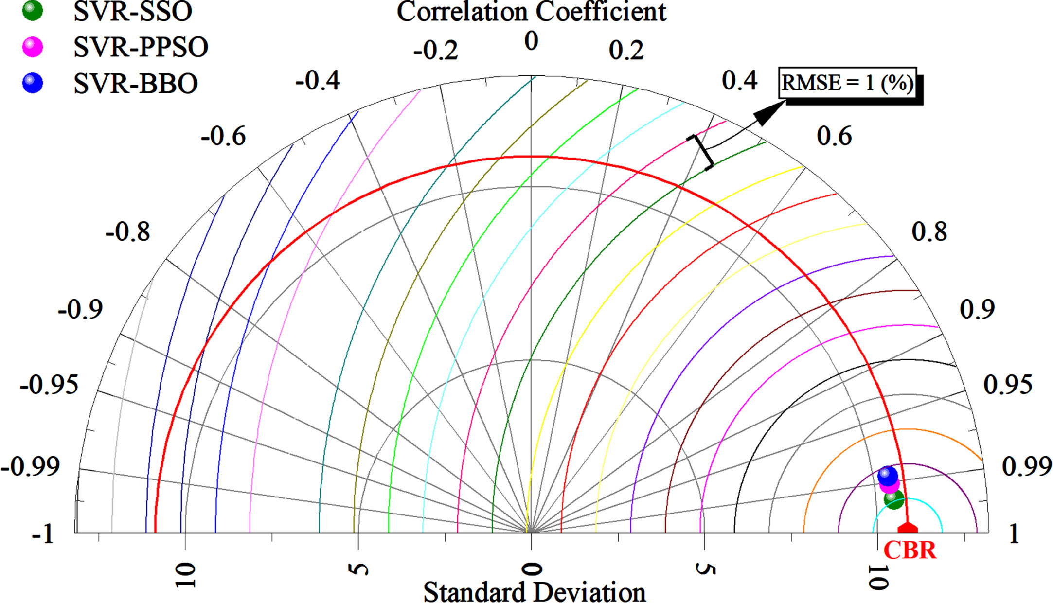
The Taylor diagram for the predicted and measured CBR.
The present study proposed three hybrid models coupled with the support vector regression (SVR) to estimate the California bearing capacity (CBR) of pond ash modified using admixtures. The proposed models include SVR-Biogeography-Based optimization (SVR-BBO), SVR-Particle Swarm Optimization (SVR_PPSO), and SVR-Salp Swarm optimization (SVR-SSO).
It can result that the developed integrated models have R2 bigger than 0.9540. results depict that the agreement between observed and estimated CBR from hybrid algorithms is mainly similar to represent the greatest precision.
The standalone support vector regression (SVR) model exhibited high error rates and a low R2 value, indicating insufficient predictive accuracy. During the training phase, the SVR model achieved an R2 of 0.9615, RMSE of 2.172, MAE of 1.747, and PI of 0.028. A hybridization technique has been obtained to enhance the SVR’s performance. In both the learning and testing stages, SVR-SSO has better performance than the SVR-PPSO and SVR-BBO model, with R2, RMSE, MAE, and PI equal to 0.9894, 1.122, 0.6731, and 0.014 for training data, and 0.9965, 0.819, 0.559, and 0.010 for testing data, respectively. So, by considering the OBJ index, the OBJ value for SVR-SSO is 0.607, lower than SVR-PPSO and SVR-BBO with OBJ values of 1.104 and 1.216, respectively. Therefore, the SVR-SSO model outperforms other models in estimating the CBR of pond ash modified by LI and LS, consequently being recognized as the proposed model.
As it is obvious from the presented figures, in all the proposed hybrid models, the estimated CBR illustrates a remarkable correlation with observed ones, approving developed hybrid models’ potential to estimate the CBR value of pond ash stabilized with LS and LI with great precision. Therefore, both proposed models conclude the lowest error in the CBR forecasting procedure, depicting precise prediction that makes it to be used for practical applications.