A short-term building energy consumption prediction and diagnosis using deep learning algorithms

Abstract

Short-term energy consumption prediction of buildings is crucial for developing model-based predictive control, fault detection, and diagnosis methods. This study takes a university library in Xi’an as the research object. First, a time-by-time energy consumption prediction model is established under the supervised learning approach, which uses a long short-term memory (LSTM) network and a Multi-Input Multi-Output (MIMO) strategy. The experimental results validate the model’s validity, which is close enough to physical reality for engineering purposes. Second, the potential of the people flows factor in energy consumption prediction models is explored. The results show that people flow has great potential in predicting building energy consumption and can effectively improve the prediction model performance. Third, a diagnostic method, which can recognize abnormal energy consumption data is used to diagnose the unreasonable use of the building during each hour of operation. The method is based on differences between actual and predicted energy consumption data derived from a short-term energy consumption prediction model. Based on actual building operation data, this work is enlightening and can serve as a reference for building energy efficiency management and operation.

Keywords

Deep learning energy consumption prediction energy consumption diagnosis people flows

1 Introduction

As China’s economy grows, it has become a market that has a huge impact on the structure of world energy supply and demand [1]. In the medium-to-long-term outlook for global energy supply and demand, China’s economy will continue to rise significantly, as will its energy need. Excessive energy consumption not only leads to the depletion of fossil fuels like oil and coal, which seriously threatens the sustainability of natural resource use but also leads to massive greenhouse gas emissions and hasten the process of global warming [2]. Therefore, promoting efforts to ensure stable energy supply and demand and to address energy and environmental issues will be key to world energy security.

Currently, the building sector accounts for 39 percent of total global energy consumption and 38 percent of total global greenhouse gas emissions, respectively [3]. Compared to the transportation and industrial sectors, buildings have much greater energy-saving potential [4]. At the same time, with the gradual rise in floor space and energy consumption in recent years [5], energy efficiency research has become an important research direction, and fast and accurate energy consumption forecasting can provide data to optimize operational efficiency and help achieve China’s peak CO₂ emissions by 2030.

In the process of building utilization, energy consumption is influenced by occupant behavior and external conditions such as climate and is regular and cyclical [6]. To reduce the waste of energy consumption in buildings, there is an urgent need to establish scientific predictive and diagnostic models based on in-depth analysis of the influencing factors and to take practical measures.

The goal of this research is first to develop a short-term prediction model for building energy consumption based on deep learning algorithms and to investigate the effect of the people flows factor on prediction performance. Then, based on the prediction model, an abnormal energy consumption diagnosis model is established to compare the predicted energy consumption values with the measured energy consumption values to determine the abnormal energy consumption and diagnose the unreasonable usage phenomena in building operations. Finally, the diagnostic results are applied to building operations and energy efficiency management.

The remainder of this paper is structured as follows: Section 2 reviews the literature relevant to this study. Section 3 presents the theoretical foundations of the algorithms and strategies used in this paper. Section 4 provides a detailed study of the case. A discussion of the case results is presented in Section 5. Section 6 summarizes the conclusions.

2 Literature review

For a long time, the industry has undertaken a comprehensive and in-depth study on building energy consumption prediction and achieved remarkable results. The existing methods are classified into two main categories: physical methods and data-driven methods. The prediction accuracy of physical methods relies heavily on detailed information about the building system [7] and the model performance may be inconsistent if the assumptions of physical principles are not satisfied [8]. In contrast, data-driven methods, which obtain historical building energy consumption sample data through sensing and communication technologies [9] and establish nonlinear mapping relationships between energy consumption samples, have been widely used in building energy consumption prediction due to their practicality, adaptability, and high prediction accuracy [10]. Previous studies have shown that prediction techniques in machine learning and artificial intelligence, such as artificial neural networks (ANN) [11] and support vector regression (SVR) [12, 13], work well in building energy consumption prediction. Data-driven approaches are gaining popularity in the building sector as modern building automation systems (BAS) provide more and more data on building operations. The rapid development of big data analytics opens up possibilities for making effective use of BAS data. A prominent and promising example is deep learning, which has achieved great success in the field of pattern recognition [14]. Deep learning can be developed both in a supervised manner for deep neural networks (DNN) models for prediction and in an unsupervised manner for deep autoencoder models for feature extraction [15]. Lee et al. [16] used a deep learning approach to integrate the advantages of supervised and unsupervised learning to build prediction models and improve the prediction efficiency of heating ventilation and air conditioning (HVAC) systems.

In general, time series and regression are the most often utilized data-driven methods for building energy consumption prediction. The former predict building energy consumption over time by identifying interdependencies and correlations between variables and time; the latter predict building energy consumption through building models based on the correlation between numerous attributes and energy consumption data [17]. Traditional machine learning techniques treat each input variable as an independent variable and therefore ignore the inherent temporal dependence between successive measures. Recurrent neural networks (RNN) use a continuous approach to input data, and therefore, the temporal dependence between continuous data can be well captured [18]. It has been shown that recurrent models achieve superior accuracy in energy prediction relative to other popular machine learning techniques [19, 20].

The role of energy consumption forecasting varies depending on the forecasting period. Long-term forecasts (e.g., more than one year) are typically used for energy maintenance planning [21]and power distribution [22]; medium-term forecasts (e.g., monthly, annually) are mainly used for component operation mode determination [23] and predictive maintenance [24]; and short-term forecasts (e.g., sub-hourly, hourly, or daily) are typically used for predictive model control [25], fault detection [26], and control optimization [27]. Short-term building energy consumption forecasting has attracted a great deal of interest among building professionals because of its close relevance to the daily operation of various service systems [28, 29]. Accurate prediction of building electricity consumption enables smooth integration of individual buildings with smart grid infrastructure [30], identifies abnormal operating behavior [31, 32], and optimizes the operation strategy of building renewable systems [33]. Shan et al. [34] developed a robust chiller sequence control strategy based on predicted building cooling load. The strategy was validated to be 3% more energy efficient than the conventional strategy. The predicted cold load was used directly or indirectly as an indicator for fault detection and diagnosis (FDD). Ben et al. [35] used ANN to predict the next day’s cold load and optimize the HVAC thermal storage system operation. The results showed that the optimal control strategy can reduce operating costs while improving operational flexibility. Wang et al. [36] proposed a method for predicting power consumption and detecting anomalies based on long short-term memory (LSTM) neural network, which resulted in a significant improvement in power theft identification compared with previous unsupervised algorithms. One of the studies’ underlying assumptions is that reliable short-term building load forecasting is available.

A data-driven dynamic energy diagnostic approach based on data has received increasing attention because it can provide accurate results by comparing current energy performance with historical data. The key to using a data-driven approach for energy consumption anomaly diagnosis is to build a reasonable and effective energy consumption prediction model that compares predicted values with historical energy consumption values to diagnose a building’s energy use and help operators identify abnormal energy use and inefficient operating conditions. Examples include Energy Star in the US [37], Demonstrated Energy Certificate (DEC) in the UK [38], and Leadership in Energy and Environmental Design (LEED) in Chicago [39]. Park et al. [40] use three data mining techniques (correlation analysis, decision tree analysis, and variance analysis) to propose an energy benchmark for improving the operational rating system of 1072 office buildings in Korea. Lin et al. [41] propose a temperature-based approach with simulation tests to detect abnormal energy failures in building operations. Yan et al. [42] propose a multi-level energy performance diagnosis method for buildings where energy information is scarce and energy use data is very limited. Li et al. [43] proposed a simplified method for energy benchmarking of HVAC systems in large commercial buildings based on detailed data from sub-metering systems and overall building operation. Liu et al. [44] proposed a support vector machine method for predicting and diagnosing energy consumption in large public buildings based on 11 input parameters such as historical energy consumption data, meteorological data, and time-period data. Traditional building energy diagnostic methods are based on benchmarks identified in national or local codes and compare the energy performance of reference buildings by building thermodynamic models. However, the results of such diagnostic methods are often difficult to interpret, while failing to provide targeted observations.

The application of building energy prediction in energy diagnosis was discussed previously, and the following information was obtained from a literature review.

The use of deep learning algorithms for building energy consumption prediction and diagnosis has been less studied in applications.

Previous studies on building energy consumption prediction only took the number of people inside the building as an input parameter and did not consider the impact of entrance and exit personnel flow on the building energy prediction model.

Existing building abnormal energy consumption diagnosis usually uses a daily or monthly benchmark, which is challenging at smaller time scales.

To address the current research gaps, the main objectives of this study are as follows.

A multi-step ahead short-term building energy consumption prediction model is developed based on 10 input parameters including historical energy consumption data, people flow, meteorological factors, and temporal factors. This model is performed under a supervised learning approach using LSTM networks and the Multi-Input Multi-Output (MIMO) strategy.

Classify people flows into three categories according to the movement of people and analyze the impact on the performance of the building energy consumption prediction model.

The abnormal energy consumption diagnosis method is developed on a smaller time scale (per hour) based on a short-term energy consumption prediction model. Then, based on the diagnosis results, an in-depth analysis of abnormal energy consumption is conducted.

3 Theoretical background

3.1 Long short-term memory

For sequential problems, recurrent neural networks can be used, which have been successfully applied to many problems such as neuro-linguistic programming, speech recognition, and machine translation [18]. In theory, RNN can make use of information in arbitrarily long sequences. However, in practice, the deepening of the network structure makes the model lose the ability to learn prior information and is limited to looking back only a few steps. A typical RNN is depicted in Fig. 1.

Fig. 1

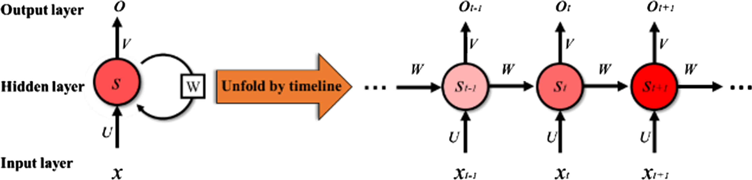
RNN network structure.

One of the most popular solutions is called the long short-term memory neural network. LSTM was first proposed by Hochreiter & Schmidhuber in 1997 [45], which can effectively solve the problem of long-term dependence of information and avoid gradient disappearance or explosion. Broadly speaking, LSTM is a special model in RNN, which also has the recursive property of RNN. Narrowly speaking, it is again a modified model of RNN with a distinct memory and forgetting pattern that can be flexibly adapted to the timing characteristics of network learning tasks. Compared to the traditional RNN, the hidden layer of LSTM is no longer an ordinary neural unit, but rather an LSTM unit with a distinct memory pattern. The cell of the LSTM model is depicted in Fig. 2. The LSTM model uses the sigmoid function and the tanh function to process the data. They are expressed as:

Fig. 2

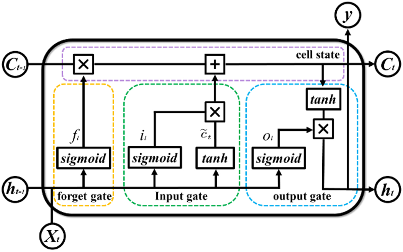
LSTM structure.

$sigmoid (z) = \frac{1}{1 + e^{- z}}$ (1) $tanh (z) = \frac{e^{z} - e^{- z}}{e^{z} + e^{- z}}$ (2) where e ≈ 2.7183, sigmoid (z) ∈ [0, 1], and tanh(z) ∈ [- 1, 1].

The function of the forget gate is to decide which relevant information from the previous step should be discarded or retained. The information from the previous hidden layer and the current input are passed to the sigmoid function at the same time, and the output value ranges between 0 and 1. The closer it is to 0, the more it should be discarded, and the closer it is to 1, the more it should be kept. $f_{t} = sigmoid (W_{f} \cdot [h_{t - 1}, x_{t}] + b_{f})$ (3)

The function of the input gate is to determine which information is important in the current input. Firstly, the previous hidden layer’s information and the current input are passed to the sigmoid function, and the value is adjusted to a value between 0 and 1 to determine which information to update. Next, the previous hidden layer’s information and the current input are passed to the tanh function to generate a new marquee vector. Finally, the output value of the sigmoid function is multiplied by the output value of the tanh function. $i_{t} = sigmoid (W_{i} \cdot [h_{t - 1}, x_{t}] + b_{i})$ (4) ${\tilde{c}}_{t} = tanh (W_{c} \cdot [h_{t - 1}, x_{t}] + b_{c})$ (5)

The cell state runs through the entire process. Firstly, the cell states of the previous layer are multiplied point by point with the oblivion vector. Finally, the value is added point by point with the output value of the input gate to update the neural network’s new information into the cell state. $C_{t} = f_{t} \times C_{t - 1} + i_{t} \times {\tilde{c}}_{t}$ (6)

The output gate’s function is to determine the value of the next hidden layer. Firstly, the previously hidden layer and the current input information are passed to the sigmoid function, and the newly obtained cell state is passed to the tanh function. Finally, the sigmoid function output is multiplied by the tanh function to determine the information that the hidden state should carry and pass to the next time step. $o_{t} = sigmoid (W_{o} \cdot [h_{t - 1}, x_{t}] + b_{o})$ (7) $h_{t} = o_{t} \times tanh (C_{t})$ (8)

Where W_f, W_i, W_c, W_o and b_f, b_i, b_c, b_o are the corresponding weights and biases, respectively.

3.2 Multi-step ahead time series forecasts

A Multi-step ahead time series forecasting implies applying historical time series [y₁, y₂, . . . , y_N] to predict the subsequent H-step series [y_N+1, y_N+2, . . . , y_N+H], where N denotes the number of observed data and H≥1 denotes the prediction range [46, 47]. It can be generated by iterating a single-step ahead model or directly using a specific model for each period. It has been widely used for short-term building energy forecasting due to the strong time dependence of building energy consumption between each time step [48].

Good forecasting is an important basis for people to make decisions. This paper examines the performance of three primary strategies for multi-step ahead time series forecasting: the Recursive strategy, the Direct strategy, and the Multi-Input Multi-Output (MIMO) strategy. The recursive strategy is the most traditional and intuitive multi-step ahead prediction strategy [49]. For historical time series [y₁, y₂, . . . , y_N], The prediction model can be expressed as: $y_{t + 1} = f (y_{t}, y_{t - 1}, . . ., y_{t - d + 1}) + w$ (9) where t∈ { d, . . . , N - 1 }, w is the noise vector, d is the embedding dimension, and f denotes the correlation function between past observations.

When we forecast H steps ahead, the first step is predicted by the model, then the next step (use the same one-step-ahead prediction mode) is predicted using the value just predicted as part of the input variable, and so on until the full horizon is forecasted. The prediction process is as follows: ${\hat{y}}_{N + h} = {\begin{matrix} \hat{f} (y_{N}, . . ., y_{N - d + 1}) & if & h = 1 \\ \hat{f} ({\hat{y}}_{N + h - 1}, . . ., {\hat{y}}_{N + 1}, y_{N}, . . ., y_{N + h - d}) & if & h \in {2, . . ., d} \\ \hat{f} ({\hat{y}}_{N + h - 1}, . . ., y_{N + h - d}) & if & h \in {d + 1, . . ., H} \end{matrix}$ (10)

Since the recursive strategy relies on a one-step prediction model throughout the training cycle, there is a high possibility of error accumulation when the prediction time horizon is long and all model inputs are predicted values. For the error accumulation problem of the recursive strategy, the direct strategy develops a separate model (Eq. (11)) for each time step in the prediction time horizon and does not use any predicted values for the next prediction step, so it is not affected by the error accumulation. $y_{t + h} = f_{h} (y_{t}, y_{t - 1}, . . ., y_{t - d + 1}) + w$ (11) with t∈ { d, . . . , N - H } , h ∈ { 1, . . . , H }.

The entire prediction process of the direct strategy can be defined as: ${\hat{y}}_{N + h} = {\hat{f}}_{h} (y_{N}, . . ., y_{N - d + 1})$ (12)

Since multiple models are developed, a large computational load is generated. In addition, since the prediction models are generated independently of each other, the complex temporal correlation between the predictions is ignored, thus affecting the overall prediction accuracy. Considering the complex dependencies between variables, one possible solution is to move from modeling single-output mappings to modeling multiple outputs.

MIMO strategy, as the name implies, is a process of multiple target output. As shown in Fig. 3, it avoids the Direct strategy’s conditional independence assumption as well as the Recursive strategy’s error accumulation. The prediction model can be expressed as: $[y_{t + H}, . . ., y_{t + 1}] = F [y_{t}, y_{t - 1}, . . ., y_{t - d + 1}] + w$ (13) where F denotes the correlation function between future predicted values.

The prediction process can be defined as: $[{\hat{y}}_{t + H}, . . ., {\hat{y}}_{t + 1}] = \hat{F} [y_{N}, y_{N - 1}, . . ., y_{N - d + 1}]$ (14)

Fig. 3

The inference mechanism of MIMO strategy.

3.3 Prediction performance evaluation metrics

To evaluate the prediction model’s accuracy, residuals (ɛ) are used to reflect the prediction accuracy of each time step, while mean absolute error (MAE) shows the overall accuracy. ɛ and MAE can be expressed as below: $ɛ = y_{i} - {\hat{y}}_{i}$ (15) $MAE = \frac{\sum_{i = 1}^{n} | y_{i} - {\hat{y}}_{i} |}{n}$ (16) where n is the sample size, i is the prediction point sequence number, y_i is the actual energy consumption value, and ${\hat{y}}_{i}$ is the predicted energy consumption value.

Similarly, root mean squared error (RMSE) and MAE are scale-dependent metrics that describe the error between the predicted value and the actual value. The RMSE is most sensitive to anomalous data because it geometrically amplifies the error and can be expressed using: $RMSE = \sqrt{\frac{\sum_{i = 1}^{n} {(y_{i} - {\hat{y}}_{i})}^{2}}{n}}$ (17)

The coefficient of variation of the root mean squared error (CV-RMSE) is a scale-independent index that indicates the relative size of the error. $CV - RMSE = \sqrt{\frac{\sum_{i = 1}^{n} {(y_{i} - {\hat{y}}_{i})}^{2}}{n}} / - \frac{\sum_{i = 1}^{n} y_{i}}{n}$ (18)

The coefficient of determination (R²) measures the degree of fit of the prediction model. A larger R² indicates a better prediction performance. The R² is defined by the formula: $R^{2} = 1 - \frac{\sum_{i = 1}^{n} {(y_{i} - {\hat{y}}_{i})}^{2}}{\sum_{i = 1}^{n} {(y_{i} - {\bar{y}}_{i})}^{2}}$ (19) where R² ∈ [0, 1], and ${\bar{y}}_{i}$ is the average of the actual energy consumption.

4 Case study

4.1 Research outline

The structure of a short-term building energy consumption prediction and diagnosis using deep learning algorithms is shown in Fig. 4. It consists of two phases: prediction and diagnosis. The goal of the first phase is to develop a supervised short-term energy consumption prediction model that uses an LSTM network optimized for MIMO strategies. The model is applied to a real building to evaluate the prediction performance and to investigate the effect of people flow factors on the performance of the energy prediction model. In the second phase, based on the short-term energy consumption prediction model, the predicted values of each step are compared with the actual values to determine the abnormal energy consumption diagnosis criteria. The established abnormal energy consumption diagnostic criteria are applied to actual buildings to detect unreasonable use and improve energy use efficiency.

Fig. 4

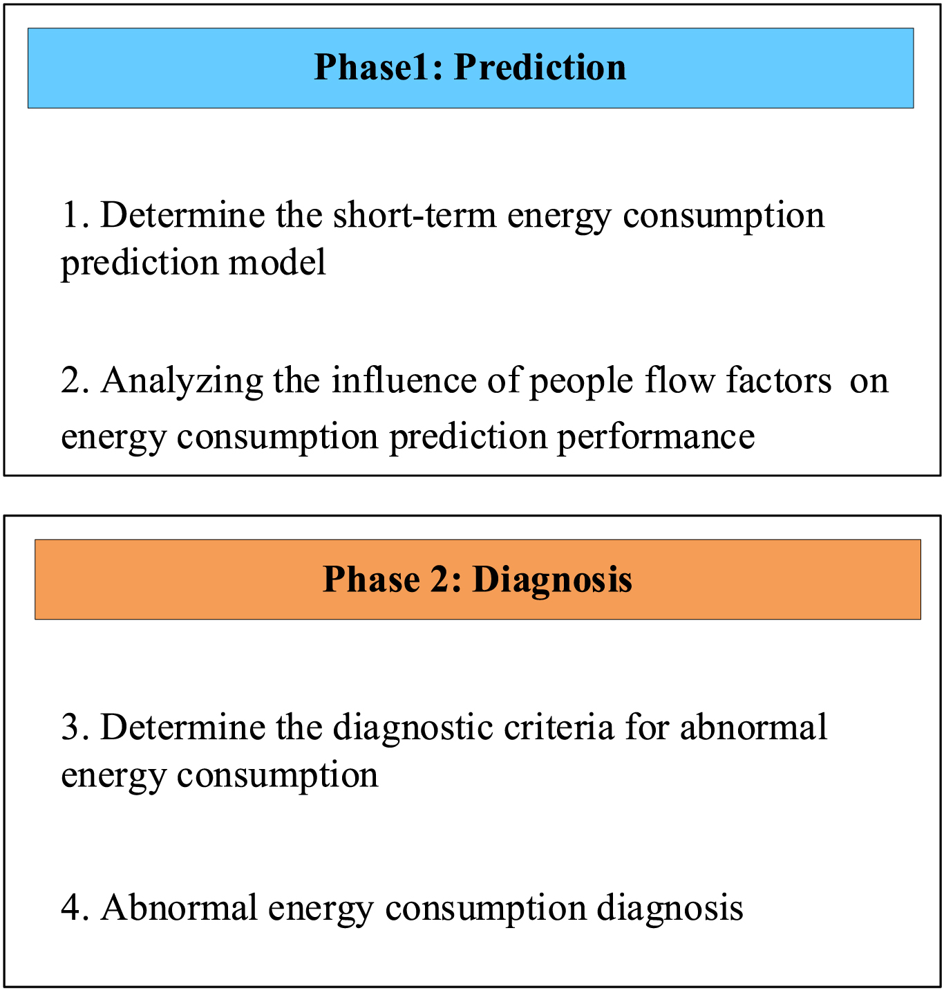
Research outline.

4.2 Data description

In this paper, we selected the Yanta Campus Library of Xi’an University of Architecture and Technology, China, as the simulated building. As shown in Fig. 5, the library is a five-story building which has a floor area of 12,700m² and 1,200 reading seats. It is mainly divided into book stacks, reading rooms, lecture halls, study areas, office areas, etc.

Fig. 5

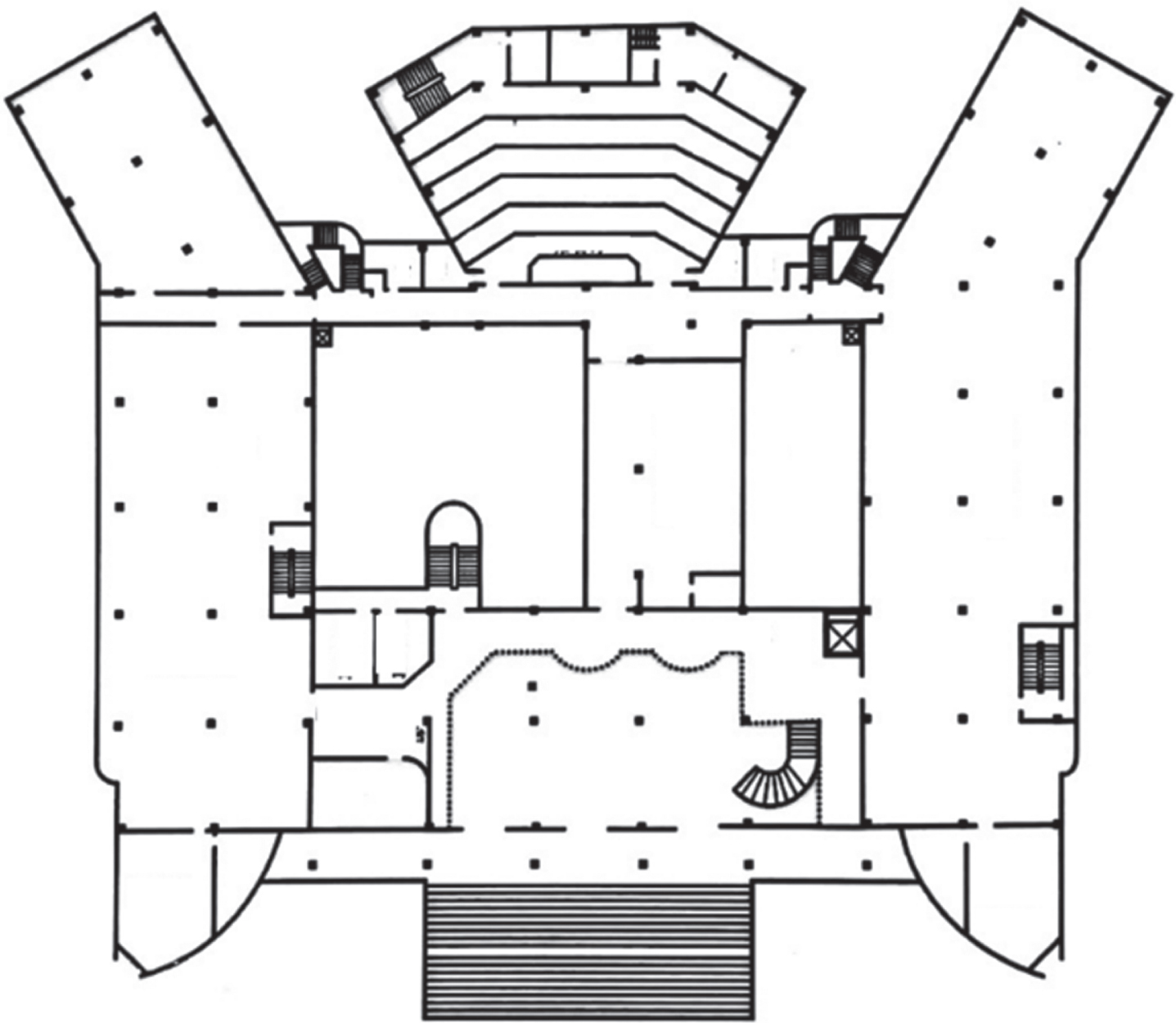
Library floor plan.

The input variables include historical energy consumption data, people flow, meteorological factors (e.g., outdoor temperature, relative humidity), and temporal factors (e.g., time of day, workday type), as shown in Table 1. The energy consumption data came from the school’s energy monitoring platform, which captures energy use in all school buildings. The authors downloaded the library energy use from this system on average every hour. It is important to emphasize that electricity is considered the only source of energy for the library, except for the use of municipal heating from November 15 to March 15 of each year. People flow data came from the library’s Access Control Information Query Statistics System (ACIQSS). All people entering and leaving the library must pass through face recognition and are allowed to pass one person at a time. Based on the information provided by ACIQSS, it was converted into the data type required for the experiment. Meteorological data were obtained from local weather stations. In addition, the workday type was presented, which was derived from the academic calendar of the University.

Table 1

Summary of input variables

Variable	Abbreviations	Measurement
Historical energy consumption	HEC	kW·h
Visitors flow into the library	Into	Individual
Visitors flow out of the library	Out	Individual
In-library flow	In	Individual
Outdoor temperature	Ot	°C
Relative humidity	Rh	%
Solar radiation	Sr	kW·h/m²
Wind speed	Ws	m/s
Time of day	T	1, 2, 3, . . . , 22, 23, 24
Workday type	W	Weekday and weekend
Day type	D	Sunday, Monday, . . . , Saturday

The output variables are the electricity consumption of the library, covering electricity for lighting sockets, electricity for air conditioning, electricity for power, etc. Figure 6 depicts in detail the hourly electricity consumption of the library from September 2020 to October 2021.

Fig. 6

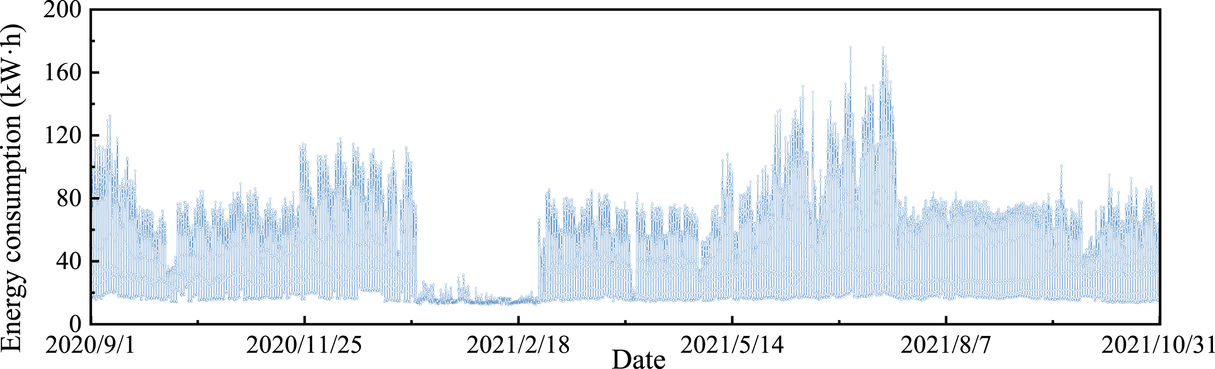
Power consumption per hour.

4.3 Data pre-processing

Before the model is trained and tested, the raw data is initially analyzed and pre-processed to understand the relationship between input and output variables, and the most important variables are selected to reduce the complexity of model training and improve prediction accuracy. Of course, using multiple inputs is well connected to the predicted reality, however, introducing too many variables can make the model more complex and introduce uncertainty into the system by over-relying on known variables. Objectively, this connection is made to justify the use of fewer input parameters to achieve satisfactory prediction performance and accuracy.

Figure 7 shows the results of the Pearson correlation analysis between the different features and energy consumption in the collected raw data set. The results show that: outdoor temperature, visitors flow into the library, and in-library flow have a strong correlation with the energy consumption of the library; in-library flow has the strongest correlation with the energy consumption, and the wind speed has the lowest correlation with the energy consumption.

Fig. 7

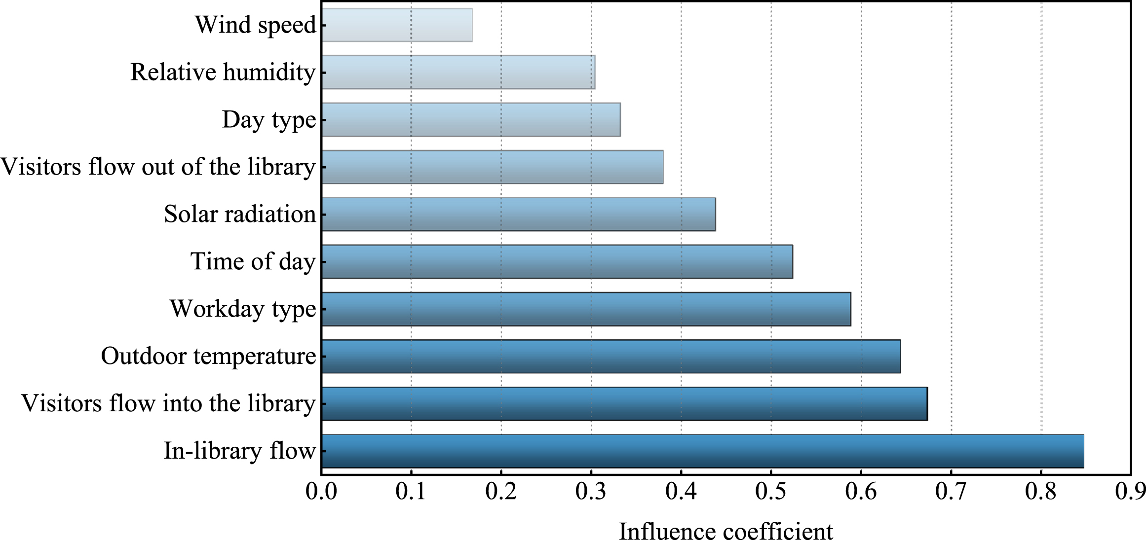
Variable correlation.

According to the Pearson correlation significance criteria, the features with correlation coefficients greater than 0.3 were selected as the input parameters of the prediction model. Therefore, 10 parameters such as historical building energy consumption, in-library flow, visitors flow into the library, and outdoor temperature with correlation coefficients greater than 0.3 were used as inputs to the building energy consumption prediction model for model learning and testing.

For the problem of missing data, the average value of this data for 2 similar days in the vicinity is taken to fill in. If the data suddenly becomes abnormally large or suddenly becomes 0, the data is replaced by the data of the time period before and after the time of this data and the data of similar days. Quantifies the type of weekday (e.g., weekdays are set to 1 and weekends are set to –1).

When multivariate time series are used for energy consumption forecasting, the magnitudes differ between variables and the values vary widely. Considering the range of inputs and outputs of the nonlinear activation function in the model, to avoid saturation of neurons and to consider equally the role of each variable on building energy consumption, Eq. (20) was used to normalize the raw data to the interval [–1, 1]. $x^{'} = \frac{x - (x_{max} + x_{min}) / - 2}{(x_{max} - x_{min}) / - 2}$ (20) where x′represents the normalized data, x represents the data before normalization, x_max and x_min are the extreme and minimal values of the variable, respectively.

The predicted building energy consumption data obtained by the prediction model is then inverse normalized to make it physically meaningful, and the inverse normalization is calculated by the formula: $x = \frac{1}{2} [x^{'} (x_{max} - x_{min}) + (x_{max} + x_{min})]$ (21)

4.4 Predictive model design

The energy consumption prediction model was implemented on an Intel(R) Core (TM) i7-10870 H CPU @ 2.20 GHz system, using PyCharm professional edition 2021.2 and the Anaconda3 development environment, built on the TensorFlow framework and Python 3.7.

Traditional prediction models split the data set into two parts: the training set (about 70%) and the test set (about 30%). To be able to select the model with the best effect and generalization ability. In this study, the entire dataset is divided into training set (about 60%), validation set (about 20%), and test set (about 20%). The training set is used for model training; the validation set is used to determine the model hyperparameters and select the optimal model, and the test set is used for prediction result verification and anomaly diagnosis.

In this paper, we use the LSTM algorithm and MIMO strategy with a supervised learning method for short-term energy consumption prediction, and the design process is shown in Fig. 8. Seven types of hyperparameters were optimized by grid search, including Hidden size, Epochs, Dropout, Batch size, Optimization method, Activation function, and Loss function. Grid search settings are shown in Table 2. Among them, Input size and Output size are determined by the model structure.

Fig. 8

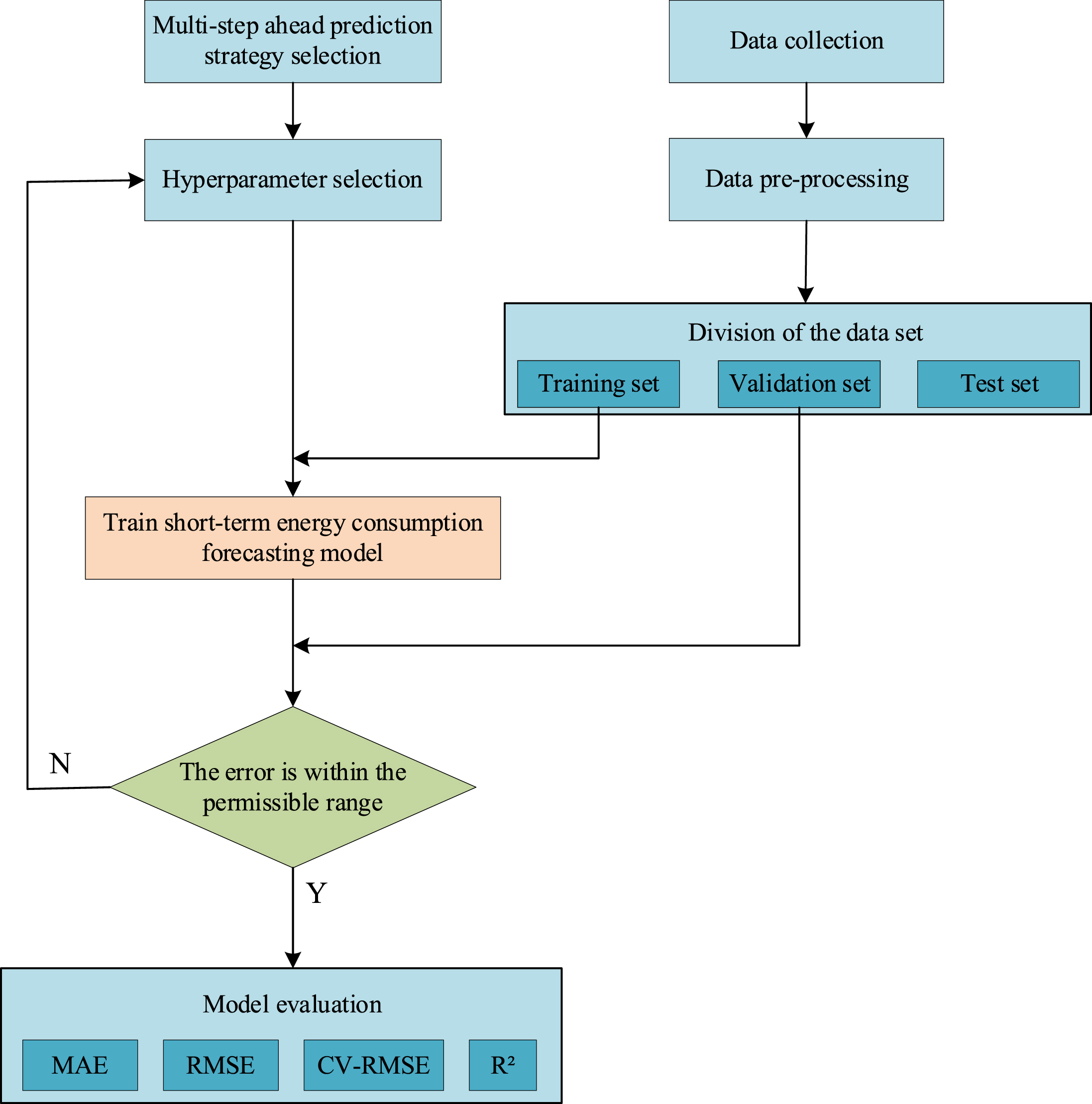
Flow chart of energy consumption prediction.

Table 2

Hyperparameter settings

Hyperparameter	Grid-search values	Values
Input size	10	10
Hidden size	1, 2, 3, 4, 5	3
Output size	1	1
Epochs	50, 100, 150, 200	100
Dropout	0, 0.01, 0.05, 0.1, 0.15, 0.2	0.01
Batch size	12, 24, 32, 64	24
Optimization method	Adam, SGD, RMSprop, Momentum	Adam
Activation function	Sigmoid, Relu, tanh	Relu
Loss function	Mean square error, Cross Entropy	Mean square error

4.5 Diagnostic criteria for abnormal energy consumption

The criteria for judging energy consumption anomalies are mainly based on the error value between energy-saving data and non-energy-saving data (the data obtained from the prediction model is energy-saving data and the actual data is non-energy-saving data), while the ideal situation is that the two are the same, or the actual energy consumption is less than the predicted energy consumption, indicating that the current energy consumption is reasonable and in an energy-saving state. Usually, the gap between actual energy consumption and predicted energy consumption is inevitable due to the perturbation of various uncertainties.

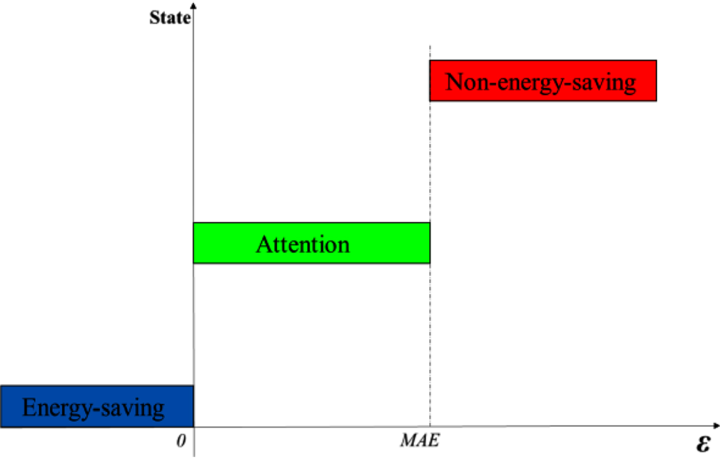
A simple and practical diagnosis method for abnormal energy consumption in buildings is essential for building energy efficiency. Traditional diagnosis methods have complicated processes, so this paper proposes an abnormal energy consumption diagnosis method based on a prediction model, which uses the deviation between the predicted energy consumption and the actual value and has the advantages of fast diagnosis, high diagnostic accuracy, and practicality. The established short-term energy prediction model is used as a benchmark for energy consumption anomaly diagnosis to evaluate the energy consumption at each time step, and the design process is shown in Fig. 9. ɛ is used to indicate the difference between the actual energy consumption and the predicted value in the diagnostic data. MAE indicates the mean absolute error of the predicted data with the actual value greater than the predicted value. As is shown in Fig. 10, when ɛ is less than or equal to 0, it is considered an energy-saving state at this time; when ɛ is greater than 0 and less than or equal to MAE, it is considered an attention state at this time, and there may be a non-energy-saving situation; when ɛ is greater than MAE, it is considered as a non-energy-saving state at this time, and there is the non-energy-saving situation, which needs to be analyzed and managed to eliminate abnormalities.

Fig. 9

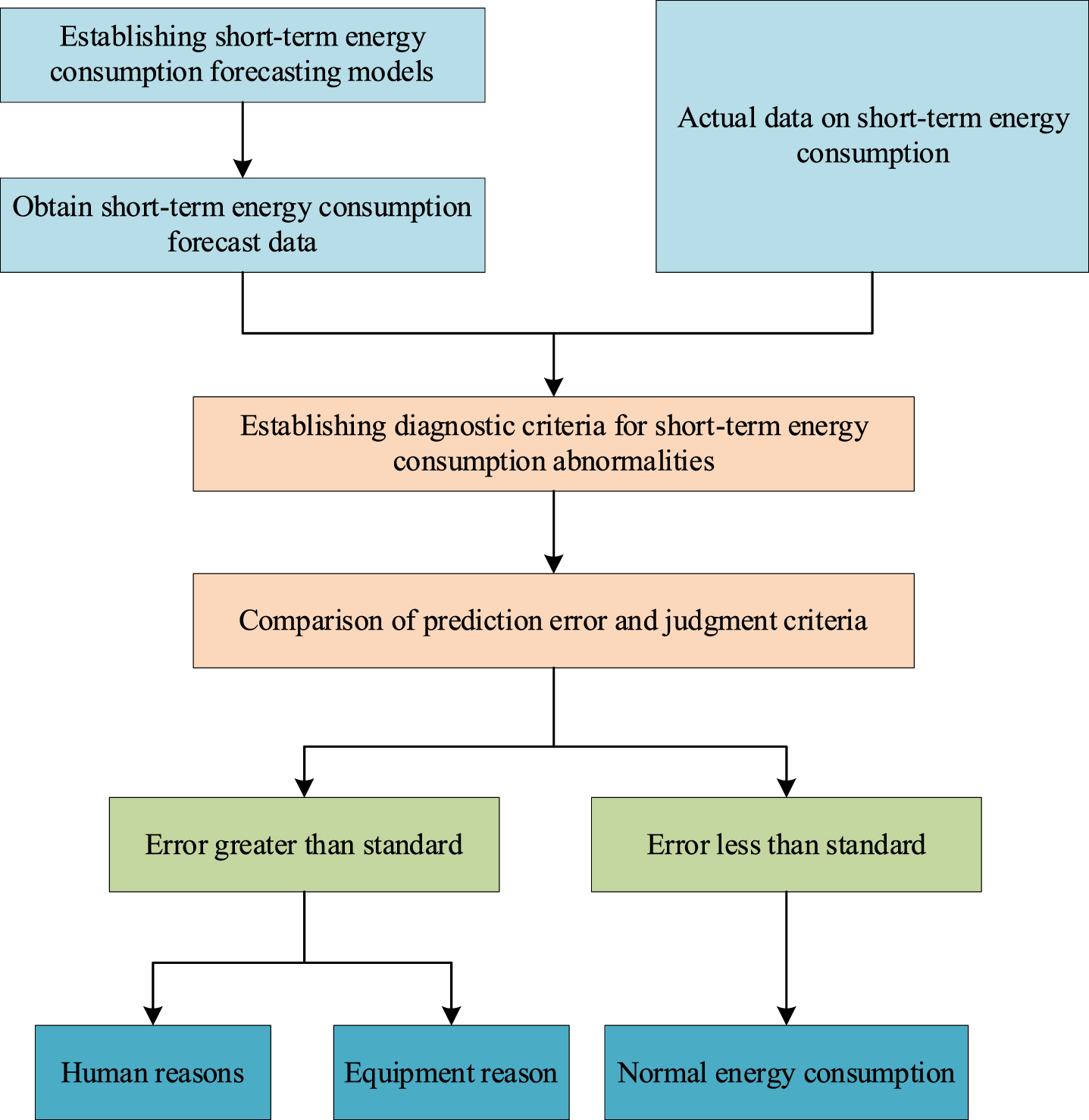
Flow chart of abnormal energy consumption diagnosis.

Fig. 10

Energy consumption state determination standard.

Algorithm 1: Diagnostic Analysis
Input:
Historical energy consumption data (H_i), People flow data
(P_i), Meteorological factor data (M_i), Temporal factor data (T_i)
Operation process:
Train the MIMO-LSTM model
Choose the right hyperparameters
Calculate ɛ using the Equation (15)
Calculate MAE using the Equation (16)
For each attribute i in the diagnostic dataset
if ɛ≤0; DR is the set Energy-saving
if 0<ɛ≤MAE; DR is the set Attention
if ɛ>MAE; DR is the set Non-energy-saving
End for
Output:
Diagnostic result (DR)

5 Results and discussion

5.1 Short-term energy prediction results

In this study, data related to energy consumption from September 2020 to April 2021 were selected to train the model, data from May to July 2021 were used as the validation data, data from August and September were used as the prediction data, and finally, data from October were selected to diagnose abnormal energy consumption.

Figure 11 shows the building energy consumption predicted 24 hours in advance versus the actual energy consumption for the period from August to September 2021, and the model had a good predictive performance overall, except for the peak prediction. To verify the effectiveness of the model proposed in this paper, it is compared with traditional machine learning methods, as shown in Table 3, and the MIMO-LSTM model outperforms other models in all performance indexes. According to the literature, if the CV-RMSE is less than 30% when using hourly data, the model is sufficiently close to the physical reality for engineering purposes [50]. As listed in Table 3, the CV-RMSE of the model proposed in this paper is 0.1434, which was far below the 30% threshold, indicating that the predictive performance of the model was reliable for subsequent energy consumption anomaly diagnosis.

Fig. 11

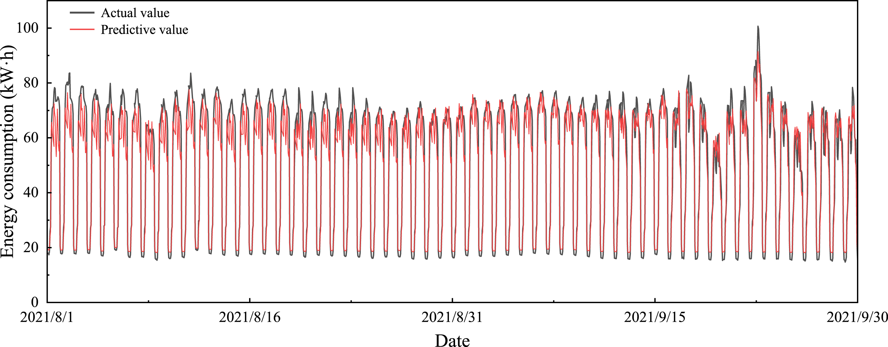
Predicted results of the prediction set.

Table 3

Summary of prediction results of different models

	MAE	RMSE	CV-RMSE	R²
DT	12.1029	17.6273	0.3112	0.5871
SVR	11.8327	15.5890	0.2618	0.6187
BP	10.5319	13.4092	0.2291	0.7366
RBF	8.1483	10.0873	0.1829	0.8029
LSTM	6.0163	8.1521	0.1586	0.8863
MIMO-LSTM	5.5582	7.4744	0.1434	0.9001

5.2 Influence of people flow

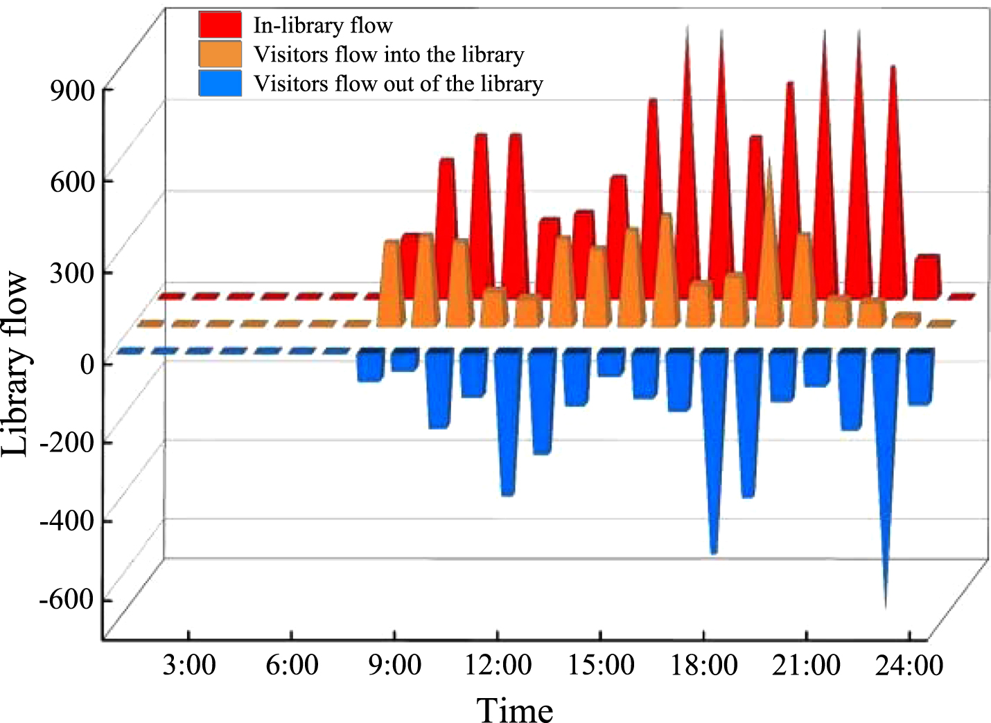
To further explore the effect of people flow factors on the predicted performance of library energy consumption, people flow factors were divided into three categories: in-library flow, visitors flow out of the library, and visitors flow into the library. As shown in Fig. 12, during the library opening hours (7 a.m. to 11 p.m.), the number of people in the library shows three peaks, which occur at 10 a.m., 4 p.m. and 8 p.m.; differently, the number of people leaving the library peaks at 12 a.m., 6 p.m. and 11 p.m., respectively.

Fig. 12

Fluctuating library population change.

Figure 13 shows the actual energy consumption on September 15, 2021, versus the projected energy consumption with different input characteristics. Unlike the change in the number of people, there were two peaks in actual energy consumption, at 11:00 a.m. and 4:00 p.m. There was no significant increase in energy consumption at 8:00 p.m. when the number of people peaked for the third time. The main reason for this is that the nights are cooler in autumn and the demand for air conditioning does not increase significantly when the number of people increases, and there was a difference in time between the peak number of people and the peak energy consumption due to the lagging nature of the air conditioning system. As can be seen from Fig. 13, the best prediction performance was achieved when all three features (visitors flow into the library, visitors flow out of the library, and In-library flow) are input, while the worst prediction performance was achieved when only visitors flow out of the library was available.

Fig. 13

Forecast results for different input features.

As shown in Table 4, the evaluation metrics of the model prediction under different input features are shown in detail. Compared with single input features, the prediction performance of the model with multiple input features is significantly improved. For a single feature, the in-library flow has the greatest impact on the improvement of prediction performance, followed by the visitors flow into the library, and the least impact is the visitors flow out of the library. Table 4 also shows that people flow had great potential for predicting building energy consumption. With all three features input, the prediction model is optimal for all indicators.

Table 4

Prediction accuracy with different input features

	MAE	RMSE	CV-RMSE	R²
Out	13.9673	18.6436	0.3577	0.3785
Into	12.6653	15.9528	0.3061	0.5450
In	11.1165	14.9488	0.2868	0.6005
Into + Out	9.7128	12.3402	0.2368	0.7277
Out + In	8.2788	11.2612	0.2161	0.7733
Into + In	6.9919	8.9554	0.1718	0.8566
Into + Out + In	5.5582	7.4744	0.1434	0.9001

People flow is a major source of uncertainty in building energy prediction models. In this study, relatively static data on changes in the number of people over one hour are used; whereas occupant behavior is dynamic, stochastic, and influenced by various factors. Nonetheless, the expected results are still achieved in this study.

5.3 Abnormal diagnosis of energy consumption

The established model was applied to the energy consumption forecast for October. Based on forecast results, the deviation of the predicted energy consumption from the actual energy consumption was calculated for each step. Figure 10 shows the proposed energy consumption judgment criteria, which were divided into three cases: energy-saving state, attention state, and non-energy-saving state. As shown in Fig. 14, when the deviation between the actual value and the predicted value is less than or equal to 0, the state of energy-saving is considered; when the deviation is greater than 0 and less than or equal to 7.8253 (the average absolute error of the test set in the non-energy saving state), the state of attention is considered; when the deviation is greater than 7.8253, the state of non-energy saving is considered.

Fig. 14

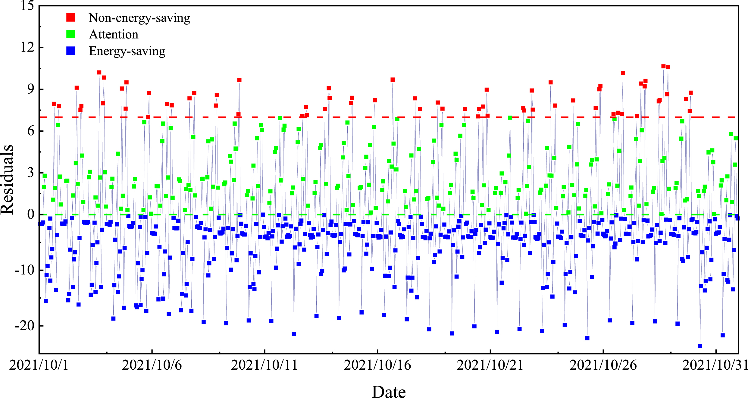
Energy consumption diagnosis results.

Table 5 provides statistics on the distribution of diagnostic results among the three states. Among the 744 data in October, 67 data were diagnosed as non-energy-saving status, accounting for 9.01% of the total data in October; 220 data were diagnosed as attention status, accounting for 29.57% of the total data; and 457 data were diagnosed as energy-saving status, accounting for 61.42% of the total data. Table A1 shows in detail the results of energy consumption in a non-energy saving state in October. Among the 67 non-energy-saving states, they are mainly concentrated at 5 p.m., 9 p.m., and 10 p.m. and a small number of them occurred at 11 a.m. and 12 a.m. Three of these time points had a relative error of 20% or more.

Table 5

Statistics of diagnosis results of three states

State	Number	Percentage of total
Non-energy-saving	67	9.01%
Attention	220	29.57%
Energy-saving	457	61.42%

After diagnosing the energy consumption anomaly, the reasons for the anomaly were analyzed. The possible reasons were twofold: first, there were problems with the equipment itself, such as old equipment, which reduced the operating efficiency; second, human factors led to insufficient management and use, such as the air conditioner not being turned off in time, the operating temperature setting being too low, etc.

The causes of abnormal energy consumption, in this case, are analyzed as follows: There is serious energy waste in the use and management of the library. It is mainly manifested in the unreasonable switching off air conditioning systems and lighting systems; some digital devices in the library have a low utilization rate and are in standby mode for a long time; patrons who bring their own devices do not turn off the devices in time when they leave the library; drinking fountains run 24 hours a day.

The emphasis on energy-saving technology and the neglect of energy-saving management is a long-standing and prominent problem in China’s building energy-saving work. From this study, there is significant energy waste in the building’s use and maintenance due to a lack of energy-saving awareness among users, management, and maintenance. We hope that more readers, library managers, universities, and government departments will pay attention to the environmental sustainability of libraries, establish the concept of low-carbon operation and green development, and contribute to the global fight against climate change.

6 Conclusions

This paper contributes to the existing literature on building energy consumption prediction from several aspects. Firstly, an LSTM model based on 10 input parameters such as historical energy consumption data, people flow factors, meteorological factors, and temporal factors are proposed. The model uses the MIMO strategy to predict the building’s hourly energy consumption under supervised learning.

Secondly, the impact of people flow factors on improving the performance of the energy consumption prediction model is investigated using a university library as an example. The people flow factors are divided into three characteristics: visitors flow into the library, visitors flow out of the library, and in-library flow. The experimental results show that the largest influence is the in-library flow and the smallest is visitors flow out of the library; the prediction model performance is optimal when the three features are input. The superiority of people flow for improving the building energy consumption prediction model is demonstrated, and the results contribute to further research on building energy consumption prediction based on people flows.

Finally, based on the prediction model, an energy consumption diagnosis method for each time step of the building is proposed. The experimental results show that out of 744 data in October, 67 data were diagnosed as non-energy efficient, and the relative errors at three of the time points were above 20%. The non-energy-saving time in building operation was successfully diagnosed, and the diagnosis method is based on the mathematical relationship between the predicted and actual values, so it has good generality and practicality in practical applications.

The simplicity and practicality of the diagnostic method for building energy consumption anomalies are crucial to building energy efficiency. In the future, we will continue to strengthen the applied research on building energy consumption prediction, propose effective diagnostic methods, improve the energy efficiency of buildings, and ultimately achieve energy savings.

Table A1

Non-energy-saving state

Date	Actual value (kW·h)	Predictive value (kW·h)	Residuals	Relative error
10/1 17:00	43.33	35.3776	7.9524	18.35%
10/1 22:00	43.06	35.2780	7.7820	18.07%
10/2 17:00	47.09	37.9765	9.1135	19.35%
10/2 21:00	42.19	34.6616	7.5284	17.84%
10/2 22:00	41.6	33.7898	7.8102	18.77%
10/3 17:00	52.43	42.2234	10.2066	19.47%
10/3 21:00	44.52	36.5331	7.9869	17.94%
10/3 22:00	44.05	34.2124	9.8376	22.33%
10/4 17:00	54.96	45.9083	9.0517	16.47%
10/4 21:00	44.99	37.3836	7.6064	16.91%
10/4 22:00	43.26	33.7658	9.4942	21.95%
10/5 21:00	43.94	36.9449	6.9951	15.92%
10/5 22:00	42.99	34.2467	8.7433	20.34%
10/6 17:00	56.27	48.3347	7.9353	14.10%
10/6 22:00	45.31	37.4711	7.8389	17.30%
10/7 17:00	57.95	49.6049	8.3451	14.40%
10/7 22:00	46.64	37.9223	8.7177	18.69%
10/8 21:00	58.88	51.0531	7.8269	13.29%
10/8 22:00	57.35	48.7847	8.5653	14.94%
10/9 21:00	57.72	50.5261	7.1939	12.46%
10/9 22:00	57.77	48.1145	9.6555	16.71%
10/12 17:00	85.88	78.8172	7.0628	8.22%
10/12 21:00	62.54	54.8279	7.7121	12.33%
10/12 22:00	62.07	54.9377	7.1323	11.49%
10/13 17:00	71.18	63.5992	7.5808	10.65%
10/13 21:00	64.53	55.4605	9.0695	14.05%
10/13 22:00	63.11	54.7446	8.3654	13.26%
10/14 21:00	71.44	63.4283	8.0117	11.21%
10/14 22:00	68.36	59.9763	8.3837	12.26%
10/15 22:00	56.72	48.5158	8.2042	14.46%
10/16 17:00	65.64	55.9493	9.6907	14.76%
10/17 17:00	63.64	55.2953	8.3447	13.11%
10/17 22:00	45.56	37.9729	7.5871	16.65%
10/18 17:00	72.68	64.6345	8.0455	11.07%
10/18 22:00	62.73	55.1239	7.6061	12.13%
10/19 22:00	59.15	51.5780	7.5720	12.80%
10/20 11:00	92.83	85.2379	7.5921	8.18%
10/20 12:00	84.61	77.5650	7.0450	8.33%
10/20 17:00	81.78	74.0282	7.7518	9.48%
10/20 21:00	69.62	60.6506	8.9694	12.88%
10/20 22:00	67.51	60.4118	7.0982	10.51%
10/22 11:00	86.51	79.0349	7.4751	8.64%
10/22 12:00	83.21	75.5722	7.6378	9.18%
10/22 21:00	68.36	59.4513	8.9087	13.03%
10/22 22:00	66.53	58.9927	7.5373	11.33%
10/23 17:00	64.56	55.0647	9.4953	14.71%
10/23 22:00	51.6	43.7725	7.8275	15.17%
10/24 17:00	63.72	55.5282	8.1918	12.86%
10/25 17:00	78.75	71.1021	7.6479	9.71%
10/25 21:00	68.33	59.3403	8.9897	13.16%
10/25 22:00	65.34	56.1224	9.2176	14.11%
10/26 12:00	82.88	75.6766	7.2034	8.69%
10/26 17:00	81.16	73.8479	7.3121	9.01%
10/26 21:00	74.75	67.5328	7.2172	9.66%
10/26 22:00	74.27	64.1027	10.1673	13.69%
10/27 11:00	76.61	69.5399	7.0701	9.23%
10/27 17:00	83.81	74.3993	9.4107	11.23%
10/27 21:00	67.2	57.9936	9.2064	13.70%
10/27 22:00	65.8	56.1933	9.6067	14.60%
10/28 11:00	85.76	77.5292	8.2308	9.60%
10/28 12:00	87.38	79.2492	8.1308	9.31%
10/28 17:00	83.19	72.5459	10.6441	12.79%
10/28 21:00	71.29	62.6479	8.6421	12.12%
10/28 22:00	69.2	58.6163	10.5837	15.29%
10/29 17:00	69.76	61.4655	8.2945	11.89%
10/29 21:00	64.18	56.7530	7.4270	11.57%
10/29 22:00	63.52	54.7698	8.7502	13.78%

Footnotes

Acknowledgments

The authors would like to express their gratitude to the teachers of the Energy Station and Library Information Technology Department of Xi’an University of Architecture and Technology for their great support to this study, and also sincerely thank the Green Energy Station System Intelligent Control Consulting and Advisory Project of Xianyang Airport Phase III Expansion Project (No: 20210103) and Shaanxi Province Key Research and Development Program Project(No: 2018ZDCXL-SF-03-02) for their fund support to this study. Appendix A. Abnormal energy consumption diagnosis results.

References

Komiyama

Z.L.R

and Ito

, World energy outlook in focusing on China’s energy impacts on the world and Northeast Asia, International Journal of Global Energy Issues 24 (2005), 183–210.

Liu

, Liu

, Luo

, Fu

, Wang

and Li

, Impact of Different Policy Instruments on Diffusing Energy Consumption Monitoring Technology in Public Buildings: evidence from Xi’ an, China, Journal of Cleaner Production 251 (2020).

Spandagos

and Ng

T.L.

, Equivalent full-load hours for assessing climate change impact on building cooling and heating energy consumption in large Asian cities, Applied Energy 189 (2017), 352–368.

Fan

, Xiao

and Zhao

, A short-term building cooling load prediction method using deep learning algorithms, Applied Energy 195 (2017), 222–233.

Luo

, Liu

and Liu

, Energy scheduling for a three-level integrated energy system based on energy hub models: A hierarchical Stackelberg game approach, Sustainable Cities and Society 52 (2020).

, Fung

B.C.M.

, Haghighat

, Yoshino

and Morofsky

, A systematic procedure to study the influence of occupant behavior on building energy consumption, Energy and Buildings 43(6) (2011), 1409–1417.

Wang

Z.W.a.R.S.Y.

Homogeneous Ensemble Model for Building Energy Prediction: A Case Study Using Ensemble Regression Tree, Proceedings of the 2016 ACEEE Summer Study on Energy Efficiency in Buildings (2016), 21–26.

Zhao

H.-x.

and Magoulès

, A review on the prediction of building energy consumption, Renewable and Sustainable Energy Reviews 16(6) (2012), 3586–3592.

Ding

, Zhang

and Yuan

, Research on short-term and ultra-short-term cooling load prediction models for office buildings, Energy and Buildings 154 (2017), 254–267.

10.

Ekici

B.B.

and Aksoy

U.T.

, Prediction of building energy consumption by using artificial neural networks, Advances in Engineering Software 40(5) (2009), 356–362.

11.

Neto

A.H.

and Fiorelli

F.A.S.

, Comparison between detailed model simulation and artificial neural network for forecasting building energy consumption, Energy and Buildings 40(12) (2008), 2169–2176.

12.

, Meng

, Cai

, Yoshino

and Mochida

, Applying support vector machine to predict hourly cooling load in the building, Applied Energy 86(10) (2009), 2249–2256.

13.

Hai

F.M.

, Xiang ZHAO, Parallel Support Vector Machines Applied to the Prediction of Multiple Buildings Energy Consumption, Journal of Algorithms & Computational Technology 4 (2009), 231–249.

14.

Schmidhuber

, Deep learning in neural networks: an overview, Neural Networks 61 (2015), 85–117.

15.

Längkvist

, Karlsson

and Loutfi

, A review of unsupervised feature learning and deep learning for time-series modeling, Pattern Recognition Letters 42 (2014), 11–24.

16.

Lee

K.-P.

, Wu

B.-H.

and Peng

S.-L.

, Deep-learning-based fault detection and diagnosis of air-handling units, Building and Environment 157 (2019), 24–33.

17.

Zhong

, Wang

, Jia

, Mu

and Lv

, Vector field-based support vector regression for building energy consumption prediction, Applied Energy 242 (2019), 403–414.

18.

Fan

, Wang

, Gang

and Li

, Assessment of deep recurrent neural network-based strategies for short-term building energy predictions, Applied Energy 236 (2019), 700–710.

19.

, Load Forecasting via Deep Neural Networks, Procedia Computer Science 122 (2017), 308–314.

20.

Rahman

, Srikumar

and Smith

A.D.

, Predicting electricity consumption for commercial and residential buildings using deep recurrent neural networks, Applied Energy 212 (2018), 372–385.

21.

Park

and Hur

, Spatial prediction of renewable energy resources for reinforcing and expanding power grids, Energy 164 (2018), 757–772.

22.

Husein

and Chung

I.-Y.

, Optimal design and financial feasibility of a university campus microgrid considering renewable energy incentives, Applied Energy 225 (2018), 273–289.

23.

Thangavelu

S.R.

, Myat

and Khambadkone

, Energy optimization methodology of multi-chiller plant in commercial buildings, Energy 123 (2017), 64–76.

24.

Cauchi

, Macek

and Abate

, Model-based predictive maintenance in building automation systems with user discomfort, Energy 138 (2017), 306–315.

25.

Smarra

, Jain

, de Rubeis

, Ambrosini

D’Innocenzo

Mangharam

, Data-driven model predictive control using random forests for building energy optimization and climate control, Applied Energy 226 (2018), 1252–1272.

26.

Liu

, Liu

, Chen

, Yuan

, Li

and Huang

, Energy diagnosis of variable refrigerant flow (VRF) systems: Data mining technique and statistical quality control approach, Energy and Buildings 175 (2018), 148–162.

27.

Peng

, Rysanek

, Nagy

and Schlüter

, Using machine learning techniques for occupancy-prediction-based cooling control in office buildings, Applied Energy 211 (2018), 1343–1358.

28.

Oliveira

M.J.N.

, Panão and M.C. Brito, Modelling aggregate hourly electricity consumption based on bottom-up building stock, Energy and Buildings 170 (2018), 170–182.

29.

Dedinec

, Filiposka

, Dedinec

and Kocarev

, Deep beliefnetwork based electricity load forecasting: An analysis ofMacedonian case, Energy 115 (2016), 1688–1700.

30.

Chou

J.-S.

and Ngo

N.-T.

, Smart grid data analytics framework for increasing energy savings in residential buildings, Automation in Construction 72 (2016), 247–257.

31.

Gao

D.-c.

, Wang

, Shan

and Yan

, A system-level fault detection and diagnosis method for low delta-T syndrome in the complex HVAC systems, Applied Energy 164 (2016), 1028–1038.

32.

Fan

, Xiao

, Zhao

and Wang

, Analytical investigation of autoencoder-based methods for unsupervised anomaly detection in building energy data, Applied Energy 211 (2018), 1123–1135.

33.

Salcedo-Sanz

, Cornejo-Bueno

, Prieto

, Paredes

and García-Herrera

, Feature selection in machine learning prediction systems for renewable energy applications, Renewable and Sustainable Energy Reviews 90 (2018), 728–741.

34.

Shan

, Wang

, Gao

D.-c.

and Xiao

, Development and validation of an effective and robust chiller sequence control strategy using data-driven models, Automation in Construction 65 (2016), 78–85.

35.

Ben-Nakhi

A.E.

and Mahmoud

M.A.

, Cooling load prediction for buildings using general regression neural networks, Energy Conversion and Management 45(13-14) (2004), 2127–2141.

36.

Xiaohui Wang

T.Z.

, Liu

, He

Power Consumption Predicting and Anomaly Detection Based on Long Short-Term Memory Neural Network, IEEE 4th international conference on cloud computing and big data analysis (2019), 487–491.

37.

Sanchez

M.C.

, Brown

R.E.

, Webber

and Homan

G.K.

, Savingsestimates for the United States Environmental Protection Agency’sENERGY STAR voluntary product labeling program, Energy Policy 36(6) (2008), 2098–2108.

38.

Hong

S.-M.

, Paterson

, Mumovic

and Steadman

, Improved benchmarking comparability for energy consumption in schools, Building Research & Information 42(1) (2013), 47–61.

39.

Scofield

J.H.

and Doane

, Energy performance of LEED-certified buildings from Chicago benchmarking data, Energy and Buildings 174 (2018), 402–413.

40.

Park

H.S.

, Lee

, Kang

, Hong

and Jeong

, Development of a new energy benchmark for improving the operational rating system of office buildings using various data-mining techniques, Applied Energy 173 (2016), 225–237.

41.

Lin

and Claridge

D.E.

, A temperature-based approach to detect abnormal building energy consumption, Energy and Buildings 93 (2015), 110–118.

42.

Yan

, Wang

, Xiao

and Gao

D.-c.

, A multi-level energy performance diagnosis method for energy information poor buildings, Energy 83 (2015), 189–203.

43.

and Li

, Benchmarking energy performance for cooling in large commercial buildings, Energy and Buildings 176 (2018), 179–193.

44.

Liu

, Chen

, Zhang

, Wu

and Wang

X.-j.

, Energy consumptionprediction and diagnosis of public buildings based on support vectormachine learning: A case study in China, Journal of CleanerProduction 272 (2020).

45.

Hochreiter

S.J.

, Long short-term memory, Neural Comput 9 (1997), 1735–1780.

46.

Bao

, Xiong

and Hu

, Multi-step-ahead time series prediction using multiple-output support vector regression, Neurocomputing 129 (2014), 482–493.

47.

Ben Taieb

, Sorjamaa

and Bontempi

, Multiple-output modeling for multi-step-ahead time series forecasting, Neurocomputing 73 (2010), 1950–1957.

48.

Ben Taieb

, Bontempi

, Atiya

A.F.

, Sorjamaa

A review and comparison of strategies for multi-step ahead time series forecasting based on the NN5 forecasting competition, Expert Systems with Applications 39(8) (2012), 7067–7083.

49.

Liu

, Zhang

, Dong

, Li

, Xie

and Li

, Quantitative evaluation of the building energy performance based on short-term energy predictions, Energy 223 (2021).

50.

Agami Reddy

T.P.I.M.

and Panjapornpon

, Calibrating Detailed Building Energy Simulation Programs with Measured Data— Part I: General Methodology (RP-, Hvac&R Research 13 (2007), 221–241.