Bi-layer deep feature fusion based mineral classification using hand-specimen images

1 Introduction

Mineral identification is an important aspect of geological research. Visual observation or physical experiments are the mainstays of traditional mineral identification [1]. Physical experiments necessitate special instruments, and visual observation relies on the appraiser’s experience. Both methods necessitate a significant amount of labor. In geosciences, deep learning has been used to reduce labor work, such as in studies [2-5]. An intelligent algorithm has also been used in mineral identification [1]. Traditional and neural network identification are the two types of intelligent identification of rocks and minerals currently being researched. Laser-induced breakdown spectroscopy [6], color tracking [7], cascade approach [8], optimal spherical neighborhoods [9, 10], image processing and analysis [11], and others are examples of traditional identification methods. At present, deep learning algorithms have been developed and studied widely. Google introduced the design and application of a deep learning framework, which was flexible to build deep learning models [12]. Moreover, deep learning methods have achieved remarkable prominence in recognizing rock mineral images. Zhang et al. [13] retrained Inception-v3 to identify granite, phyllite, and breccia, proving that the Inception-v3 model was suitable for rock identification. The neuro-adaptive learning algorithm was also used to classify the iron ore in real-timely [14]. Lots of researchers studied the application of deep learning in geochemical mapping [15], mineral prospectivity mapping [16], and micro-scale images of quartz and resin [17]. Deep learning models are outstanding in complex image data processing and analysis. The major limitation of deep learning is that it needs a large dataset, which implies it requires a large dimensional feature vector. If the large dimensional dataset is generated even if from the small dataset, then there is the possibility of satisfactory performance of the CNN model for classification. The feature fusion technique is adapted here to generate the large dimensional feature vector. The features extracted from two fully connected layers are concatenated and fed to the classifier. To know the best combination of features set, the feature fusion of fc6 + fc7, fc6 + fc8, and fc7 + fc8 are carried out for three pre-trained models like Alexnet, VGG16, and VGG19.

The significant contribution of this article is described as follows.

The remaining paper is described as follows. First, the literature review is placed in section 2. Then, section 3 describes the material and methodology. Finally, the findings of this research are detailed in section 4, and section 5 concludes the article.

2 Literature review

Mineral classification has been reported by many research groups using various methods, but there have been few works on image processing and machine learning. A novel color-based mineral identification method was proposed by S. Aligholi et al. [7]. “The method uses color averages from a series of rotated thin-section mineral images taken under plane-polarized (PPL) and cross-polarized (XPL) illumination to register each mineral in the CIELab color space; each mineral is represented by two sets of points (or paths). The modified Hausdorff color distances between the known and unknown PPL/XPL paths are then used for mineral identification. Fifteen mineral groupings from 45 thin slices of rocks were employed in this investigation. A digital camera (Amscope 10 MP) mounted on an AmScope petrographic microscope was used to capture the images. An analyzer and polarizer are included in the microscope, which can be rotated independently. This method outperforms multi-feature MI approaches, which extract many point-wise color features from a sequence of photos [7]”. H. Izadi et al. [8] created an intelligent mineral identification method that is automated and dependable. “The first phase of our system’s processing is intelligent mineral segmentation, and the second phase is intelligent mineral identification. It employs a cascade classification approach and color and textural features of minerals in thin sections under plain and cross-polarized light. Several mineral clusters are formed due to segmenting minerals in phase #1, and they are passed to phase #2 for identification. In phase #2, mineral identification is made using a two-level cascade neural network classification approach. Minerals are identified in the first level of the cascade using color parameters. Mineral clusters rejected in the first level of the cascade are identified in the second level using texture features of plane and cross-polarized light. The proposed approach correctly detected 23 minerals with a 93.81 percent accuracy rate [8]”. M. Mynarczuk et al. [9] used pattern recognition to classify tiny rock photos automatically. Thin sections of nine different rocks were used in this experiment. 2700 microscopic pictures were acquired from this thin segment. The training set comprised fifty images of each rock type, while the recognition set contained 250 images. Image processing was used to describe the samples using numerical parameters. A 13-dimensional feature space was created using these parameters. Four pattern recognition algorithms were used to classify the 2250 rock photos. These algorithms have been tested to see how effective they are. The researchers used four color spaces (RGB, CIELab, YIQ, and HSV) and four pattern recognition methods (NN, KNN, NM, OSN). The results of the automatic classification of rock images taken under an optical microscope under different lighting conditions and with different polarisation angles are presented by B. lipek et al. [10]. “On thin sections of five different rocks, classification was done using four pattern recognition methods: nearest neighbor, k-nearest neighbors, nearest mode, and optimal spherical neighborhoods. The CIELAB color space and the 9D feature space were used during the study. The results show that changing lighting conditions and polarisation angles have a minor negative impact on classification accuracy. During the automatic classification of rocks photographed under various lighting and polarisation conditions, the nearest neighbor method produces the highest number of correctly classified rocks (97 percent) [10]”. Aligholi et al. [11] developed a method to automatically characterize mineral phases using digital image analysis and crystal optical properties. Microscope automation, digital image acquisition, image processing, and analysis are all used in this method. A digital camera mounted on a conventional microscope captured 200 digital images from 45 standard thin sections, then transferred them to a computer. The mineral samples can be recognized with greater than 98 percent accuracy using the CIELab color space and the local binary pattern (LBP). It was used to classify minerals by S. Thompson et al. [18]. “The rotating polarising microscope stage, which extracts a basic set of seven primary images during each sampling, is used to collect optical data using thin sections. Each data set’s segmented minerals extract parameters based on hue, saturation, intensity, and texture measurements. Pleochroism, light plane hue, and gradient homogeneity are just a few of the parameters with class-discriminating properties. Colorless minerals can be classified using texture parameters, according to research. The neural network is trained on mineral samples that have been manually classified. A three-layer feed-forward network with generalized delta error correction is the most successful artificial network. To classify ten different minerals, the network uses 27 different input parameters. The network was tested on previously unseen mineral samples, with success rates as high as 93% [18]”. Here, N. Singh et al. [19] propose a method for identifying texture based on image processing of thin sections of various basalt rock samples. “This method extracts 27 numerical parameters from an RGB or grayscale image of a thin section of rock sample as an input. These parameters are sent into a multi-layer perceptron neural network, which outputs the predicted rock texture class. We used 300 different thin sections for this purpose, extracting 27 parameters from each one to train the neural network, which identifies the texture of the input image based on previously defined classification. Ninety images (30 in each section) from thin sections of various areas were used to test the methodology. Using digitized images of thin sections of 140 rock samples, this methodology was able to identify basaltic rock textures with 92.22 percent accuracy [19]”. Based on the Inception-v3 architecture, Y. Zhang et al. [20] developed a transfer learning model for classifying mineral microscopic images. K-feldspar (Kf), perthite (Pe), plagioclase (Pl), and quartz (Qz or Q) are among the four mineral image features extracted with Inception-v3. The identification models are built using machine learning methods such as logistic regression (LR), support vector machine (SVM), random forest (RF), k-nearest neighbors (KNN), multi-layer perceptron (MLP), and Gaussian naive Bayes (GNB). 10-fold cross-validation is used to evaluate the results. With an accuracy of around 90.0 percent, LR, SVM, and MLP outperform all other models. N. A. Baykan et al. [21] proposed an ANN for mineral classification based on pixel color values. “A digital camera mounted on the microscope was used to take 22 images of the thin sections, which were then uploaded to a computer. The maximum intensity can be found in both plane-polarized and cross-polarized images. A 5-fold-cross validation method was used to select training and test data, and classification was performed using a multi-layer perceptron neural network (MLPNN) with one hidden layer. Mineral classification using ANN was accurate to a whopping 93.86 percent [15]”. C. Liu et al. [22] proposed a model for classifying 12 different types of minerals. The color space model is coupled, and inceptionv3 is established. 74.2 percent and 99 percent, respectively, for the top-1 and top-5 accuracies. M. Solar et al. [23] developed a neural network that can recognize six different minerals from digital images: chalcopyrite, chalcocite, covelline, bornite, pyrite, and energite. The histogram of the user-selected region of interest from the image to be recognized is fed into the neural network, which processes it and identifies one of the six minerals learned. The network was trained with 160 regions of interest selected from digitized photographs of mineral samples, and it achieved a 91 percent accuracy rate. Peridotite, basalt, marble, gneiss, conglomerate, limestone, granite, magnetite, and quartzite are among the rocks classified using deep learning [24, 25]. Others have classified minerals using methods such as Raman spectra [26]. The classification of minerals is almost entirely based on microscopic images. The microscope is the most important tool here, and getting one is difficult at the mines. As a result, an automated method for identifying minerals using images of hand specimens is required. Only one study [22] used hand specimen images, and the accuracy was only 74.2 percent. The difficulty in identifying minerals using hand specimen images stems from the fact that minerals in the same category can have a wide range of colors and shapes. Even so, the minerals’ colors, shapes, and textures in different categories may be similar. Using a single feature to achieve high accuracy in mineral identification and other applications is difficult. Deep learning once again outperformed image classification [27-29]. Many studies have shown that feature fusion techniques can improve accuracy even with small datasets [30, 31].

3 Material and methodology

This section describes the collection and preparation of the dataset. Then explained the adapted methodology for recognizing seven kinds of minerals using hand specimen images.

3.1 About dataset

The samples of mineral images are collected from the Kaggle repository [32]. The dataset contains hand specimen images of minerals of seven kinds: biotite, bornite, chrysocolla, malachite, muscovite, pyrite, and quartz. The samples of hand specimen images of seven types of the mineral are illustrated in Fig. 1. Further, Table 1 details the datasets used for execution.

OPEN IN VIEWER

Fig. 1

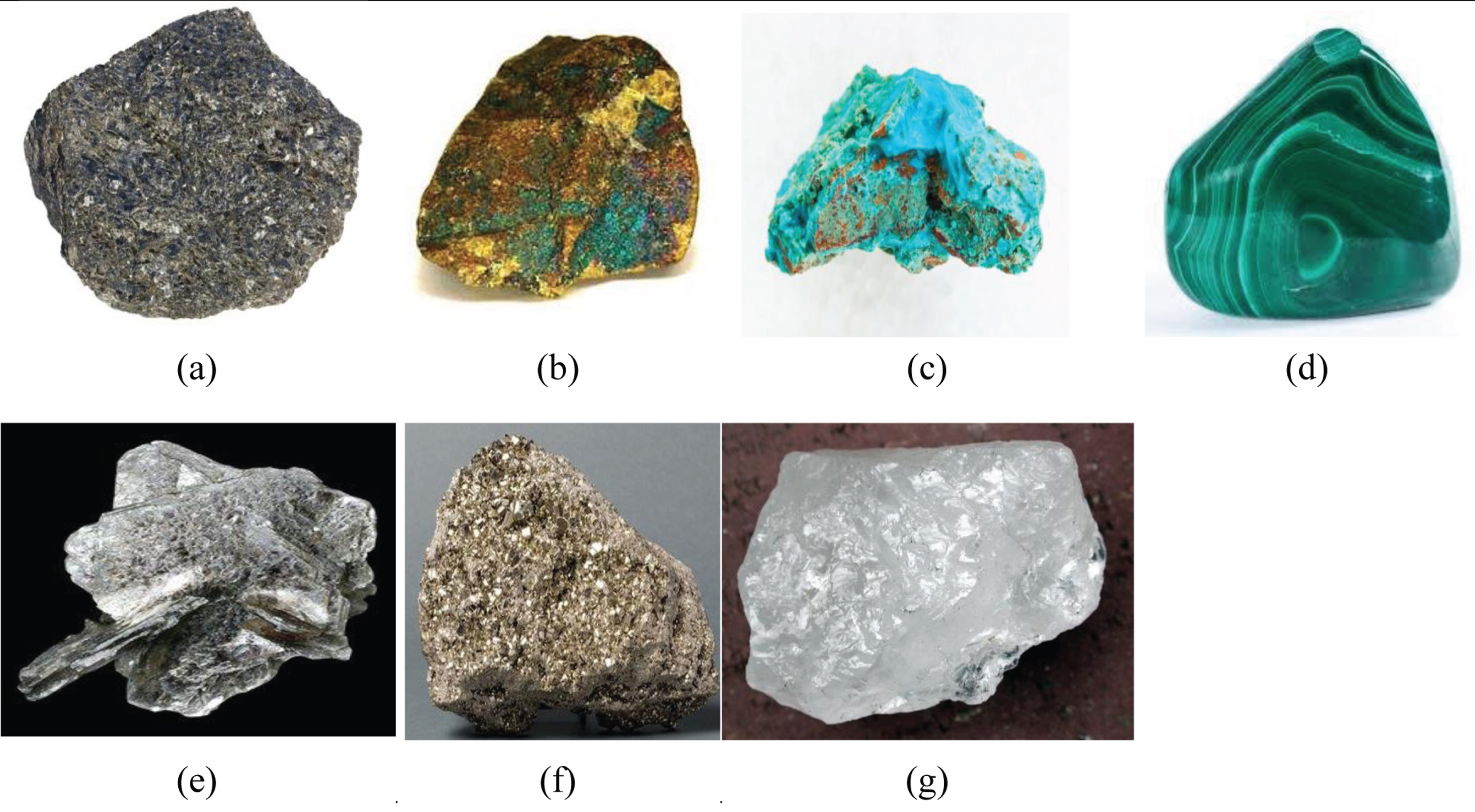
Hand Specimen Mineral Images (a) Biotite (b) Bornite (c) Chrysocolla (d) Malachite(e) Muscovite (f) pyrite (g) quartz.

OPEN IN VIEWER

Table 1

Dataset of hand specimen mineral images

Minerals	No. of Images
Biotite	68
Bornite	173
Chrysocolla	163
Malachite	235
Muscovite	77
Pyrite	98
Quartz	142

OPEN IN VIEWER

Table 2

Nine possible classification models

Pretrained Network	Feature fusion	Classification
model
Alexnet	Fc6 and Fc7	Classifier 1
	Fc7 and Fc8	Classifier 2
	Fc6 and Fc8	Classifier 3
VGG16	Fc6 and Fc7	Classifier 4
	Fc7 and Fc8	Classifier 5
	Fc6 and Fc8	Classifier 6
VGG19	Fc6 and Fc7	Classifier 7
	Fc7 and Fc8	Classifier 8
	Fc6 and Fc8	Classifier 9

3.2 Methodology

Identifying minerals in the field needs to be solved with difficulties. Traditional methods necessitate a high level of skill and are prone to errors. Deep learning approaches can solve challenges and give easy and effective mineral recognition methods. On the other hand, existing procedures primarily exploit minerals’ features under a microscope and emphasize a manual feature extraction pipeline. Deep learning with bi-layer feature fusion uses hand specimen photos to recognize seven different types of minerals. Alexnet’s fc6, fc7, and fc8 feature levels and vgg16 and vgg19 include three feature layers. Other models have only one feature layer, except for these three pre-trained CNN models. As a result, only Alexnet, vgg16, and vgg19 support multi-layer feature fusion. On Alexnet, vgg16, and vgg19, bi-layer feature fusion is demonstrated with various feature combinations. The proposed strategy is depicted in Fig. 2.

OPEN IN VIEWER

Fig. 2

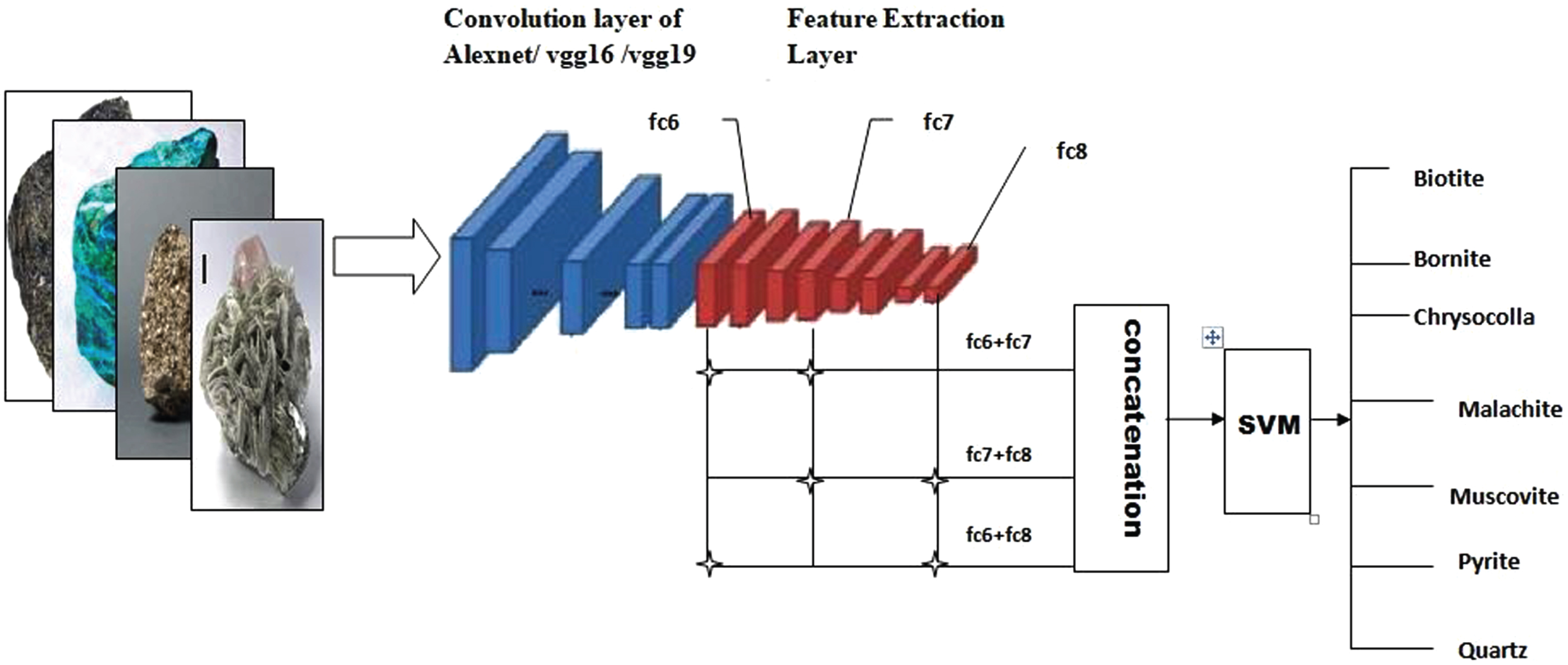
Bi-layer feature fusion for Mineral Recognition.

With the introduction of the above proposed framework, nine possible classification models have resulted. The possible bi-layer feature fusions are fc6 + fc7, fc7 + fc8, and fc6 + fc8. Further, these three feature fusions are applied to Alexnet, VGG16, and VGG19. So, there are nine classification models for the recognition of minerals, detailed in Table 1.

The fc6 & fc7 have 4096 features, and the fc8 has 1000 features. After the fusion of the two-layer, the resulting feature vector’s dimension is enhanced. The fc6 + fc7 have (4096 + 4096=) 8192, fc7 + fc8 have (4096 + 1000=) 5096 and fc6 + fc8 have (4096 + 1000=) 5096 number of features. The enhanced feature vector is fed to SVM for classification. The SVM is used here because of its error correcting and one-vs-all mapping approach, which enhances the classification accuracy compared to SoftMax did in pre-trained model.

The proposed framework for mineral recognition is executed in HP Pavilion core i5, Windows 10, 8GB RAM in MATLAB 2021a platform. The performance of all nine classification models is evaluated in terms of accuracy, sensitivity, specificity, precision, FPR, F1 score, MCC, and kappa score. In addition, the performance of Alexnet, vgg16, and vgg19 in three combinations of feature fusion, i.e., fc6 + fc7, fc7 + fc8, and fc6 + fc8, are recorded in Table 3.

It is observed from Table 3 that the bi-layer fusion of fc6 + fc7 performed better compared to fc7 + fc8 and fc6 + fc8. Again, among three CNN models in all three bi-layer fusion combinations, Alexnet is better than VGG16 and VGG19. Further, the confusion matrix of all possible nine classification models is illustrated. Figure 3 shows the confusion matrix resulting from the bi-layer fusion, i.e., fc6 + fc7; similarly, Figs. 4 and 5 shows the resulting confusion matrix of bi-layer fusion of fc7 + fc8 fc6 + fc8, respectively. Overall, using hand specimen images, the Alexnet with fc6 + fc7 performed well in recognizing seven kinds of minerals.

OPEN IN VIEWER

Fig. 3

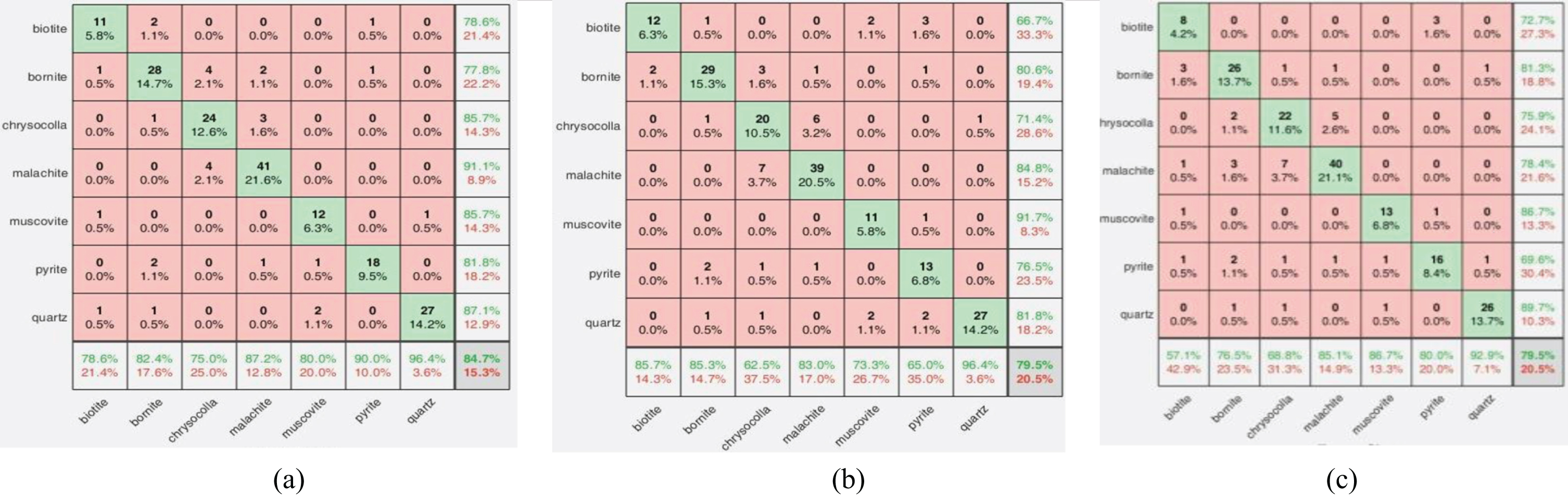
Confusion matrixes of bi-layer fusion of fc6 and fc7 (a) Alexnet (b) VGG16 (c) VGG19.

OPEN IN VIEWER

Fig. 4

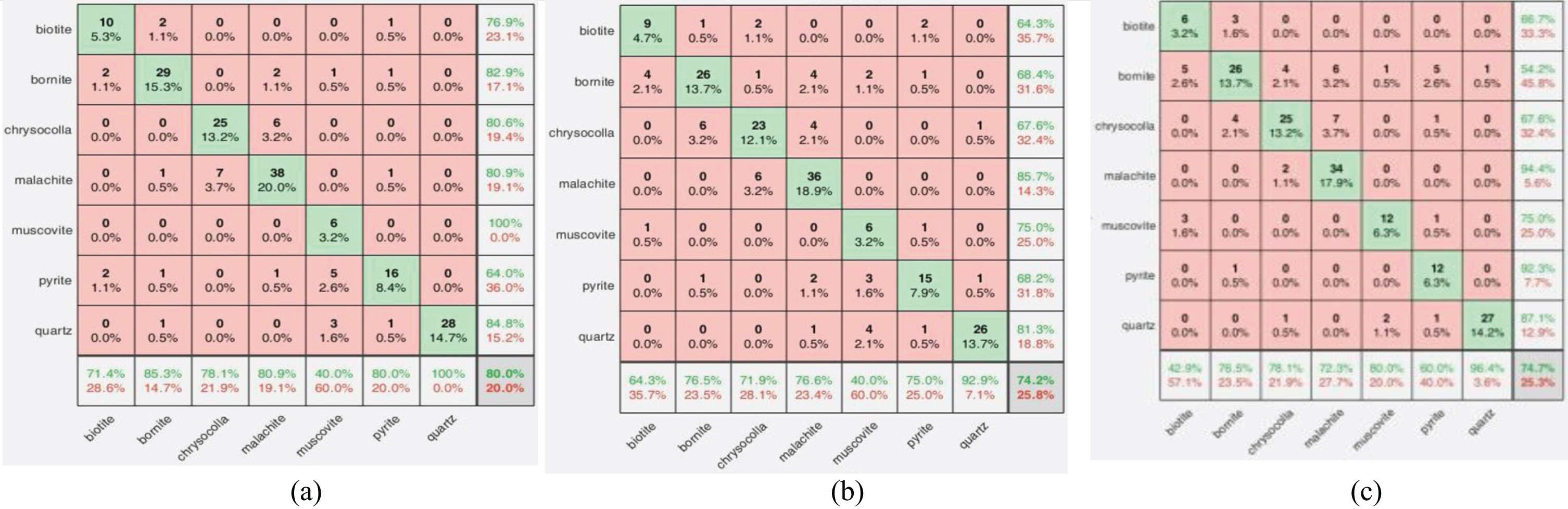
Confusion matrixes of bi-layer fusion of fc7 and fc8 (a) Alexnet (b) VGG16 (c) VGG19.

OPEN IN VIEWER

Fig. 5

Confusion matrixes of bi-layer fusion of fc6 and fc8 (a) Alexnet (b) VGG16 (c) VGG19.

Figure 3 (a), i.e., confusion matrix of Alexnet using bi-layer feature fusion of fc6 + fc7, shows that the true classification rate of each mineral ranges from 77.8% to 91.1%. In previous work [22], each mineral’s true classification rate ranges from 55.8% to 91.7%. Recently, another work [31] reported on mineral classification based on a deep-learning model. Both photos of mineral hand specimens and the Mohs hardness scale are utilized here. When the mineral image and hardness were used together, this model had an accuracy of 89% and 71.2% when only the mineral image was used. The Mohs Hardness Scale is a helpful tool for identifying minerals. The relative resistance to scratching of a mineral is assessed by scratching it against another substance of known hardness on the Mohs Hardness Scale [28]. Specialized test kits are required to assess the mineral’s Mohs hardness [29, 30]. As a result, considering Mohs hardness is not justified for a completely automated approach. With simply the usage of hand specimen mineral photographs, the proposed work outperformed the state-of-the-art.

Mineral recognition in mines site is a challenging task. Collecting mineral slices and installing the microscope in the mineral site is difficult. Here, an automated solution is provided to recognize minerals using hand specimen images. The bi-layer feature fusion technique is adapted to improve accuracy by enhancing the feature vector dimension. The performance of three bi-layer feature fusions, i.e., fc6 + fc7, fc7 + fc8, and fc6 + fc8, in three CNN models, i.e., Alexnet, VGG16, and VGG19, are carried out. The Alexnet with feature fusion of fc6 + fc7 provides the best result with an accuracy of 84.23%. Further, the true classification rate of each seven kinds of minerals ranges from 77.8% to 91.1%, which is better than the state-of-art. This result implies that the work is in the correct direction and helpful for geologists.

Declaration

Consent for publication

No third-party material was used.

Availability of data and materials

The data and materials will make available on request with valid reason.

Competing interests

Authors do not have any competing interests towards the publication of this article.

Funding

This research work is not funded by any institution or organization.

Author contributions

Prabira Kumar Sethy and Santi Kumari Behera both equally contributed to data collection, analysis, model design, and drafting of the manuscript.