
Abstract
Skin disease is currently considered to be one of the most common diseases in the globe. Most of the human population has experienced it at some point but not all skin illnesses are as severe as others. There are some diseases that are symptomless or show fewer symptoms. Skin cancer is a potentially fatal outcome of serious skin illnesses that might develop if they are not detected in time. Due to the fact that medical professionals aren’t always quick or reliable enough to make a proper diagnosis. There is a hefty price tag attached to employing sophisticated equipment. Therefore, we propose a system capable of classifying skin diseases using deep learning approaches, such as CNN architecture and six preset models including MobileNet, VGG19, ResNet, EfficientNet, Inception, and DenseNet. Acne, blisters, cold sores, psoriasis, and vitiligo are some of the most often seen skin conditions, thus we scoured the web resources for relevant photographs of these conditions. We have applied data augmentation methods to extend the size of the dataset and include more image variations. In the validation dataset, we achieved an accuracy rate of approx 99 percent, while in the test dataset; we achieved an accuracy rate of approx 90 percent. Our proposed method would help to diagnose skin diseases in a faster and more cost-effective way.
Keywords
Introduction
Based on algorithms inspired by the human brain’s structure and operation, deep learning is a subset of machine learning. This concept is well known as artificial neural networks. From driverless cars to face detection, everywhere, deep learning is working as a key technology. Digital assistants (Google Assistant, Alexa, Cortana, etc.), voice-enabled TV/AC/Fan remotes, credit card fraud detection, and so on are all powered by it. Deep learning is the best technology for image, text, and sound-based classification problems. In these fields, researchers can yield good accuracy and performance using deep learning techniques. It sometimes exceeds human-level performance. Deep learning is majorly used in Artificial Intelligence applications and helps to improve automation, and it can solve analytical and physical problems without any human intervention. Basically, artificial neural networks, or deep learning neural networks, are inspired by the functionality of the human brain through data inputs, weights, and biases that are used to train neural networks. These components work together to aid the model in effectively recognizing, classifying, and describing objects inside the data element. The nodes that make up a neural network are collectively referred to as neurons. These artificial neurons help to create the basic structure of biological neurons of the human brain.
A neuron’s value is encoded as a number (e.g. 1.8, 5.4, 42.7, 1.2, etc.). Weights are the numerical value that helps to realize the connection between the neurons.
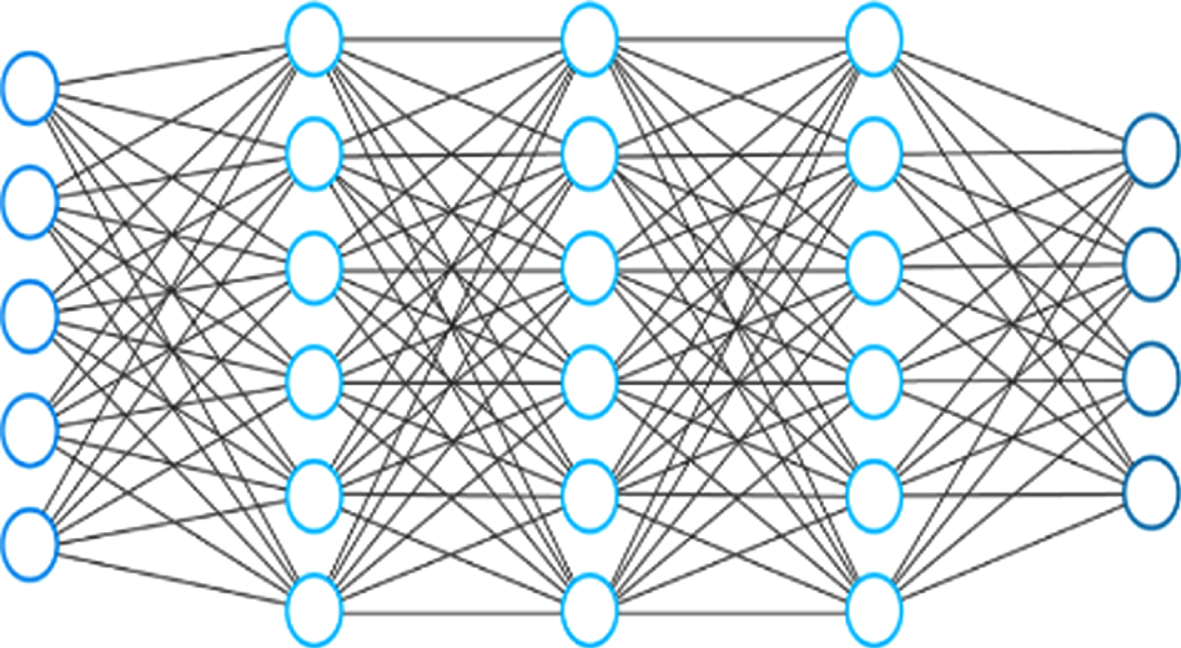
An artificial feed forward neural network.
There are several layers in basic Neural Network architecture. The input layer is the first one. The neural network’s learning process feeds the input data to the input layer. A similar number of neurons make up the input layer’s neurons.
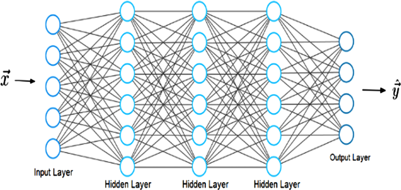
A feed-forward neural network’s structure.
Finally, the output layer is at the end of the stack. It is the output vector y that reflects what the neural network was able to predict. The neuron’s entrance vector values are reflected in the output layer’s value. These visible layers, which include the input and output, are so named. The data is fed into the deep learning model at the input layer, and it is the model’s output at the output layer that makes the final prediction or classification. Between the input and output layers are the Hidden layers. With the help of an activation function, the artificial neurons here produce an output from a series of weighted inputs. The weight matrix represents the weight between the two neural network layers.
For a given feature vector x, the neural network generates a prediction vector. The h vector is shown below.
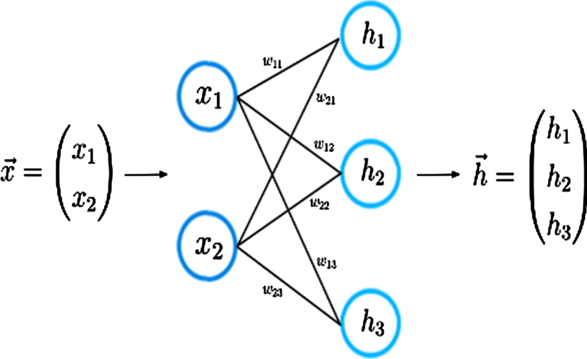
Forward propagation.
Forward propagation is another term for this process. Our input vector x is multiplied by the weight matrix W to get the dot product. Again, it will produce a vector which we call it z.
In order to get a prediction vector, we’ll need to apply an activation function to the input vector, z. Sigma is the letter used to symbolize the activation function. From z to h, it is a nonlinear mapping performed by this nonlinear function.
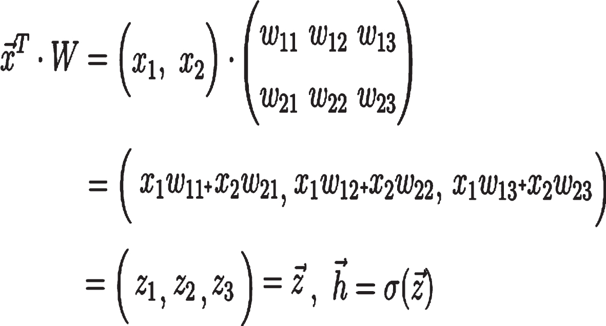
Equations for forward propagation.
Using the forward and backward propagation of information, a neural network may make predictions and then correct itself if it is wrong. In this way, the algorithm improves over time.
Our contribution to the proposed method is shown below. Our model structure is very simple and easily understandable. The previously mentioned pre-trained models have complex architectures. During the training of those models, huge computation costs and time were required. But with its simple architecture, it is showing good accuracy compared to the other models. Less training time is required for our model. Less computational cost is required.
In order to acquire a rapid overview of recent work on skin disease classification using deep learning and machine learning methodologies, we meticulously analyzed several academic publications. Deep learning and image processing-based algorithms have been proposed by certain researchers to determine the type of skin illness. We would go over some of the tactics that have been reported in the literature in this piece.
Color images are used to build an artificial neural network model for dermatological disease detection, according to [1]. The initial step is to use color image processing techniques, k-means clustering, and color gradient algorithms to locate the damaged skin area. The second aim is to utilize ANN to classify the six different kinds of skin disorders. The first stage’s average accuracy is 95.99 percent, while the second stage’s average accuracy is 94.016 percent.
The authors [2] have placed a special emphasis on various segmentation strategies that can improve image processing and improve the accuracy of Melanoma detection. They’ve presented a Melanoma diagnosis tool for dark skin that uses a specialized algorithm and incorporates a selection of Melanoma photos from various sources.
In [3] authors demonstrated the accuracy of the SVM-based approach in the diagnosis of melanoma, basal cell carcinoma (BCC), nevi, and seborrheic keratosis (SK).
An eczema severity scale was created by MD. Nafiul Alam et al. [4]. The system is split into three parts. It will first detect effective skin segmentation. Then, using color, texture, and boundaries, extract a set of features. Finally, using the SVM algorithm, the severity of eczema will be determined.
Computer vision and machine learning are used by VB Kumar et al. in their study [5] to diagnose six distinct kinds of skin disorders. This system has a 95% accuracy rate.
We have investigated some existing common methods in the deep learning arena before proposing our suggestion.
With the Convolutional Neural Network (CNN) or ConvNet [6], Yann LeCun has created a multi-layer image processing and object detection system. CNNs are frequently used to discover anomalies, identify satellite pictures, interpret medical imaging, forecast time series, and find anomalies. Convolution Layer, Rectified Linear Unit (ReLU), Pooling Layer, and Fully Connected Layer are the CNN layers. Data processing and feature extraction are handled by these layers.
A form of Recurrent Neural Network (RNN), called LSTMs (Long Short-Term Memory Networks) [7], may learn and remember long-term relationships. The default nature of LSTMs is to recall past information for lengthy periods of time. For LSTMs, it is possible to store information across time. They’re useful for time-series prediction since they recall previous inputs. The four interacting layers of an LSTM have a chain-like structure that allows them to communicate uniquely. Other than time-series forecasts, LSTMs are used for speech recognition and music composition, and pharmaceutical research.
The LSTM outputs can be used as inputs in the current phase using RNNs [8], which have connections that produce directed cycles. The present phase now takes the LSTM output as an input. It has internal memory, which allows it to remember previous inputs. The most prevalent applications are image captioning, natural language processing, time-series analysis, handwriting recognition, and machine translation.
GANs (Generative Adversarial Networks) [9] are generative deep learning algorithms that produce new data instances that resemble the training data. Generators and discriminators are both components of GANs, and they work together as a system that can learn how to generate false data. GANs have become increasingly popular in recent years. Dark matter research can benefit from using them to better astronomical photography. To replicate previous 2D visuals in 4K or greater resolutions, video game makers typically utilize GANs to upscale their low-resolution images using image training.
Feed-forward neural networks that use radial basis functions (RBFNs) are known as RBFNs. There are three layers to these algorithms: an input, a hidden layer, and a final output layer. RBFNs employ the similarity of the input to the examples in the training set to solve classification problems. It consists of a layer of neurons and an input vector that feeds into the input layer.
MLPs (Multilayer Perceptrons) [11] is a type of feed-forward neural network that consists of multiple layers of Perceptrons with activation functions. MLPs are made up of two layers: an input layer and an output layer, both of which are fully connected. They have the same number of input and output layers, but there might be numerous hidden layers. MLPs are largely used in the creation of software for speech, image, and machine translation.
Self-Organizing Maps (SOMs) were created by Professor Teuvo Kohonen [12]. For data visualization, it employs self-organizing artificial neural networks to reduce data dimensionality. Data visualization is a solution to the problem of individuals struggling to visualize high-dimensional data. It facilitates the understanding of this multidimensional data.
Deep Belief Networks (DBNs) [13] are multi-layered stochastic and latent variable generative models. Hidden units refer to the binary values of the latent variables. They are made up of a series of Boltzmann Machines that are connected. Each RBM layer can communicate with both the levels above and below it. Image recognition, video recognition, and motion capture data are the most frequently used applications.
Geoffrey Hinton [14] created Restricted Boltzmann Machines (RBMs). RBMs are probabilistic neural networks that can learn from a probability distribution across a set of inputs. This approach to deep learning is frequently employed for dimensionality reduction, regression, classification, feature learning, collaborative filtering, and topic modeling. The visible and hidden units of RBMs are made up of two sections. All of the visible units are linked to all of the ones that are hidden. It also has a bias unit that is connected to all of the visible and hidden units but has no output nodes.
Autoencoders [15] is a type of feed-forward neural network that has the same input and output. Geoffrey Hinton created autoencoders to handle unsupervised learning difficulties in the 1980 s. Autoencoders are neural networks that have been programmed to copy information from one layer to the next. Autoencoders are utilized in numerous areas, such as popularity prediction, drug development, and image processing.
We have also studied some most popular predefined deep learning models.
Mobile applications were in mind when the MobileNet idea [16] was developed. Depth-wise Convolutions were employed in the MobileNet project. When compared to a network with regular convolutions of the same depth in the nets, it reduces the number of parameters, resulting in lightweight deep neural networks. Google has made the CNN-based MobileNet technology open-source. As a result, this is a good place to start when it comes to training our ultra-compact and lightning-fast classifiers.
The VGG19 [17] model is merely a variation of the VGG model. There are 19 layers in all, with 16 convolution layers, 3 fully connected layers, 5 MaxPool layers, and 1 SoftMax layer.
Shaoqing Ren et.al. were the first to introduce ResNet [18]. It is one of the most well-known and effective deep learning models. It is mostly inspired by VGG19’s architecture. Its design is made up of a 34-layer simple network with shortcut and skip connections placed on top.
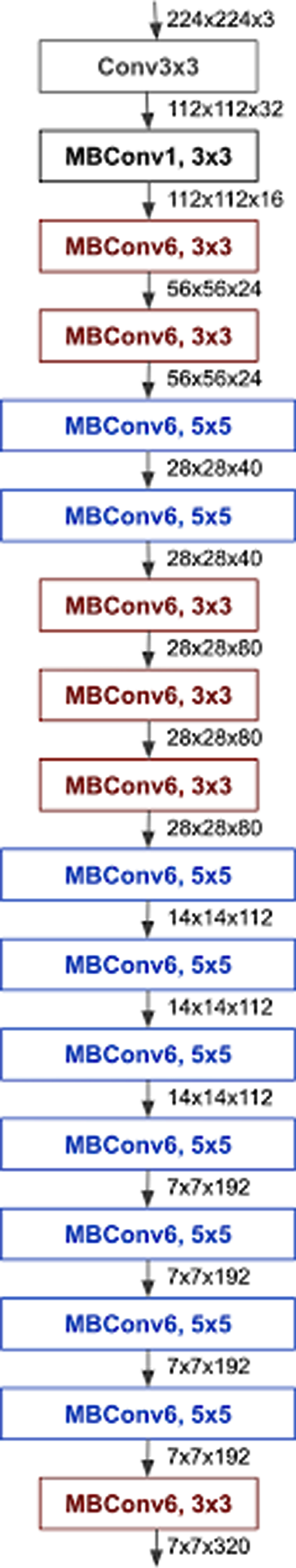
EfficientNet [19] is based on a convolutional neural network design that scales all depth/width/resolution dimensions with a compound coefficient. The baseline network plays an important role in the effectiveness of model scaling. To get a family of models, we aim to scale up the baseline network.
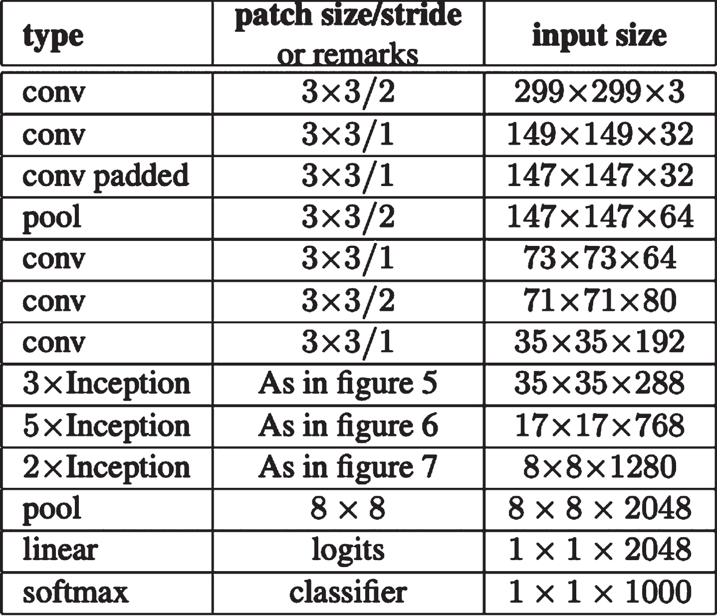
Inception-v3 [20] is a convolutional neural network design from the Inception family that tries to transmit label information lower down the network with enhancements such as Factorized 7 x 7 convolutions, Label Smoothing, and an auxiliary classifier.
A DenseNet [21] is a convolutional neural network with dense connections between layers created using Dense Blocks. Each layer takes extra inputs from all preceding levels and passes on its feature maps to all subsequent layers to retain the feed-forward nature.
Our proposal for skin disease classification using deep learning
To develop the deep learning-based skin disease detection system, we have followed the following steps:
Data collection
We have worked on only five skin diseases which are acne, blister, cold sore, psoriasis, and vitiligo. We have collected images of these diseases from various web resources. JPEG, JPG, and PNG image formats are considered for image selection.
Data augmentation
We apply data augmentation techniques to increase the size of the dataset and make variations of images. Here, we have performed various operations like rotation_range, brightness_range, shear_range, zoom_range, fill_mode, horizontal_flip, vertical_flip, rescale, data_format, validation_split, and dtype. Then we iterate the function for 10 times to get a good variety of images.
Data preprocessing and enhancement
It is a very important step as the model performance mostly depends on the type and quality of the dataset. To do this we have used the preprocessed input of MobileNetV2 as pre-processing function. Here we got a NumPy array of data type float32. We have resized all the images as 224 x 224. This image dimension is standard for most of the pre-trained models.

Train, Ttest and validation data generation
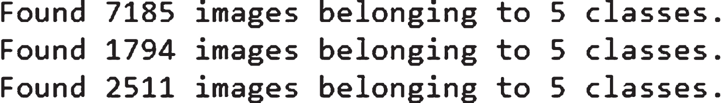
After data preprocessing, first we split the data into Train data and Test Data randomly. We have used 20% of the train data for validation. There are 7185 train images, 1794 validation images and 2511 test images.
As our problem is categorical type so we select the class mode as categorical. Flow_from_direactory does auto labeling of the image data classes. So, no manual labeling is required.

Model building
We have used the Convolutional Neural Network (CNN) algorithm which learns automatically and divides the provided data into the levels of prediction and gives accurate results very fastly.
In the case of classifying images, CNN stands out among all alternative algorithms. It has some special characteristics like Shared Weights, Sparse Connectivity, and Pooling layer which are the best for extracting the best features from image data. To use CNN, we have used Keras Sequential API.
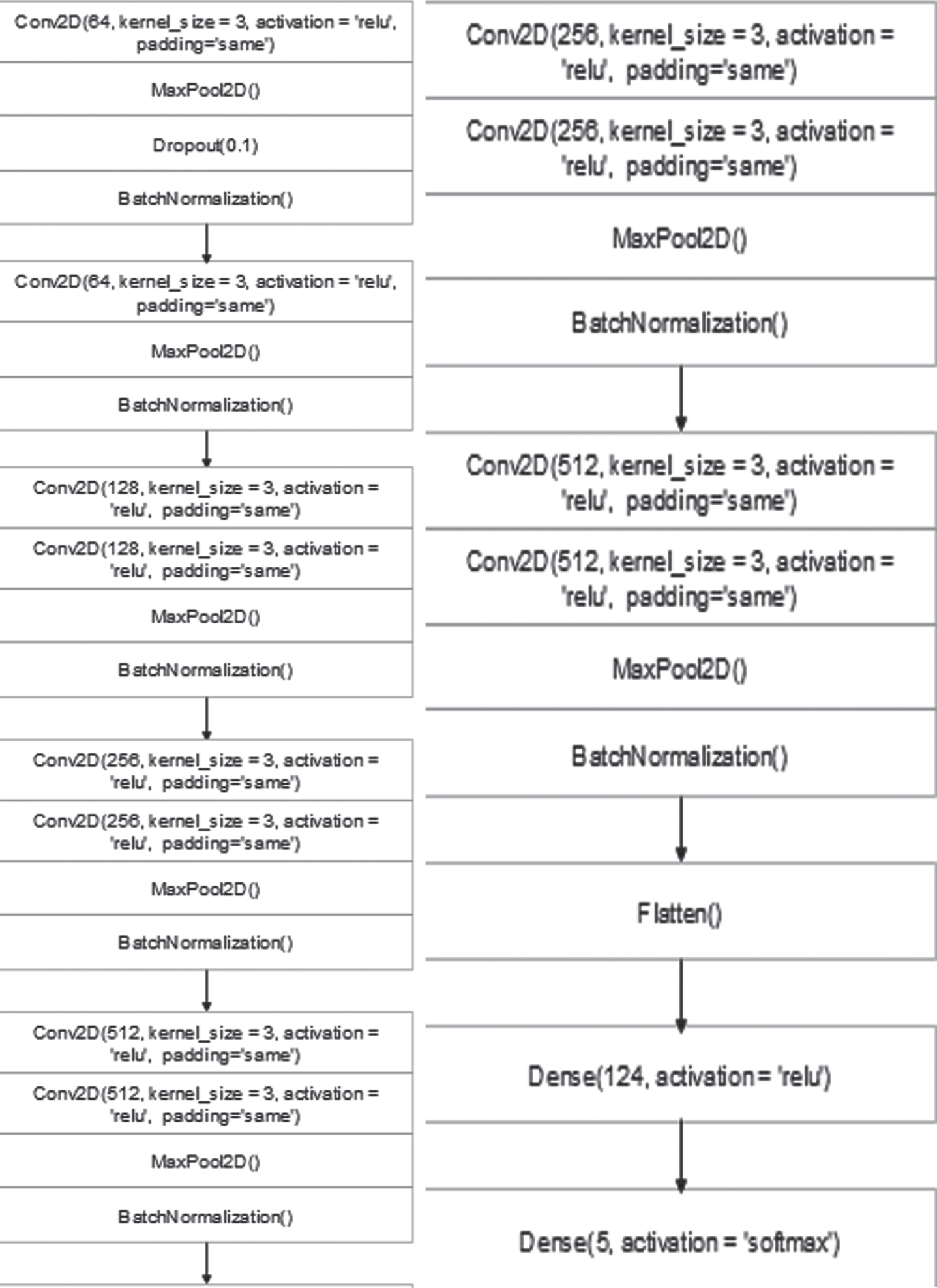
Our model consists of 1 input layer, 6 hidden layers, 1 flatten layer, and 1 output layer. The kernel is set to 3. ReLu has been used as an activation function in our model. Input shape is [224,224,3]. Padding is set to ‘Same’. After each layer Maxpool layer and Batch Normalization has been used. In the output layer, we have used the ‘Softmax’ activation function as our data is categorical in nature.
We define categorical cross entropy as our system is based on a multi-class classification problem. Next we have chosen ‘Adam’ as optimizer as it has so many advantages compared to other optimizers.

After that we have selected ‘Accuracy’ as the metric function which involves evaluating the performance of the system. We keep the default Learning Rate(LR) of the ‘Adam’ optimizer which is 0.001.
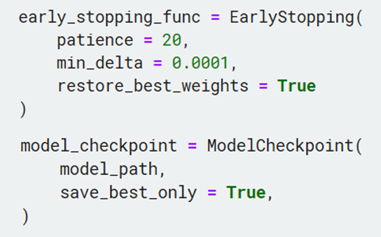
We have created to call back functions: EarlyStopping and ModelCheckpoint. When the monitored matric stops improving, EarlyStopping stops the training. We set the patience as 20, min_delta as 0.0001 and restore the best weight. ModelCheckPoint helps to save the best model weights.
We have created to call back functions: EarlyStopping and ModelCheckpoint. When the monitored matric stops improving, EarlyStopping stops the training. We set the patience as 20, min_delta as 0.0001 and restore the best weight. ModelCheckPoint helps to save the best model weights.

Finally, we train our model for 100 epochs.

Using of pre-defined models
MobileNet
The MobileNet model is designed for use in mobile applications. Depth wise Convolutions has been used in MobileNet. Compared to the network with regular convolutions with the same depth in the nets, it reduces the number of parameters which results in lightweight deep neural networks. The Depthwise separable convolution is made from two operations. One is Depthwise convolution and another is Pointwise convolution.
MobileNet is a CNN based system which was open-sourced by Google. Therefore, this gives an excellent starting point for training our classifiers which are insanely small and insanely fast.
VGG19
VGG19 is just a variant of the VGG model. It consists of 19 layers where 16 layers are convolution layers, 3 layers are Fully connected layers, 5 MaxPool layers and 1 SoftMax layer. Here are the VGG19 Layers:

ResNet
Residual Network (ResNet) was first introduced by Shaoqing Ren, Kaiming He, Jian Sun, and Xiangyu Zhangis. It is one of the famous and most successful deep learning models. It is mainly inspired by the architecture of VGG19. Its architecture consists of a 34-layer plain network in which the shortcut connection or the skip connections are added. Here is the architecture of ResNet:

EfficientNet
EfficientNet is based on a convolutional neural network architecture that can uniformly scale all dimensions of depth/width/resolution using a compound coefficient. The effectiveness of model scaling relies on the baseline network heavily. To obtain a family of models we basically try to scale up the baseline network.
InceptionV3
Inception-v3 is a convolutional neural network architecture from the Inception family which tries to propagate label information lower down the network by including improvements like Factorized 7 x 7 convolutions, Label Smoothing, and an auxiliary classifier.
DenseNet
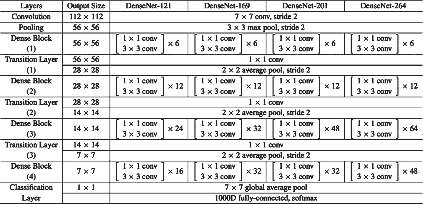
A DenseNet is based on the convolutional neural network which utilizes dense connections between layers, through Dense Blocks. Here each layer obtains additional inputs from all preceding layers and passes on its feature-maps to all subsequent layers to preserve the feed-forward nature. Here is the DenseNet Architecture:
Results and discussion
Results
Each model is evaluated based on its level of accuracy and its level of loss. In this case we have considered Validation Accuracy and Test Accuracy for the evaluation purpose.
Our model
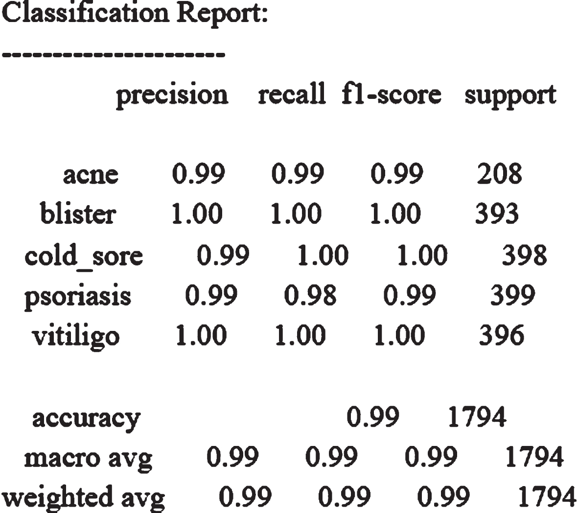
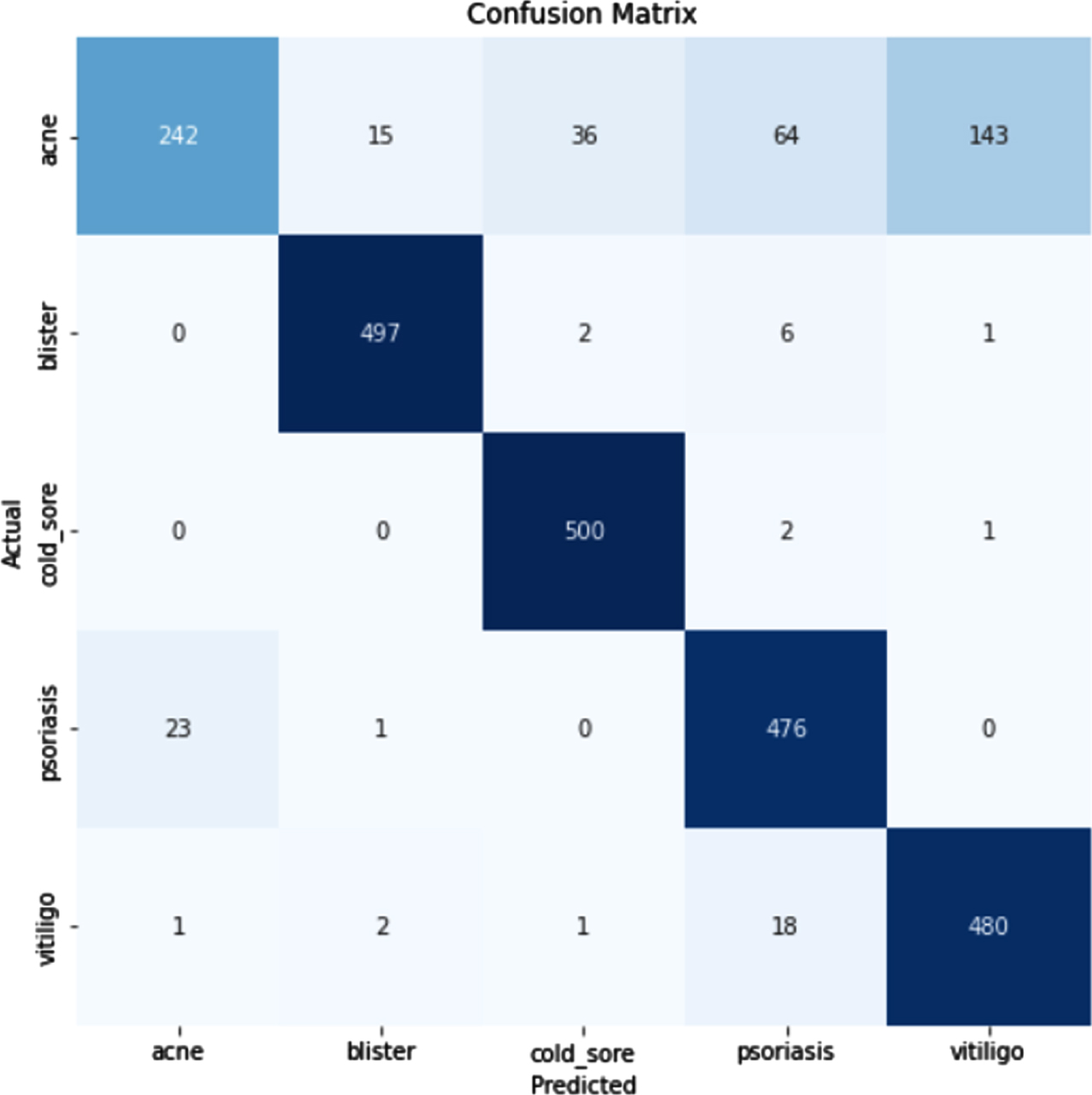
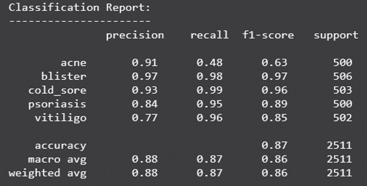
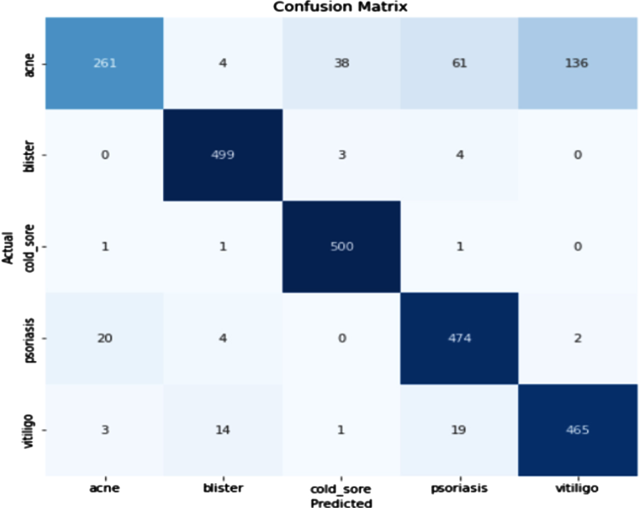
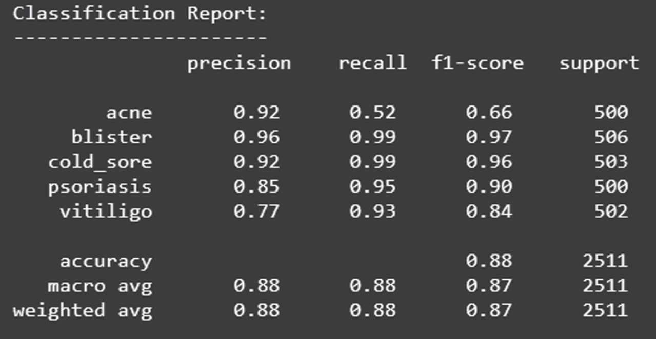
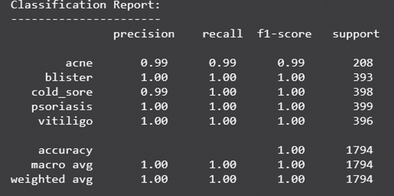
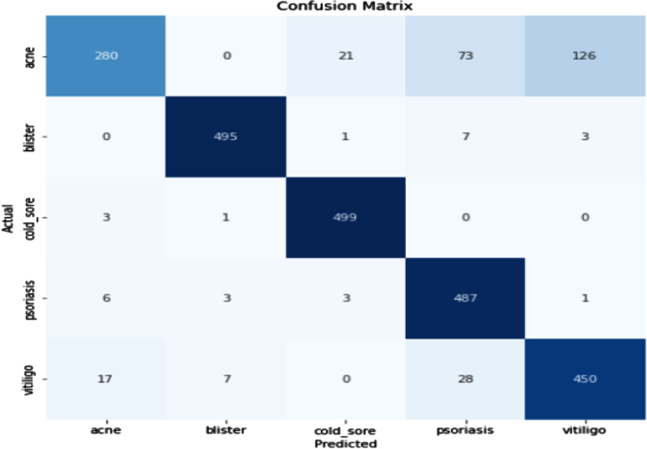
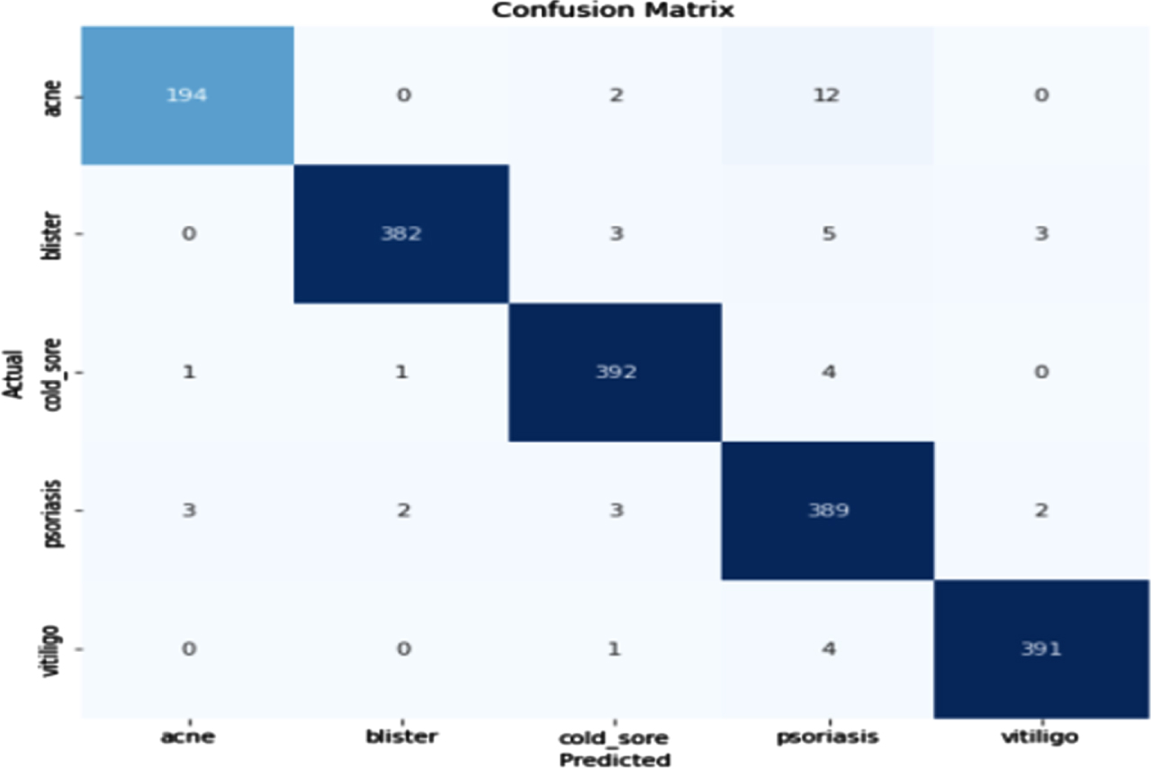
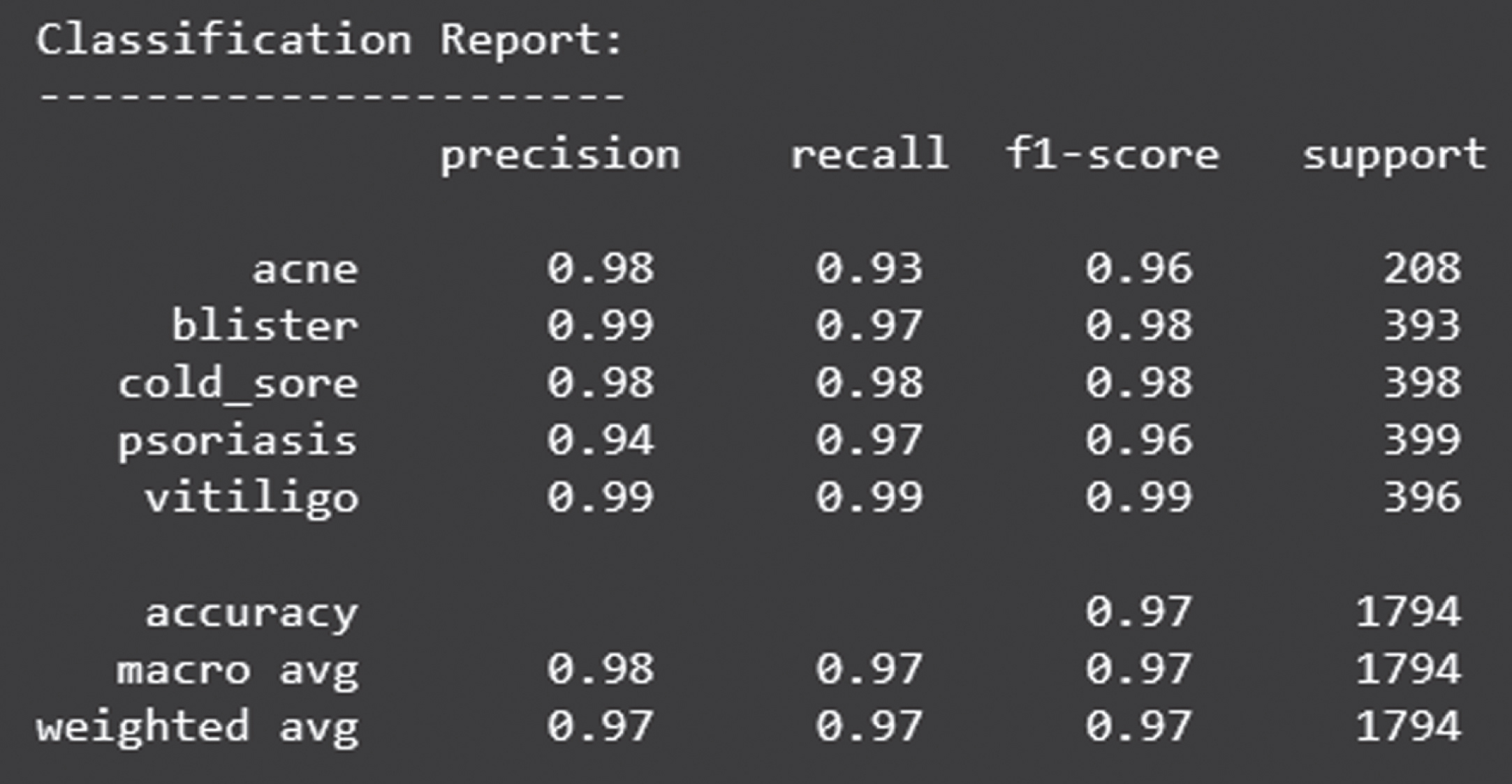
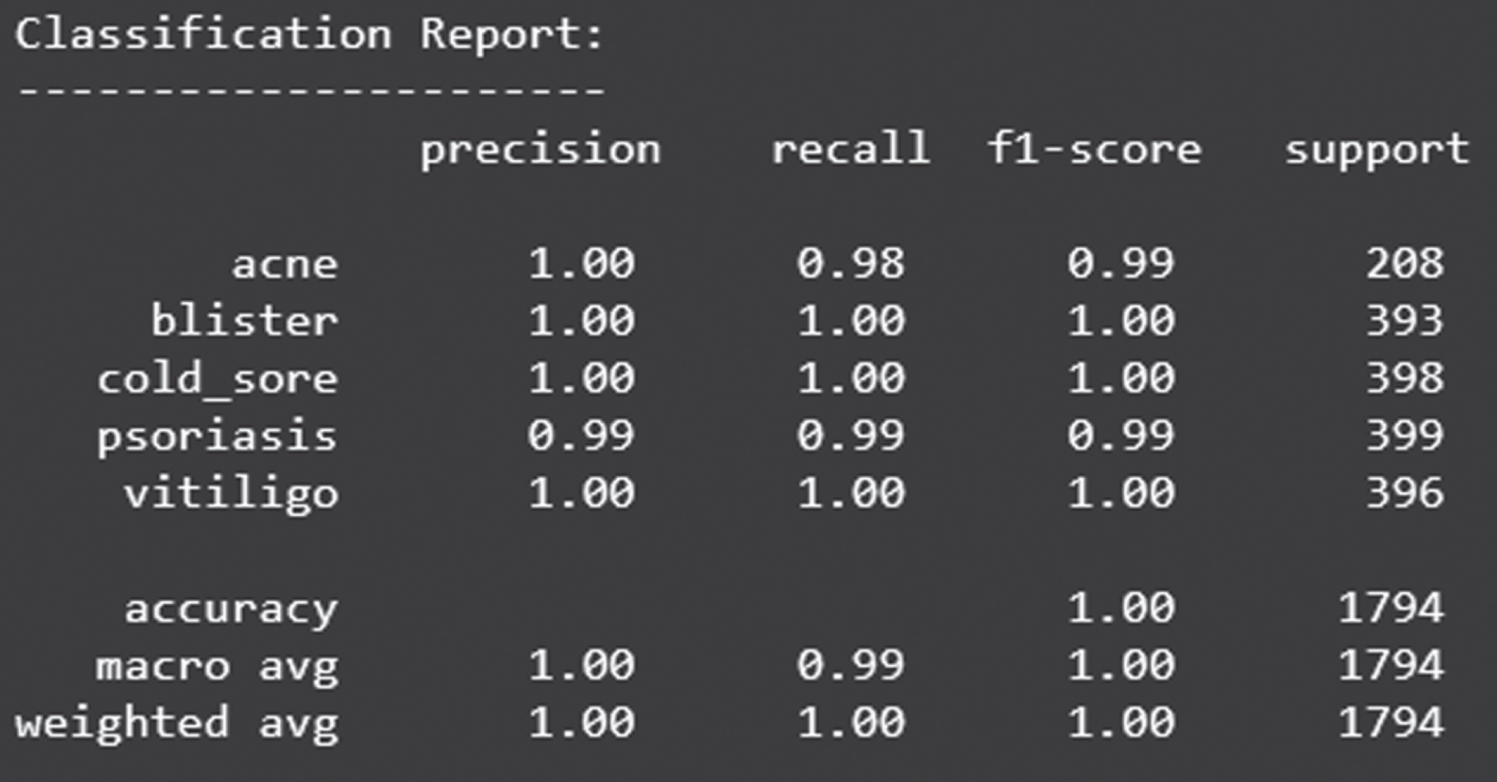
Figure 5 shows the loss obtained by the proposed model. Figure 6 depicts the Confusion Matrix, whereas Fig. 7 depicts the Classification report for Test Accuracy. The Confusion Matrix is depicted in Fig. 8 and the Classification report for Validation Accuracy is depicted in Fig. 9.

Training and validation loss graph
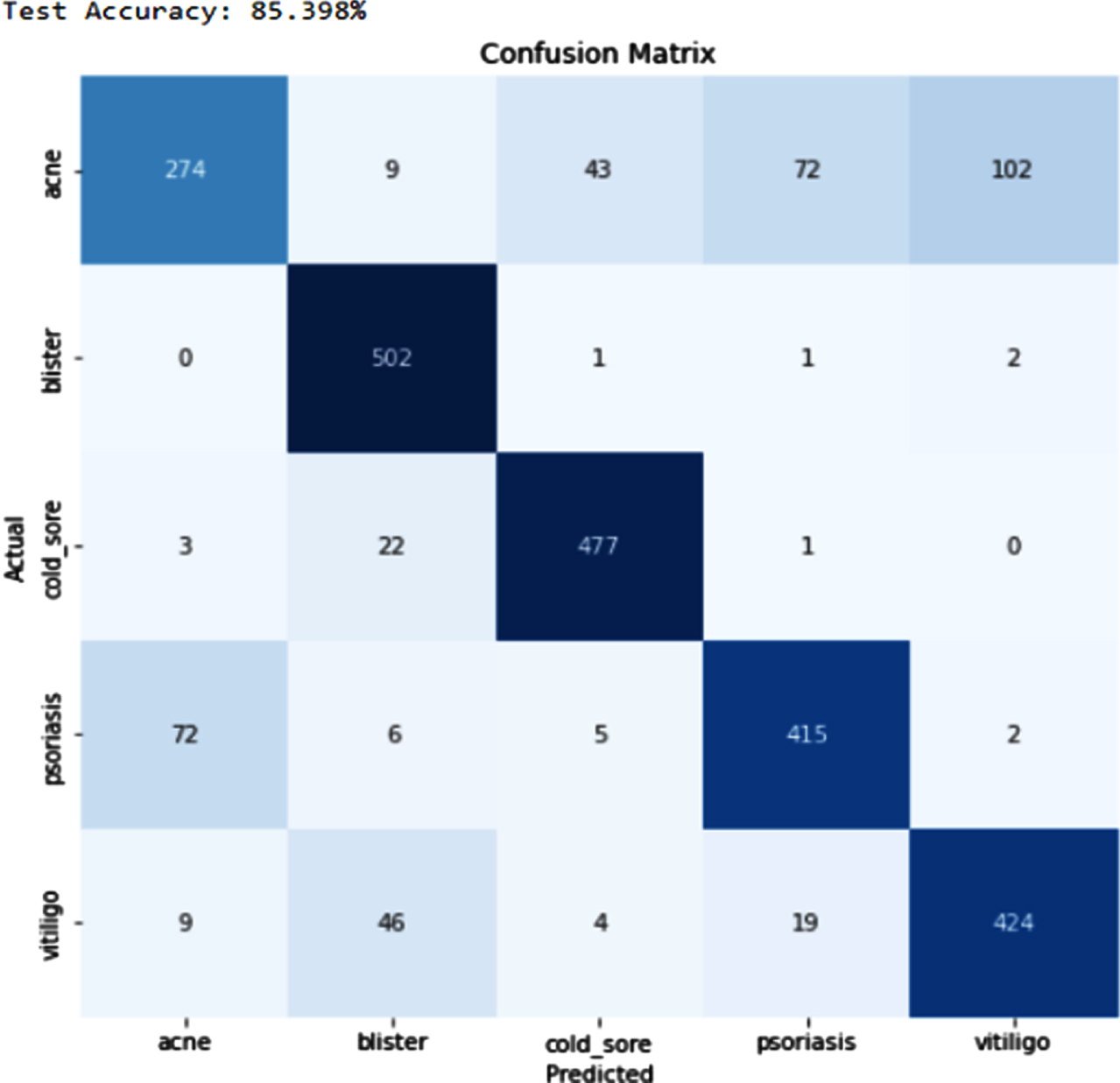
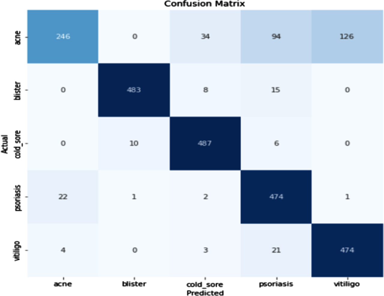
Test accuracy and confusion matrix
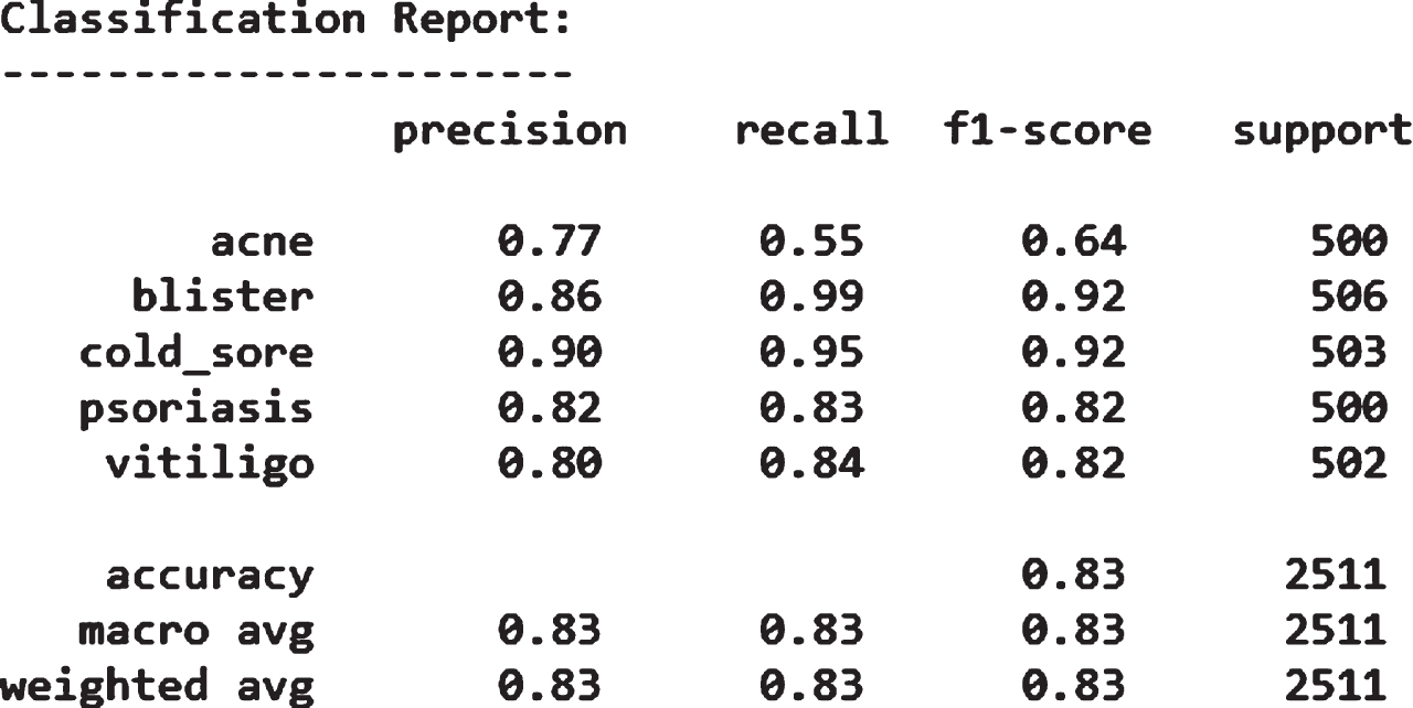
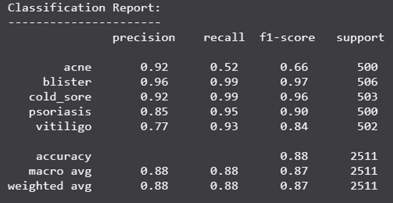
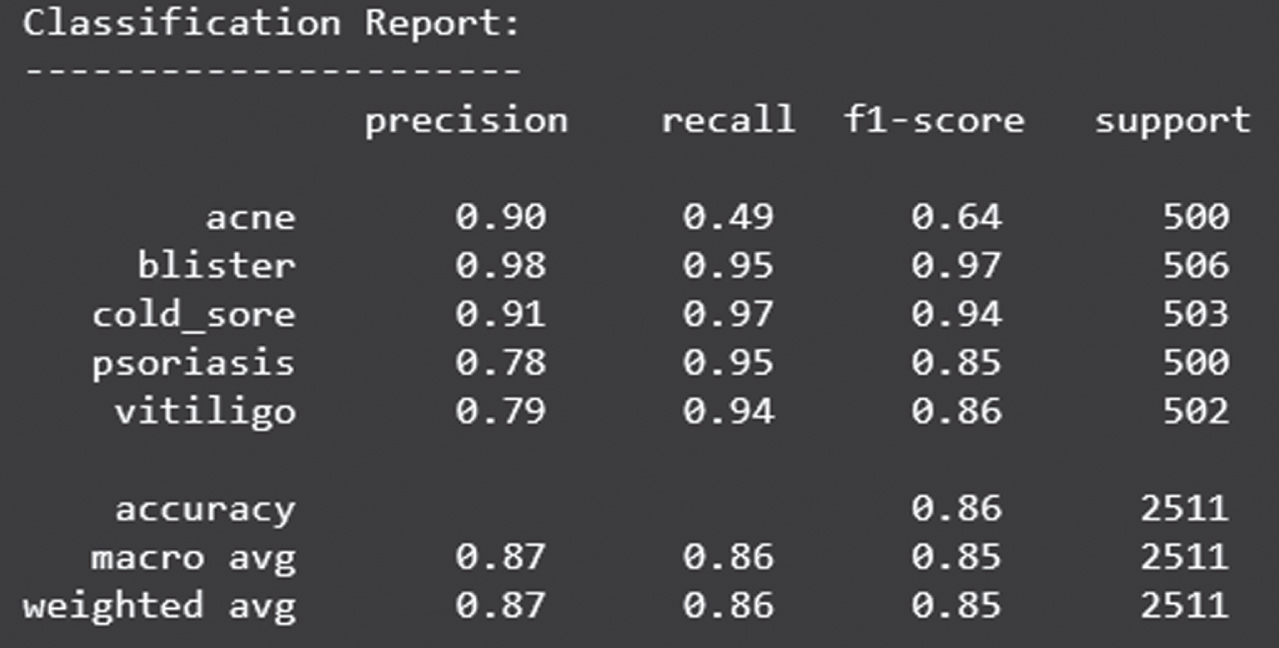
Classification report of test accuracy
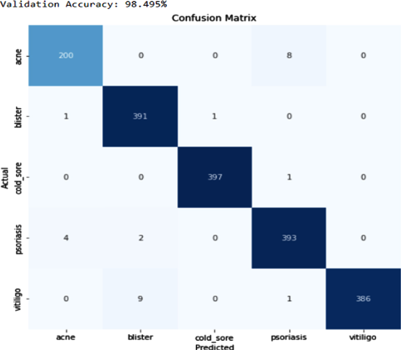
Validation accuracy and confusion matrix

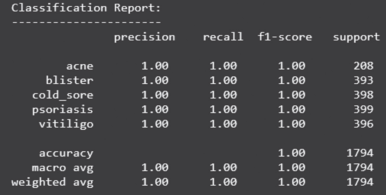
Classification report of validation accuracy
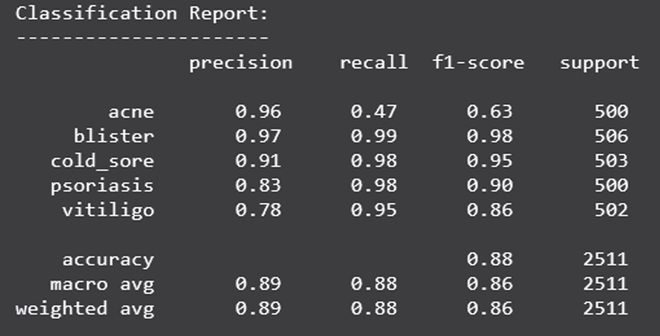
Figure 10 shows the loss obtained by MobileNet model. Figure 11 depicts the Confusion Matrix, whereas Fig. 12 depicts the Classification report for Test Accuracy. The Confusion Matrix is depicted in Fig. 13 and the Classification report for Validation Accuracy is depicted in Fig. 14.

Training and validation loss graph of MobileNet

Test accuracy and confusion matrix

Classification report of test accuracy

Validation accuracy and confusion matrix
Classification report of validation accuracy
Figure 15 shows the loss obtained by VGG19 model. Figure 16 depicts the Confusion Matrix, whereas Fig. 17 depicts the Classification report for Test Accuracy. The Confusion Matrix is depicted in Fig. 18 and the Classification report for Validation Accuracy is depicted in Fig. 19.

Training and validation loss graph of VGG19
Test accuracy and confusion matrix
Classification report of test accuracy

Validation accuracy and confusion matrix

Classification report of validation accuracy
Figure 20 shows the loss obtained by ResNet model. Figure 21 depicts the Confusion Matrix, whereas Fig. 22 depicts the Classification report for Test Accuracy. The Confusion Matrix is depicted in Fig. 23 and the Classification report for Validation Accuracy is depicted in Fig. 24.

Training and validation loss graph of ResNet
Test accuracy and confusion matrix
Classification report of test accuracy

Validation accuracy and confusion matrix
Classification report of validation accuracy
Figure 25 shows the loss obtained by EfficientNet model. Figure 26 depicts the Confusion Matrix, whereas Fig. 27 depicts the Classification report for Test Accuracy. The Confusion Matrix is depicted in Fig. 28 and the Classification report for Validation Accuracy is depicted in Fig. 29.

Training and validation loss graph of EfficientNet
Test accuracy and confusion matrix
Classification report of test accuracy

Validation accuracy and confusion matrix
Classification report of validation accuracy
Figure 30 shows the loss obtained by InceptionV3 model. Figure 31 depicts the Confusion Matrix, whereas Fig. 32 depicts the Classification report for Test Accuracy. The Confusion Matrix is depicted in Fig. 33 and the Classification report for Validation Accuracy is depicted in Fig. 34.

Training and validation loss graph of InceptionV3
Test Accuracy and confusion matrix
Classification report of test accuracy
Validation accuracy and confusion matrix
Classification report of validation accuracy
Figure 35 shows the loss obtained by DenseNet model. Figure 36 depicts the Confusion Matrix, whereas Fig. 37 depicts the Classification report for Test Accuracy. The Confusion Matrix is depicted in Fig. 38 and the Classification report for Validation Accuracy is depicted in Fig. 39.

Training and validation loss graph of DenseNet

Test accuracy and confusion matrix
Classification report of test accuracy

Validation accuracy and confusion matrix
Classification report of validation accuracy
Train, Validation, and Test Accuracies of the Models:

From the Figs. 40 41, we can observe that MobileNet shows very good performance on both test and validation data. All the models have above 80% accuracy for both the cases. InceptionV3’s little bit less in case of validation data. But it has not that much effect. Our model test accuracy is little less which can be increased in future work. No overfitting and underfitting cases are observed for any models.

Comparison of test accuracies of the models.
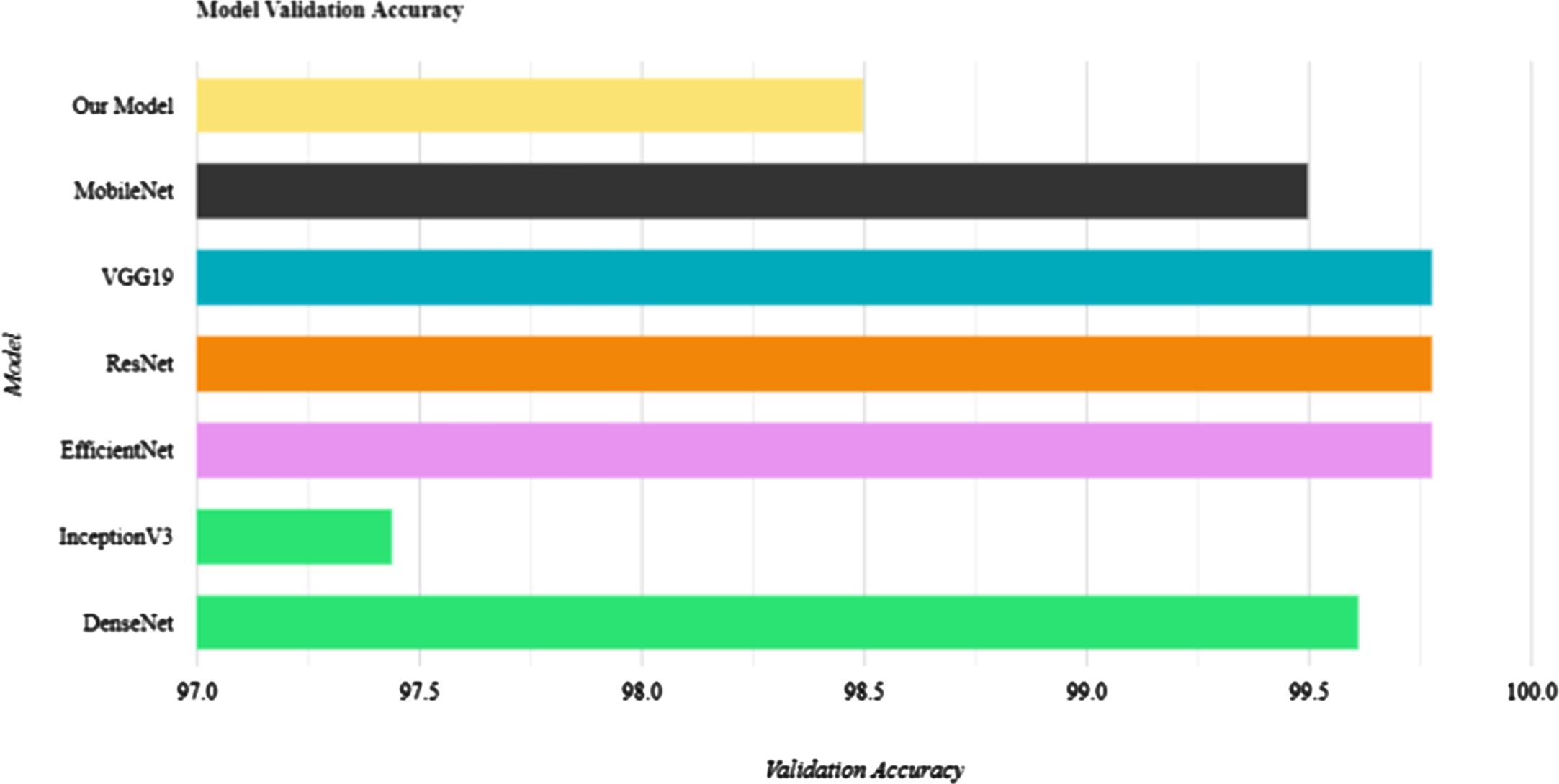
Comparison of Validation Accuracies of the Models.
Skin Diseases are the fourth most common reason for human illness. For the diagnosis of skin diseases, we have presented a robust and automated system which will help in treatment of skin diseases in a more effective and cost-effective way. This technique will aid in diagnosing skin disorders without the assistance of a dermatologist. In future with detection, we also want to incorporate some medication procedures for quick relief.
Funding resources
There are no Funding Resources and Funding Supports are available for the said work.