Application of deep learning to multivariate aviation weather forecasting by long short-term memory

Abstract

Weather forecasts are essential to aviation safety. Unreliable forecasts not only cause problems to pilots and air traffic controllers, but also lead to aviation accidents and incidents. This study develops a long short-term memory (LSTM) integrating both multiple linear regression and the Pearson’s correlation coefficients to improve forecasting. A numerical dataset of 10 weather features (sea pressure, temperature, dew point temperature, relative humidity, wind speed, wind direction, sunshine rate, global solar radiation, visible mean, and cloud amount) is applied on every calendar day in a year to train and validate the LSTM for temperature forecasting. It is shown that data standardization is necessary to rescale the data to improve training convergence and reduce training time. In addition, feature selection by multiple linear regression and by Pearson’s correlation coefficients are shown effective to the forecast accuracy of the LSTM. By selecting only the sensitive features (sea pressure, dew point temperature, relative humidity and relative humidity), the temperature forecasting errors can be reduced from RMSE 4.0274 to 2.2215 and MAPE 23.0538% to 5.0069%. LSTM deep learning with data standardization and feature selection is effective in forecasting for aviation safety.

Keywords

Deep learning aviation weather long short-term memory weather forecasting

1 Introduction

Accurate weather forecasting is essential for aviation safety. The unpredictable nature of aviation weather has posed many challenges to scientists and pilots worldwide. Poor weather affects aircraft operations, increases operating cost, and causes accidents. New methods and technologies can predict atmospheric states. Because the atmosphere is continuous, multidimensional, and dynamic, considerable computational power is required to solve equations that predict weather conditions. Numerical weather prediction (NWP) was first proposed by Richardson a century ago [1] to simulate the physical equations of the atmosphere and oceans based on current weather conditions and predict future weather. However, NWP still has fundamental problems. The partial differential equations governing the chaotic nature of the atmosphere are impossible to solve analytically. Consequently, NWP cannot compute numerical results quickly. Operational forecasters are still required to make subjective forecasts in the absence of effective tools. The quality of a weather forecast is often limited by insufficient data on regional characteristics and past weather events. Finding a cost-effective forecasting strategy has become a primary focus in aviation.

Some researchers have argued that deep learning using big data such as weather images, satellite images, and long-term time-series variables can be used to forecast weather. Long short-term memory (LSTM) is a type of recurrent neural network (RNN) in deep learning that is used to investigate long dependency and sequential problems. However, when applied to geosciences, difficulties arise due to the continuously increasing sophistication of environmental models [2]. Vlachas et al. [3] demonstrated that an RNN with backpropagation has excellent forecasting abilities and can capture the dynamics of reduced-order systems. Bocquet et al. [4] proposed the Bayesian statistics method to learn long time series data from observations of geophysical flows. Geer [5] verified the equivalencies between four-dimensional variational data assimilation and an RNN. Kashinath et al. [6] demonstrated that machine learning can also facilitate emulating, downscaling, and forecasting weather. The RNN in machine learning is seldom applied in aviation meteorology due to its inability to store information in the long term. Additionally, RNNs have been demonstrated to have vanishing and exploding gradients in which errors accumulate during updates (i.e., iterations).

Sangiorgio and Dercole [7] demonstrated that an LSTM architecture can maintain good performance when the number of time lags included in the input differed from the actual embedding dimension of the dataset. Hong et al. [8] adapted an LSTM to very short-term weather forecasting. With the development of deep learning, LSTMs are now well-suited to classifying, processing, and predicting the long-term time series data. Furthermore, Xu et al. [9] proposed a generative adversarial network (GAN) with LSTM model by combining the former’s generating ability with the latter’s forecasting ability to capture the evolution of weather systems. Zhu et al. [10] used deep learning to show that the multifactor prediction model was more stable than the single factor in the prediction of airport visibility. Zhang et al. [11] proposed multimodal fusion to predict weather visibility by combining numerical prediction with a satellite image to improve visibility prediction. Deng et al. [12] and Meng et al. [13] used the LSTM model to predict visibility, but the result had a time delay problem and could only achieve a prediction accuracy.

In weather forecasting, Salman et al. [14] proposed a forecasting model that builds upon LSTM to predict weather data at an Indonesian airport. Vlachas et al. [15] proposed a hybrid architecture to extend the forecasting capability of LSTM. Elsaraiti and Merabet [16] proposed a prediction model based on LSTM to forecast the wind speed values of multiple time steps. He et al. [17] proposed using LSTM to forecast wind power and meet the demands of power system economic dispatching and day-ahead market purchasing power. However, none is on aviation meteorology in Taiwan. This study aims to apply an LSTM to model time series data and to increase the accuracy of temperature forecasting by selecting important features. For aviation safety, if various weather phenomena can be accurately classified and processed successfully, accurate prediction is achievable for decision making.

2 Architecture of long short-term memory

An RNN considers information from the prior input that may influence the present input and output. A typical RNN uses feedback loops to carry information over time, and has a memory ability that allows the network to store previous information. However, the problems of long-term temporal dependencies are difficult to solve by standard RNN shown in Fig. 1(a), where the output of previous time step h_t - 1 is dependent on the input x_t - 1 with hyperbolic tangent (tanh) as an activation function to model nonlinearity. In theory, an RNN shall have the ability to handle arbitrary long-term dependencies, while in practice, it still suffers from the problem of vanishing and exploding gradients because the output of the previous layer is used as the input for the further layers. The network continues to multiply with the same exact weight (w) multiple times, and the gradient becomes less and less with each multiplication by multiplying a smaller weight [18]. LSTM is a type of RNN capable of analyzing long-term dependent problem and preventing the gradient problems. An LSTM has feedback connections composed of three gates, as shown in Fig. 1(b). The gates update and control the cell states C_t and the hidden states h_t. The cell state C_t is to model longer memory that stores and loads information of previous time step and encodes a kind of aggregation of data from the previous time step. It is a kind of conveyor belt, running straight down the entire chain and carrying the information from the previous time step to the next time step. The hidden state h_t is to model short-term memory, encodes a kind of characterization of the previous time step data, and it is more concerned with the recent time step. Because of the ability to memorize and forget information, an LSTM can train single data and multisequential data as well.

The three gates are the forget gate f_t, input gate i_t and output gate o_t with sigmoid (σ) and tanh activation functions. The sigmoid function is to calculate a set of scalars to prevent vanishing/exploding gradients and the tanh is to transform the data into a normalized encoding of the data. The forget gate is a sigmoid function to decide if the output h_t-1 of the previous time step and the input x_t of this time step should be kept or not.

Fig. 1

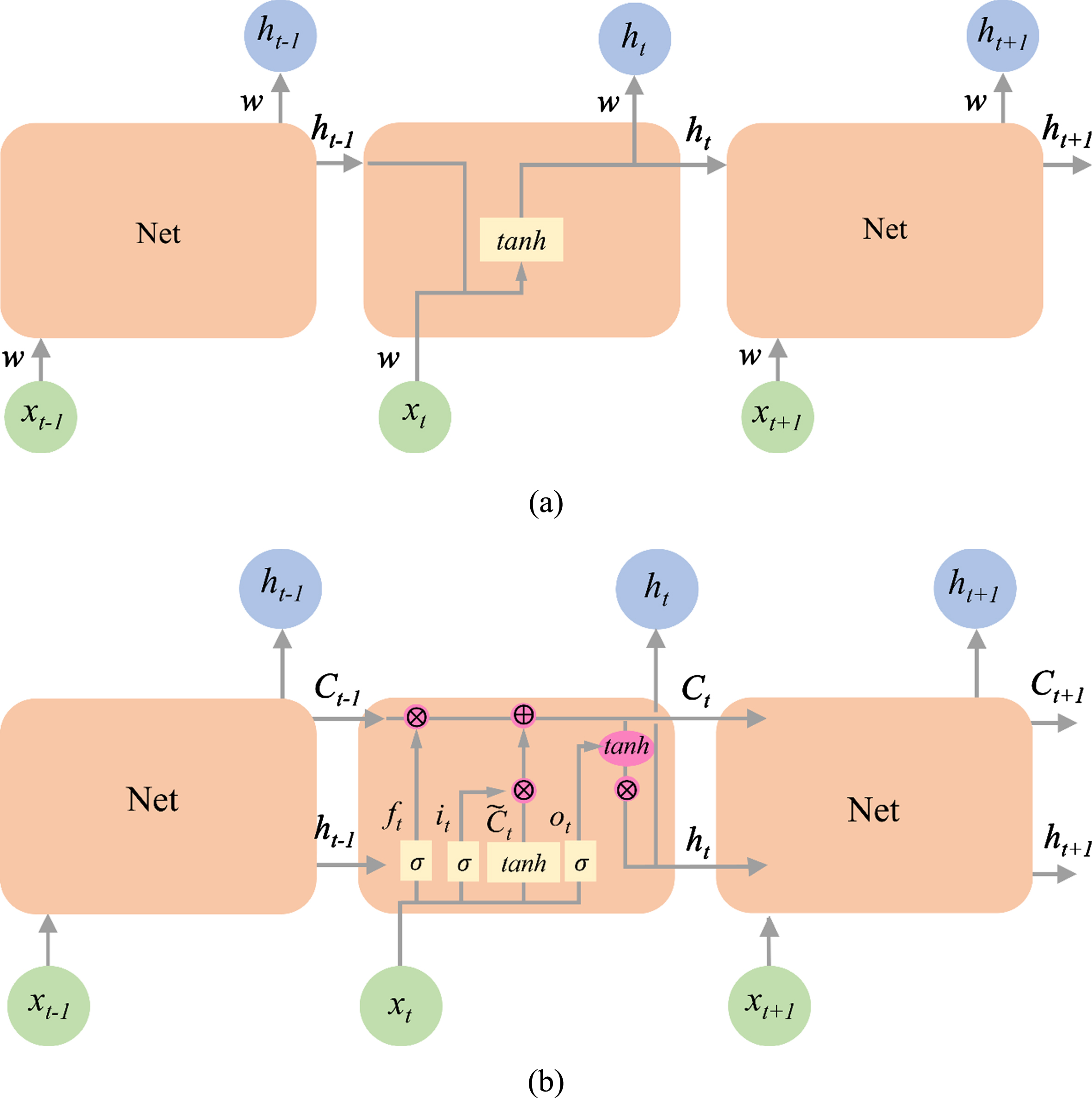
(a) The structure in a standard RNN contains a single layer, where Net represents a chunk of neural network, x is the input, h is the output, and tanh is the tangent function. The subscript t - 1, t, and t + 1 are the previous, present, and next time step, respectively, and w is the weight. (b) The structure in an LSTM contains four interacting layers by using feedback connection, where ⊗ is the pointwise multiplication, ⊕ is the pointwise addition, σ is the sigmoid function, f_t is the forget gate, i_t is the input gate, o_t is the output gate and ${\tilde{C}}_{t}$ is the cell state.

$f_{t} = σ [(w_{f} (h_{t - 1} + x_{t}) + b_{f}],$ (1) where w_f and b_f are the weight and offset value of the forget gate. The input gate has two steps to decide whether the storage of new information is needed in the cell state C_t. The input gate decides the probability of input of which should be updated and generates a value between [0,1] by a sigmoid function. The meaning of 0 and 1 is completely deleted and passed, respectively. Then, the tanh function creates a value between [–1,1] for the new candidate of cell state ${\tilde{C}}_{t}$ , which is generated to add to the cell state C_t $i_{t} = σ [(w_{i} (h_{t - 1} + x_{t}) + b_{i}],$ (2) ${\tilde{C}}_{t} = \tanh [(w_{c} (h_{t - 1} + x_{t}) + b_{c}],$ (3) where w_i and b_i are the weight and offset value of the input gate i_t, and w_c and b_c are the weight and offset value of the new candidate cell state ${\tilde{C}}_{t}$ . The next step is to update the new cell state C_t by multiplying the previous cell state C_t-1 with the forget gate f_t and adding a new candidate of cell state $i_{t} * {\tilde{C}}_{t}$ , where * denotes convolution operation and the dimension corresponds to the number of training features in LSTM $C_{t} = f_{t} * C_{t - 1} + i_{t} * {\tilde{C}}_{t} .$ (4)

In the output gate, the previous hidden state h_t-1 and the present input x_t pass through a sigmoid function to generate an output gate. Then, the output gate o_t goes through a newly modified cell state C_t with tanh function, which means the last step controls the information encoded in the cell state C_t to be the input to the next hidden state h_t+1. The output or prediction can be expressed as $o_{t} = σ [(w_{o} (h_{t - 1} + x_{t}) + b_{o}],$ (5) $h_{t} = o_{t} * \tanh (C_{t}),$ (6) where w_o and b_o are the weight and offset of the output gate, h_t is the output of hidden state, representing short term memory and C_t is the cell state, representing long-term memory.

LSTM utilizes the three gates to compensate what RNN lacks in memorizing and forgetting the information. The forget gate f_t is to decide if the output of the previous time step and the input of the present time step should be kept or not. The input gate i_t is to quantify the importance of input, and a new candidate cell state ${\tilde{C}}_{t}$ is to control the information to be encoded into the cell state. The output gate o_t is to control the number of inputs for the next time step by encoding or filtering the information into the present time step. These three gates allow knowledge about the cell state and hidden state at every time step to address the vanishing gradient problem. Therefore, LSTM is often used to train long time series data such as weather forecasting because of its powerful learning capabilities [19].

3 Multivariate numerical data preprocessing

3.1 Data description

In this study, data were collected for 10 weather variables. Sea pressure (SP) was included due to its association with boundary layer inversions, radiative cooling at the water surface, clear skies, and the presence of anticyclones. An increase in SP, or persistently high values, indicates a synoptic situation conducive to fog formation. The dew point temperature (DP) and dry-bulb temperature can indicate the occurrence of fog. Environmental humidity is affected by wind and rainfall. Relative humidity (RH) also affects other climatic variables. Visibility measurements, such as the visibility mean (VM), provide short-term nowcasting guidance when the ambient air temperature approaches its dew point and mist begins to form. Total cloud amount (CA) is a prerequisite for fog formation and is determined by the occurrence of clear nocturnal skies. The sunshine rate (SR) is a climatological indicator of sunshine duration; it is used to measure the duration of sunshine during a given period (usually a day or a year) for a given location and is typically expressed as an average value over several years. Global solar radiation (GR) is the solar radiation that reaches the Earth’s surface without being diffused; atmospheric conditions can reduce direct beam radiation by 10% on clear, dry days and by 100% on overcast and humid days. Wind speed (WS) is a major determinant of fog; high wind speeds can dissipate mist before it forms into a thicker layer of fog, and low wind speeds allow turbulent mixing to circulate cool air and deepen the fog layer. Wind direction (WD) is an indicator of either the synoptic situation (i.e., long lead) or local conditions (i.e., short lead). Fog likelihood can be determined on the basis of both the WS and WD. For example, at a longer lead time, afternoon southeasterlies are usually indicative of a synoptic situation that is not conducive to fog. However, at a shorter lead time (e.g., during nocturnal periods), mild southeasterlies are symptomatic of katabatic drainage flow, which is often necessary for fog formation. Such weather information is cross-related. For example, air density is related to air temperature and pressure, and the air temperature is related to the DP and RH.

3.2 Data standardization

Raw data are often in large sets. Therefore, data preprocessing is necessary before deep learning and is also essential for handling missing, unsorted, off-scale, nonstationarity, and multicollinearity data to improve training convergence and reduce training time. In this study, the data include SP (hPa), temperature (°C), DP (°C), RH (%), WS (m/s), WD (°), SR (%), GR (MJ/m²), VM (km), and CA (0–10). The data vary vastly in terms of magnitude. In aviation, data are often differentiated; for example, in Taiwan, the SP is approximately 1013.25 hPa, but the temperature ranges between 9°C and 32°C. Therefore, preprocessing data by scaling is necessary for aviation weather predictions. Data preprocessing through z-score standardization is performed using the following equation: $x^{'} = (x - μ) / β,$ (7) where x is the original data, x′ is the new data after preprocessing, μ is the mean value of the data, and β is the standard deviation. Standardization has two benefits for training the model: improving the convergence speed and increasing the forecast accuracy. The gradient descent method is used to calculate the optimization during the construction of a deep learning model, but the data may not converge if the values vary vastly. For example, if the SP is in the range of [1001.3, 1029.1] and the DP is between [3.1, 26.1], then the effect of SP is likely to be much greater than that of DP. However, if the DP is more sensitive, then the off-scale data distort the forecast. Through data preprocessing, the convergence time of the gradient descent method can be reduced.

3.3 Feature selection

In this study, the data input into a model were called features. The predicted feature was called the response feature, and the remaining features for training LSTM were called predictor features. The collected data are often in substantial quantities, and some of the predictor features may not contribute significantly to the performance of the model. Therefore, using only predictor features can slow down the training process and cause the model to run slower. Moreover, the model may learn using irrelevant data and subsequently produce inaccurate forecasting results. Thus, only the essential predictor features should be used to train an optimal model. The method of selecting key predictor features is called feature selection.

Multiple linear regression is a statistical model that is used to predict the relationship between a dependent variable (response feature) and one or more independent variables (predictor features). Multiple linear regression can be used to identify a regression line that best describes the data, and the distances between the real and predicted values are the errors. The best-fit line has the lowest sum of squares of the errors. The correlation coefficient of the regression line describes the mathematical relationship between each independent variable and the dependent variable, and the P values for the correlation coefficients indicate whether these relationships are statistically significant. The significance level indicates the probability of rejecting the null hypothesis and is often set at 0.05 [20]. A P value that is greater than the significance level is nonsignificant, and the predictor feature is excluded.

Pearson’s correlation coefficient (ρ) is another means of feature selection used to determine the linear relationship between two features in data. A correlation coefficient of 1 indicates that for every positive increase in one feature, a positive increase of a fixed proportion occurs in the opposite feature. Conversely, a correlation coefficient of –1 indicates that for every positive increase in one feature, a negative decrease of a fixed proportion occurs in the opposite feature. A value of 0 indicates that for every increase, neither a positive nor negative increase occurs, and the two features are irrelevant. If 0.1 < ρ < 0.3 or –0.1 < ρ < -0.3, then the two features have a low intensity. If 0.3 < ρ < 0.5 or –0.3 < ρ < -0.5, then the two features have a medium intensity. If 0.5 < ρ < 1.0 or –0.5 < ρ < -1.0, then the two features have a high intensity [21, 22].

4 Temperature forecasting

4.1 Training options

In this work, the LSTM is trained by MATLAB on a 4 core Intel i5-1135G7 CPU @ 2.40 GHz and a NVIDIA GeForce MX350 graphics card with 20 GB RAM. The network using LSTM is shown in Fig. 2. A sequence input layer is applied to the LSTM layer with 500 hidden units for output. The hidden units are corresponding to the amount of information remembered between the time steps, and they can flexibly be set from a few dozen to a few thousand depending on the hardware resource. A fully connected layer is then used to map the output of the LSTM layer to a desired output, and the regression output layer is used to compute the mean square error loss. There are several options for training the LSTM. The initial learning rate is to control how much to change the model in response to the estimated error each time model w is updated. If the learning rate is too low, the training will take a long time. If the learning rate is too high, the training might reach a suboptimal or even diverge. For setting the training cycle, one epoch is when an entire data is passed forward and backward through the neural network only once. The learning rate schedule is to decrease the learning rate during training, ‘none’ means the learning rate remains constant throughout the training, and ‘piecewise’ means the software updates the learning rate every certain number of epochs by multiplying with a certain learning rate factor. The learning rate drop factor is a factor to drop the learning rate, specified as a scalar from 0 to 1 to apply to the learning rate every time a certain number of epochs passes. This option is valid only when the learning rate schedule training option is ‘piecewise’. The gradient threshold is set as a positive value. If the gradient exceeds the value of the gradient threshold, then the gradient is clipped to help prevent gradient explosion by stabilizing the training at higher learning rates and in the presence of outliers. In this study, the adaptive moment estimation algorithm [23, 24] is used as the training optimizer. The initial learning rate factor is 0.005, the maximum number of training epochs is 250, the learning rate schedule is set to ‘piecewise’, the learning rate drop factor is 0.2, and the gradient threshold is 1. After training the model with these options, a figure of training progress is used to confirm whether overfitting is performed or not. The testing data are then applied to predict by the LSTM.

Fig. 2

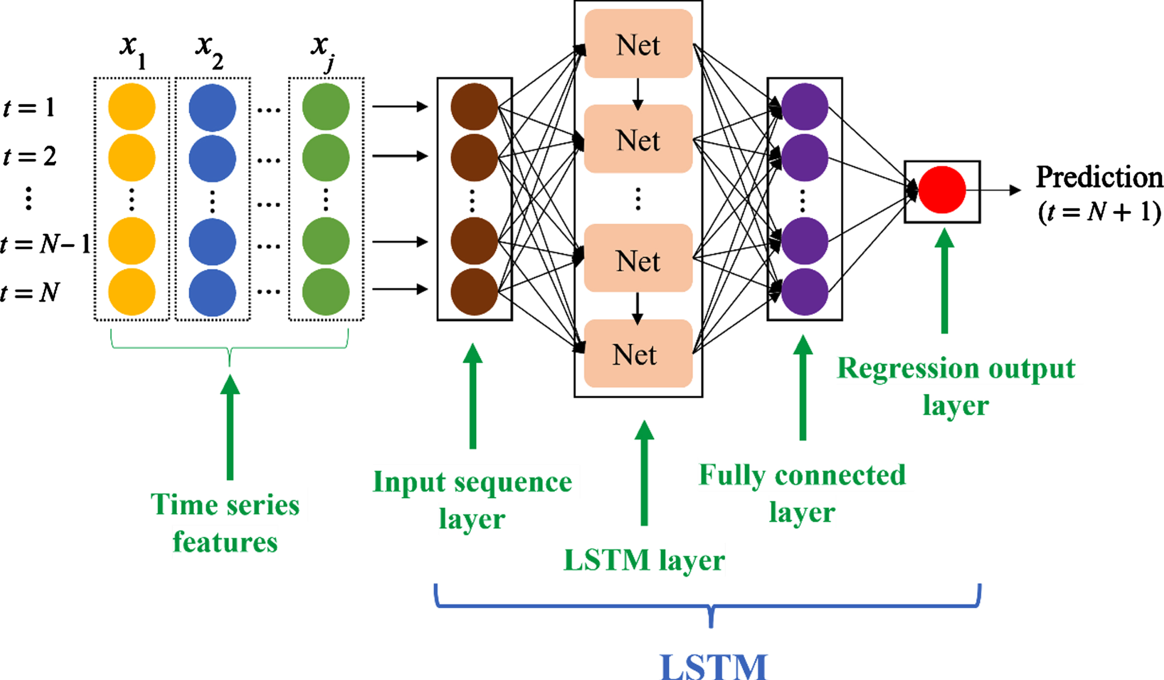
The multivariate numerical forecasting by an LSTM in deep learning, which is composed of an input sequence layer, LSTM layer, fully connected layer and regression output layer. A weather data of time series features is the input, where t is the time step, j is the amount of features, N is the observations of features and Net is a chunk of LSTM neural network. A forecast will be obtained by training the time series features in the LSTM.

4.2 Temperature forecasting results

The weather data are divided into 331 days for training data and 35 days for testing data. For the matrix, the rows represent time steps, and each column in the data constitutes a feature. Training data are to fit the model, and testing data are to validate the model by comparing its prediction with the raw data. When processing a time series problem with an LSTM in deep learning, the root mean square error (RMSE), the mean square error loss, and the mean absolute percentage error (MAPE) are often used as performance indicators. $RMSE = {(\frac{1}{N} \sum_{i = 1}^{N} {(y_{i} - {\hat{y}}_{i})}^{2})}^{1 / 2}$ (8) $Loss = \sum_{i = 1}^{N} {(y_{i} - \hat{y_{i}})}^{2} / N$ (9) $MAPE = \frac{1}{N} \sum_{i = 1}^{N} | (y_{i} - \hat{y_{i}}) / y_{i} |$ (10) where y_i is the real value, $\hat{y_{i}}$ is the forecast value, and N is the amount of y. The mean square error loss represents the difference between the real and forecast values which are extracted by squaring the average difference over the data. It is a measure of how close a fitted line is to the actual value. RMSE is the error rate by the square root of the mean square error loss. It is often used when assessing how well a model fits the data because it is measured in the same units as the forecast value. MAPE is a measure of forecasting accuracy and it is also commonly used in regression problems because of intuitive interpretation in terms of relative error. If the MAPE is lower than 10%, the forecast is highly accurate. If the MAPE is between 10% to 20%, the forecasting is good. If the MAPE is between 20% and 50%, the forecast is reasonable. If the MAPE is greater than 50%, the forecast is weak and inaccurate. For the above three indicators, the lower the value trained by the model, the higher the accuracy obtains for the forecast. Figure 3 indicates the training response for the weather data by a numerical dataset of 9 weather features (sea pressure, dew point temperature, relative humidity, wind speed, wind direction, sunshine rate, global solar radiation, visible mean and cloud amount) of every calendar day in 331 days is applied to train the LSTM for temperature forecasting. The contrast of training progress between the raw data and the preprocessed data is shown in Fig. 4. The lower the loss, the closer the fit is to the data. The results indicate that the preprocessed data are more able to converge than the raw data. In Table 1, the RMSE and MAPE of the forecast result by using preprocessed data are 2.8518 and 14.8993%, which are less than 4.0274 and 23.0538% by using the raw data. Figure 5 shows that the temperature forecast using the preprocessed data has a similar trend and higher resemblance between observed and forecast data. Therefore, the following works are all discussed with preprocessed data.

Fig. 3

The training response by a numerical dataset of 9 weather features (sea pressure, dew point temperature, relative humidity, wind speed, wind direction, sunshine rate, global solar radiation, visible mean and cloud amount) of every calendar day in 331 days is applied to train the LSTM for temperature forecasting.

Fig. 4

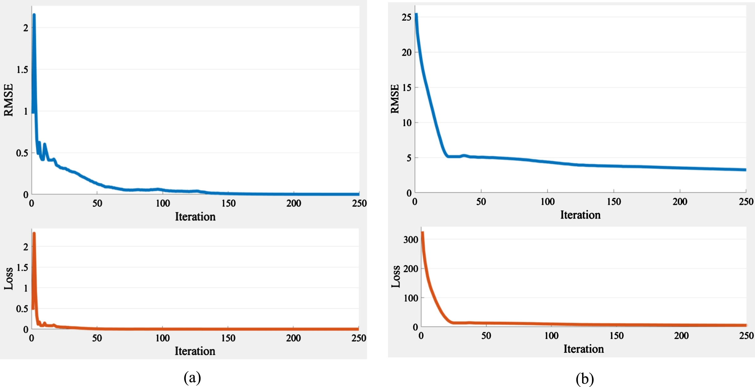
The training progress of the LSTM in deep learning using (a) preprocessed data and (b) raw data.

Table 1

The RMSE and MAPE of temperature forecasting by different predictor feature combinations

Data description	Predictor feature combinations	Deleted predictor feature	RMSE	MAPE(%)
Raw data	All	–	4.0274	23.0538
Preprocessed data	All	–	2.8518	14.8993
	SP+DP+GR+RH+WD+WS	SR, VM, CA	2.6400	12.2011
	DP+GR+RH+WD+WS	SP, SR, VM, CA	4.5456	24.0047
	SP+GR+RH+WD+WS	DP, SR, VM, CA	3.7247	18.6242
	SP+DP+RH+WD+WS	GR, SR, VM, CA	2.9600	14.0446
	SP+DP+GR+WD+WS	RH, SR, VM, CA	2.6838	11.7907
	SP+DP+GR+RH+WD	WS, SR, VM, CA	2.3043	5.5788
	SP+DP+GR+RH+WS	WD, SR, VM, CA	2.2389	5.1549
	SP+DP+GR+RH	WD, WS, SR, VM, CA	2.2215	5.0069
	SP+DP+GR	RH, WD, WS, SR, VM, CA	3.1068	14.5063
	SP+DP	GR, RH, WD, WS, SR, VM, CA	4.5809	23.0264

Fig. 5

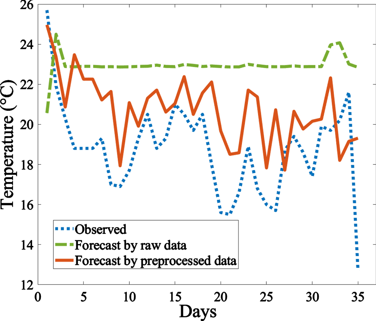
The forecast results of the raw data and the preprocessed data, and it shows that using the preprocessed data has a similar trend and higher resemblance with observed data.

The RMSE for using the remaining 9 features to predict the temperature is 2.8518, and the MAPE is 14.8993%. To obtain better results, multiple linear regression is used to select important predictor features in this work by describing the relationship between a dependent variable and one or more independent variables. The dependent variable y is also called the response feature and the independent variables x are also called predictor features. The multiple linear regression model used in this work is

$\begin{matrix} y_{i} = α_{0} + α_{1} x_{i 1} + α_{2} x_{i 2} + \dots \\ + α_{j} x_{ij} + ɛ_{i} i = 1, \dots, N \end{matrix}$ (11) where y_i is the i response, α_j is the j correlation coefficient, j is the amount of predictor features, x_ij is the i observation on the j predictor feature, ɛ_i is the i random error, and N is the scalar observations for each feature. In this work, temperature is the response feature y, and the remaining are the predictor features from x₁ to x₉. The result of temperature forecasting shown in Table 2 with the p-value between 0 and 1 representing the probability of obtaining the observed difference (or a larger one) in the outcome measure of the sample, since there are no differences between treatments in the data. The predictor feature of SR, VM and CA have ultimately testified as the least significant feature for predicting temperature, and the RMSE by using the remaining predictor features to predict temperature is decreased from 2.8518 to 2.6400.

Table 2

The p-value of the response feature temperature and predictor feature is calculated using the multiple linear regression

Predictor feature	p-value
Sea pressure	0.009
Dew point temperature	0.000
Relative humidity	0.000
Wind speed	0.005
Wind direction	0.009
Sunshine rate	0.230
Global solar radiation	0.000
Visibility	0.309
Cloud amount	0.248

To further analyze the correlation between the response feature and the predictor feature, Pearson’s correlation coefficient of two features (e.g., A and B) is a measure of their linear dependence and defined as $ρ (A, B) = \frac{1}{N - 1} \sum_{i = 1}^{N} (\frac{A_{i} - μ_{A}}{β_{A}}) (\frac{B_{i} - μ_{B}}{β_{B}})$ (12)

where μ_A and β_A are the mean and standard deviation of feature A, respectively, and μ_B and β_B are the mean and standard deviation of feature B. The Pearson’s correlation coefficient matrix of SP, DP, RH, WS, WD and GR is shown in Table 3. The result in Table 3 shows that from the highest intensity to the lowest, the SP, DP, GR, RH, WD and WS in order. Therefore, the above 6 predictor features are then deleted and the remaining predictor features are used to train the LSTM to verify the feature selection by multiple linear regression and Pearson’s correlation coefficient are reliable. The results are shown in Table 1. For the combination of features using five predictor characteristics, the larger RMSE and MAPE interpret the first characteristic of the deleted predictor characteristic column as more important, and the importance sequence is nearly the same as the result of Pearson’s correlation coefficient, besides WS and WD are opposite because of the minute difference. The results of using different combinations to train the LSTM are shown in Fig. 6(a), which indicates that it is not necessarily that the fewer the predictor features, the more accurate the predictions. The number of training features is based on different data types and the correlation between the predictor feature and response feature. There are two predictions in Fig. 6(b), which show the error of the temperature forecast value and the observed value, respectively. The best combination of this work for temperature forecasting is using SP, DP, GR and RH, which reaches the lowest RMSE 2.2215 and MAPE 5.0069%. Temperature is a feature that can be easily predicted in the atmosphere, and the results show that forecasting accuracy of temperature has increased by deleting the least effective features.

Table 3

Pearson’s correlation coefficient matrix shows the linear relationship between two features

Feature	SP	T	DP	RH	WS	WD	GR
SP	1.00	–0.88	–0.84	0.23	0.45	–0.43	–0.51
T	–0.88	1.00	0.87	–0.43	–0.32	0.36	0.69
DP	–0.84	0.87	1.00	0.07	–0.29	0.25	0.32
RH	0.23	–0.43	0.07	1.00	0.09	–0.23	–0.77
WS	0.45	–0.32	–0.29	0.09	1.00	–0.57	–0.17
WD	–0.43	0.36	0.25	–0.23	–0.57	1.00	0.32
GR	–0.51	0.69	0.32	–0.77	–0.17	0.32	1.00

Fig. 6

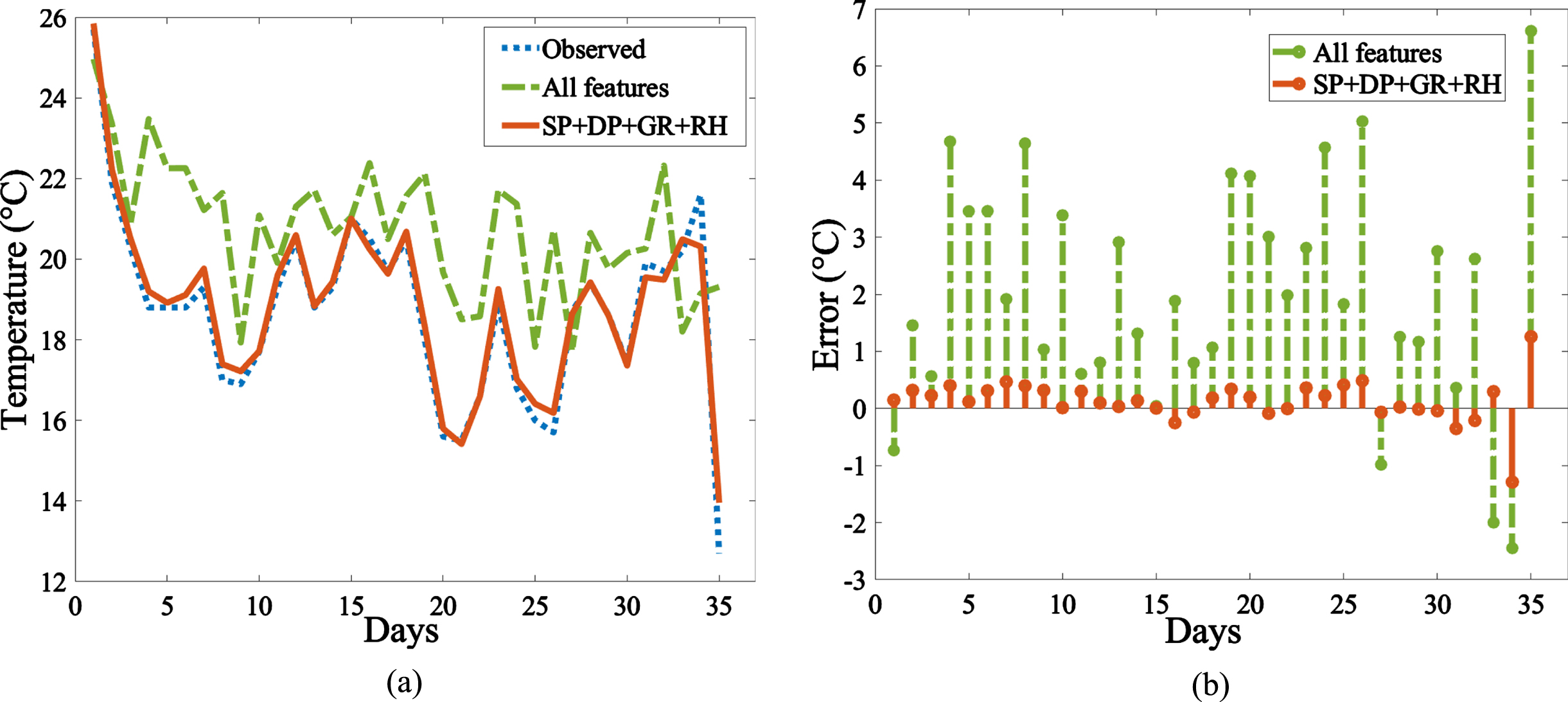
The temperature forecast using different combinations to train the LSTM model, where (a) shows the best combination is SP+DP+GR+RH and (b) shows that compared to the prediction by all features, it has the lowest error of RMSE 2.2215 and MAPE 5.0069%.

5 Conclusions

Conventionally, forecasters can only make subjective forecasts based on their experience in the absence of forecasting tools. Forecast quality is often limited by the forecaster’s understanding of regional characteristics and the influence of past experience. This study develops an LSTM by integrating multiple linear regression and Pearson’s correlation coefficients into feature selection to improve the temperature forecasting. The result shows that data preprocessing can improve training convergence and accuracy. In addition, using multiple linear regression and Pearson’s correlation coefficients as feature selection can improve forecasting accuracy by selecting important predictor features related to the response feature. Wind speed, wind direction, sunshine rate, visible mean, and cloud amount are the inert predictor features that must be deleted from the data, and sea pressure, dew point temperature, global solar radiation, and relative humidity are the remaining predictor features related to the temperature. The above four relational predictor features are used to train the LSTM, and the result shows that the forecasting error has a significantly decrease from RMSE 4.0274 to RMSE 2.2215 and MAPE 23.0538% to MAPE 5.0069%. This work has demonstrated that data standardization, multiple linear regression and Pearson’s correlation coefficients are reliable methods for data preprocessing in deep learning and selecting relational predictor features can increase the accuracy in the aviation weather forecasting.

Footnotes

Acknowledgments

This work was supported in part by the National Science and Technology Council, Taiwan, ROC under contract NSTC 111-2410-H-309-001-. The author is grateful to the reviewers and AE for their exceptional efforts in enhancing the style and clarity of this paper.

Data availability

The input weather information is collected from the database: .

Declaration of interest statement

The authors declared that they have no conflicts of interest in this work.

References

Richardson

L.F.

, Weather prediction by numerical process. Cambridge University Press, UK, 2010.

Carrassi

, Bocquet

, Bertino

and Evensen

, Data assimilation in the geosciences: An overview of methods, issues, and perspectives, Wiley Interdisciplinary Reviews-Climate Change 9(5) (2018), 1–50.

Vlachas

P.R.

, Pathak

, Hunt

B.R.

, Sapsis

T.P.

, Girvan

, Ott

and Koumoutsakos

, Backpropagation algorithms and reservoir computing in recurrent neural networks for the forecasting of complex spatiotemporal dynamics, Neural Networks 126 (2020), 191–217.

Bocquet

, Brajard

, Carrassi

and Bertino

, Bayesian inference of chaotic dynamics by merging data assimilation, machine learning and expectation-maximization, Foundations of Data Science 2(1) (2020), 55–80.

Geer

A.J.

, Learning earth system models from observations: Machine learning or data assimilation, Philosophical Transactions of the Royal Society A: Mathematical Physical and Engineering Sciences 379(2194) (2021).

Kashinath

, Mustafa

, Albert

, Wu

, Jiang

, Esmaeilzadeh

, Azizzadenesheli

, Wang

, Chattopadyay

, Singh

, Manepalli

, Chirila

, Yu

, Walters

, White

, Xiao

, Tchelepi

H.A.

, Marcus

, Anandkumar

and Hassanzadeh

, Physics-informed machine learning: Case studies for weather and climate modelling, Philosophical Transactions of the Royal Society A: Mathematical Physical and Engineering Sciences 379(2194) (2021).

Sangiorgio

and Dercole

, Robustness of LSTM neural networks for multi-Step forecasting of chaotic time series, Chaos, Solitons and Fractals 139 (2020).

Hong

S.J.

, Kim

J.H.

, Choi

D.S.

and Baek

K.H.

, Development of surface weather for east model by using LSTM machine learning method, Korean Meteorological Society 31(1) (2021), 73–83.

, Du

, Wang

, Jiang

and Ren

, Satellite image prediction relying on GAN and LSTM neural networks. IEEE International Conference on Communications, 2019, pp. 1–6.

10.

Zhu

, Zhu

, Han

and Wang

, The application of deep learning in airport visibility forecast. Atmospheric and Climate Sciences 7(3) (2017), 314–322.

11.

Zhang

, Wu

, Chen

, Zhang

, Xie

, Huang

and He

, Weather visibility prediction based on multimodal fusion, IEEE Access 7 (2019), 74776–74786.

12.

Deng

, Cheng

, Han

and Lin

H.X.

, Visibility forecast for airport operations by LSTM neural network, International Conference on Agents and Artificial Intelligence, 2019, pp. 466–473.

13.

Meng

, Qi

, Zuo

, Chen

, Yuan

and Xiao

, Multi-step LSTM prediction model for visibility prediction, International Joint Conference on Neural Networks, 2020, pp. 1–8.

14.

Salman

A.G.

, Heryadi

, Abdurahman

and Suparta

, Single layer & multi-layer long short-term Memory (LSTM) model with intermediate variables for weather forecasting, Procedia Computer Science 135 (2018), 89–98.

15.

Vlachas

P.R.

, Byeon

, Wan

Z.Y.

, Sapsis

T.P.

and Koumoutsakos

, Data-driven forecasting of high-dimensional chaotic systems with long short-term memory networks, Proceedings of the Royal Society A: Mathematical Physical and Engineering Sciences 474(2213) (2018).

16.

Elsaraiti

and Merabet

, Application of long-short-term-memory recurrent neural networks to forecast wind speed, Applied Sciences 11(5) (2021), 2387.

17.

, Ye

, Pei

, Lu

, Dai

, Li

and Wang

, A combined model for short-term wind power forecasting based on the analysis of numerical weather prediction data, Energy Reports 8 (2022), 929–939.

18.

Bengio

, Simard

and Frasconi

, Learning long-term dependencies with gradient descent is difficult, IEEE Transactions on Neural Networks 5(2) (1994), 157–166.

19.

, Wang

S.L.

and Xie

D.B.

, Research on radar clutter recognition method based on LSTM, The Institution of Engineering and Technology 19 (2019), 6247–6251.

20.

Wasserstein

R.L.

and Lazar

N.A.

, The ASA statement on p-values: Context, Process, and Purpose, The American Statistician 70(2) (2016), 129–133.

21.

Pan

, You

, Liu

and Zhang

, Pearson correlation coefficient-based pheromone refactoring mechanism for multi-colony ant colony optimization, Applied Intelligence 51 (2021), 752–774. https://doi.org/10.1007/s10489-020-01841-x

22.

Edelmann

, Mori

T.F.

and Szekely

G.J.

, On relationships between the Pearson and the distance correlation coefficients, Statistics and Probability Letters 169(108960) (2021).

23.

Lihua

, Simulation physics-informed deep neural network by adaptive Adam optimization method to perform a comparative study of the system, Engineering with Computers 38 (2022), 1111–1130. https://doi.org/10.1007/s00366-021-01301-1

24.

Salem

, Kabeel

A.E.

, El-Said

E.M.S.

and Elzeki

O.M.

, Predictive modelling for solar power-driven hybrid desalination system using artificial neural network regression with Adam optimization, Desalination 522(115411) (2022).