A comprehensive review on the development of copulas in financial field

Abstract

The Copula concept has long been used in many applications, especially in the financial field. This concept was first used in 1959 by Sklar in his mathematical work and greatly assisted in the applications of financial and insurance areas. The copula functions have been widely used in dependence modeling. In this study, we look at how the copula began to develop from a basic form to a more advanced form through studies that previous researchers have made. Throughout this study, we find various types of the copula, and each exhibits its own characteristics lying under two main families, Elliptical and Archimedean copulas. Our findings suggest that copula is vital in solving problems in statistical dependence measures and joint marginal distribution functions. This comprehensive study served as a review paper on the development of copulas from their initial existence to their latest evolution.

Keywords

Copula financial field decision-making insurance marginal distribution

1 Introduction

The financial field involves managing money and how an individual, company, or government agency acquires and spends money. This leads to financial services that allow consumers and businesses to acquire financial goods from money management. For instance, a payment system provider is a financial service when it accepts and transfers funds between payers and recipients. The financial services sector is one of the most critical segments of the economy. It helps drive a nation’s economy, providing the free flow of capital and liquidity in the marketplace.Financial modeling is the process of creating a model of a scenario in which a financial choice must be made. Financial modeling is being utilized by an increasing number of businesses these days for purposes such as risk assessment, strategy planning, and review of capital budgeting since it offers numerous benefits to both managers and end users. Therefore, financial modeling is a crucial process in the finance industry. However, the recent recession has necessitated a re-evaluation of modeling in the financial services industry [50]. Moreover, aggregating individual risks is one of the most pressing problems in risk management. For example, assume the random variables modeling individual risks are either independent or dependent on a common factor that allows the reduction of independent variables case. This can be done by eventually adding one new variable (describing the common factor) to the set of risks, effectively solving or at least discarding the problem. The task becomes considerably more complicated when modeling fully dependent random variables or when one does not know the exact joint distribution to construct a huge dependency set between the provided individual risks.

Prior to the above problem, a common approach is to assume that the vector of risks has Gaussian behavior (with some specific covariance matrix), but this is unlikely to be the case since not all threats are normally distributed. Consider the extremely asymmetric loss distribution of a pool of credit, or the normal joint distribution may fail to capture some important unique elements of the dependency of the examined risks, such as tail dependence. In addition, we emphasize that we frequently lack as much information about the joint distribution as we do about each individual risk [49]. Therefore, the idea of a copula that provides a robust and approachable framework for describing risks is introduced. Copula also provides a robust and user-friendly mechanism for risk analysis in risk management. Copula is derived from the Latin noun copula, meaning ”link, tie, bond,” and refers to uniting two things. This word was first used in 1959 in Abe Sklar’s mathematical work [81], but it has recently gained favor in financial applications. A copula is a multivariate distribution function that joins or links univariate marginal distribution functions. A distribution function distributes probabilities as a function of outcomes; that is, the distribution function offers the probability for each outcome [8].

In the 1950s, the idea of a copula was first established, with its discovery linked to the works of [28, 31, 81]. Fréchet first introduced a distribution with a specified marginal [31]. For random variables Y₁ and Y₂ specified on [0, 1] probability space, he worked on a problem involving the bivariate distribution functions F₁ (y₁) and F₂ (y₂). The distribution function F (y₁, y₂) = F (y₁) F (y₂) is a member of the set F (F₁, F₂), which Fréchet [31] noted is not empty even if the random variables are independent. Many researchers have been motivated to work on this issue, including his own pupils Féron [28] and Sklar [81]. Then, Féron [28] constructed some functions on the unit cube [0, 1] that coupled three-dimensional distributions with their one-dimensional marginal distributions. Connecting d-dimensional distributions with corresponding one-dimensional marginal distributions, Sklar [81] constructed such functions on the unit d-cube for any d > 2 in 1959. In addition, Sklar [81] worked on the fundamental features of these functions and shared his findings with Fréchet [31]. Fréchet [31] posed the task of identifying the link between d-dimensional cumulative distribution functions and their marginal one-dimensional cumulative distribution functions. Sklar responds to this query by introducing the copula idea that bears his name, Sklar’s theorem. As defined by Sklar, Copula is a statistical function that connects n-dimensional distributions to their one-dimensional margins. In the 1960s, the notion of copulas did not evolve. The study published by Sklar in 1959 [81] lacked proof of Sklar’s theorem. Therefore, some authors rediscover copula [51, 85]. They demonstrate Sklar’s theorem without referring to the copula by its proper name. In their publication, [76] provide an innovative proof to copulas for two-dimensional distribution, and they formulate their proof as Lemma 5. Most of the results on copulas acquired until 1980 were obtained in conjunction with problems that arose from investigating probabilistic metric spaces [77]. The academic work that [75] is the first one to link the concept of a copula to the investigation of the relationship between random variables. The field of statistics discovered copula shortly after the publication of this study.

In this regard, our focus shifted to the interplay between random variables. Since the behavior of a univariate marginal distribution function can be determined, we can use multivariate distributions to learn more about marginal distributions’ interaction or gain a more thorough understanding of their dependencies. We will look at why copulas are replacing linear correlation as the go-to tool for solving financial problems because they are much more accurate and popular. The financial industry is well-known for misusing techniques. Correlation has been labeled a "minefield for the unwary" due to the frequency with which it is inappropriately applied to problems. Because correlation is not a universal dependency measure in risk management, this will not work. For instance, if we want to represent the relationship or reliance between two risky variables X and Y, we will likely employ linear correlation. When our random variables follow a multivariate normal distribution, a correlation of +1 tells us that the two variables are positively dependent (rises or falls together), a correlation of -1 tells us that they are negatively dependent (one rises and the other falls), and a correlation of 0 tells us that the two variables are independent. Furthermore, correlation is restricted in a normal or elliptical universe since it cannot model asymmetries. Regarding financing, there is a much stronger relationship between significant losses than between significant gains. The correlation cannot be assumed invariant by any modifications of the variables it is based on. For example, the correlation between variable X and variable Y is not the same as that between log(X) and log(Y). As a result, the transformations we apply to our data can affect the correlation estimations we obtained [64]. In light of these limitations, copula, introduced at the outset as an alternative to correlation as a measure of reliance, becomes more appealing. Unlike correlation, copulas benefit from invariance under strictly increasing random variable transformations. Copula is superior to correlation since it remains unchanged when the units of measurement are changed, for as, when going from X to log(X). Rather than using a single statistic, like correlation, to summarise the dependence structure, we can utilise a model for the dependence structure that reflects our in-depth understanding of the risk management challenge at hand. In order to establish marginal models for individual risk factors and copula models for their dependence structure, we can use the copula as a multivariate distribution function.

A copula can be used to suggest an appropriate form for the joint distribution if the marginal distributions are known. For this purpose, we have access to numerous copula families from which to choose. This allows us to select a specific copula family based on the random variables of the multivariate data we are attempting to model. This means we can generate multivariate distribution functions by combining arbitrary marginal distributions and extracting copulas from well-known multivariate distribution functions. Knowing the right copula to use when modeling random variables will help determine the right dependence structure. Since each copula has a totally different dependence structure, it is necessary to choose a copula that describes the true dependence structure as well as possible [64]. Derived from distribution functions, more advanced copulas allow us to select the most appropriate model for a given problem from various parametric families. Elliptical copulas and Archimedean copulas are the two main kinds of copulas [23]. These families share a standard structure in their two arguments, making them a valuable part of both bivariate and multivariate copulas. Implicit copulas, which belong to the class of Elliptical copulas, are frequently used as a standard. However, Elliptical copulas can only have radial asymmetry; thus, they have no closed-form expression. It makes sense that in many financial applications, the correlation between extremely large losses would be higher than between extremely large earnings. This kind of asymmetry cannot be modeled using Elliptical copulas. Gaussian copula and Student-t copula are examples of Elliptical copulas. In the study conducted by [79], they recommended using a copula regression to analyse multivariate, longitudinal claims data to account for the unique features of insurance premiums at the policy level. To analyse the semi-continuous claim costs for each coverage type, the model employs the Tweedie double generalised linear model and a Gaussian copula to account for cross-sectional and temporal dependence among the multilevel claims. Then, the second kind of copula is Archimedean copulas. These copulas are also known as explicit copulas and are widely used thanks to their simplicity of construction. This class has many copula families, many of which share desirable qualities. Due to their attractive features and relatively straightforward construction, they use extensively in financial and insurance-related applications [25]. Example of Archimedean copulas is Clayton, Gumbel, and Frank copulas. Genest and Mackay’s [34] study demonstrated that Archimedean copulas could have only a single component in certain circumstances regarding Kendall’s measure of association. However, we will go through many other developments on copula in this study and their unique characteristics.

Motivated by the literature gap discussed above, this paper intends to deepen understanding of copulas’ role in solving a finance-related problem. Many queries will arise when we explore the theory of copulas; for example, why are copulas significant for research and analysis in this financial field? To answer this question, there are two significant reasons for this study. First, it may be used to learn statistical dependence measures with its application in finance, and second, it can be used to create different types of joint distributions. To establish joint distributions, we can use copula to couple marginal distributions of data used in research. The beauty of copula is that it allows us to extract the dependence structure from marginal distributions jointly. It is useful when studying many variables as it is a multivariate dependence structure [12].

This research makes the following key contributions. First, this research can serve as a valuable, comprehensive review for those who intend to gain more knowledge and information on copula, especially regarding the applications in finance. Second, there needs to be more research made on this topic. We noticed that most of the review papers only focused on the copula itself and not on the applications in the financial field. So, this paper also contributes as a guideline to other researchers in assisting their understanding of copula in the financial field.

The remaining of this paper is presented in 6 sections. In the upcoming section, the theory of copula is presented. Then, we will go through the families of the copula in the third section, the elliptical and Archimedean copulas. After that, in the fourth section, a shift from general copula to pair copula construction which is the PCC, is discussed. Furthermore, more information about PCC is presented in the fifth section, and a discussion is made in the sixth section. Lastly, we presented an overall conclusion of this study in the seventh section.

2 Theory of copulas

This section will explain the theory that is related to copulas. First, we will look through Sklar’s theorem. Then we will proceed to the following theory, a d-dimensional copula followed by Fréchet-Hoeffding bound inequality and the independent copula.

2.1 Sklar’s theorem

Sklar’s theorem makes copulas crucial [81]. Any multivariate joint distribution can be described by its marginal distribution, according to this theorem. Let J be d-dimensional distribution function with marginals F₁, F₂, …, F_d. Then, there exists d-copula C^d such that, J (x₁, x₂, …, x_d) = C^d (F₁ (x₁) , F₂ (x₂) … F_d (x_d)) for all x ∈ R^d. The copula is uniquely determined, if F₁, F₂, …, F_d are continuous. Otherwise, C^d is uniquely determined on (range of F₁), x (range of F₂), x … x (range of F_d). Contrarily, if C^d is a d-copula, and F₁, F₂, …, F_d are distribution functions, then the function J in (1) is d-dimensional cdf with marginals F₁, F₂, …, F_d [11].

2.2 A d-dimensional copula

A d-dimensional copula is a function “C” from I^d = [0, 1] ^d to I = [0, 1] if and only if it satisfies the following conditions:

For every m in I^d, C (m₁, m₂, dotsi, m_d) =0 if at least one of m is equal to zero.

If all m’s are set to one then for every k ∈ 1, 2, dotsi, d, C (m) = m_k.

C is d-increasing, for all (a₁, …, a_d), (b₁, …, b_d) in I^d such that a_i ≤ b_i, V_c ([a, b]) ≥0, $\begin{matrix} \sum_{i_{1} = 1}^{2} \sum_{i_{2} = 1}^{2} . . . \sum_{i_{3} = 1}^{2} & (- 1)^{i_{1} + i_{2} + . . . + i_{k}} \\ C (m_{1_{i_{1}}}, m_{2_{i_{2}}}, . . ., m_{d_{i_{d}}}) \geq 0 \end{matrix}$ All above properties of d-copula is a multivariate version of the bivariate copula. Condition (1) defines the grounded property, condition (2) defines copula margin if (d - 1) variables are known, and condition (3) defines C volume of rectangle [a × b] for any d-dimension. Furthermore, any convex linear combination of copulas is a copula, i.e., $\sum_{i_{1}}^{d} a_{i} C_{1}$ for all a_i > 0 and ∑a_i = 1 [11].

2.3 Fréchet-Hoeffding bound inequality

Fréchet-Hoeffding theorem establishes the minimal and maximal bounds on the set of copulas. For every d-copula, the Fréchet-Hoeffding bound inequality is given by: $C_{L}^{d} \leq C (m_{1}, m_{2}, . . ., m_{d}) \geq C_{U}^{d}$ and m ∈ [0, 1] ^d where, $C_{L}^{d}$ and $C_{U}^{d}$ and defined as $max (\sum_{i_{1}}^{d} m_{i} - d + 1, 0)$ and min(m₁, m₂, …, m_d) respectively. Notice that, for d > 2, the lower bound $C_{L}^{d}$ is not a copula [11].

2.4 Independence copula

The independence copula is the copula that results from a dependency structure in which each individual variable is independent of the other. If the random variables are independent, then copula density is equal to the product of the marginal distribution of the random variables. Let all m in the unit interval, and then the copula is independent if and only if, C^d (m) = m₁, m₂, . . . , m_d. For all d ≥ 2, the continuous random variables X₁, X₂, …, X_d are independent if and only if their d-copula is C^d (m).

3 Copula families

Elliptical and Archimedean copulas are the two types of copulas that exist. We are interested in bivariate one-parameter copula families that are continuous, interpolate between independence and the Fréchet upper bound, and support all of (0, 1) ². These families are symmetric in both arguments and can be utilised for both bivariate and multivariate copulas [65].

3.1 Elliptical copulas

Copulas having elliptical distributions are known as elliptical copulas. The t-student, logistic, and Gaussian (normal) distributions are all examples of distributions. Implicit copulas are a class of elliptical copulas commonly used as a benchmark model. Elliptical copulas have the disadvantage of not having closed-form expressions and being limited to radial asymmetry. With elliptical copulas, such asymmetries are impossible to simulate. It appears reasonable to anticipate that significant losses are more correlated than large gains in many insurance and financial applications. The upper and lower tail dependence factors are equal because elliptical distributions are radially symmetric. They are simply the distribution functions of component-wise converted elliptically distributed random vectors [64].

A normal (Gaussian) copula is an example of an Elliptical copula. The Gaussian copula is the most popular for modeling the association in finance and insurance risk problems [26]. It is the multivariate normal distribution’s copula. The copula of n-variate normal distribution is, $C_{ρ}^{Gauss} U = Φ_{ρ}^{n} (φ^{- 1} (u_{1}) . . . φ^{- 1} (u_{n}))$ where Φ_ρ - standard multivariate normal distribution function with matrix ρ and ρ^-1 the inverse of the standard univariate normal distribution function.

Gaussian copulas have no upper or lower tail dependence, and they are the most commonly employed in finance since they are the copula of a log-normal vector. It conveys dependence in the same way as a multivariate normal distribution does, but for variables with arbitrary marginals. If n = 2, by expression above we have $C_{ρ}^{Gauss} (u, v) = Φ_{ρ}^{2} (φ^{- 1} (u) . . . φ^{- 1} (v))$

Fig. 1

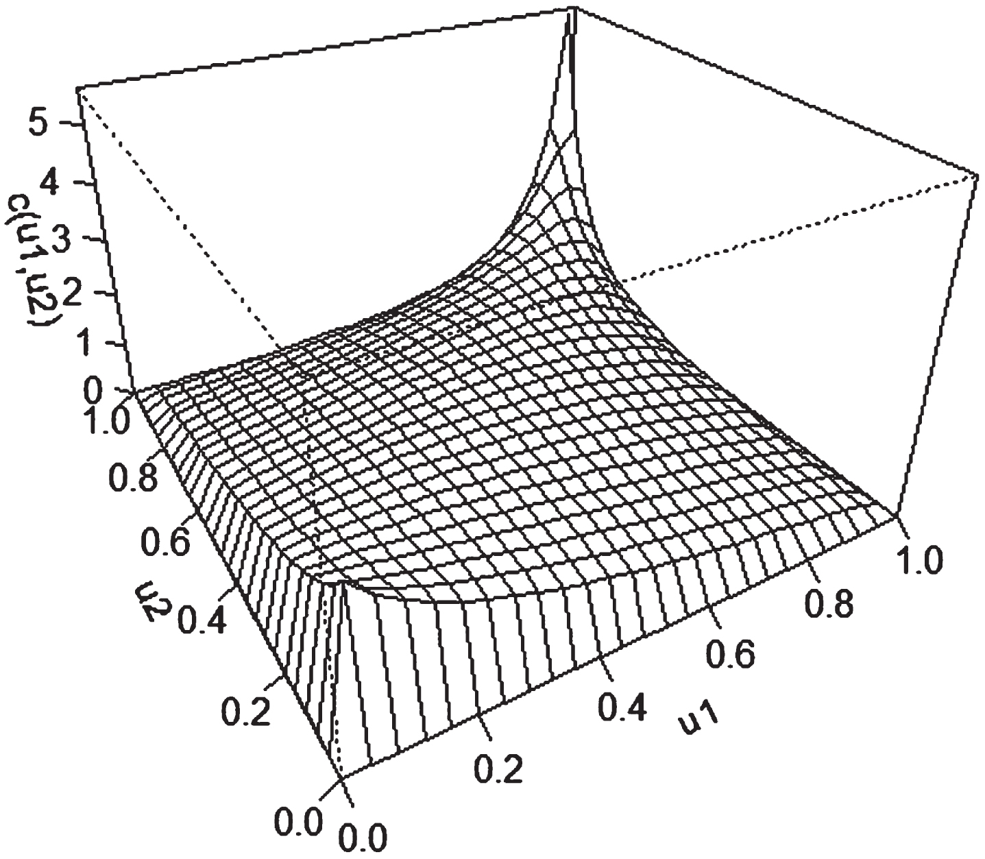
Gaussian copula density.

Another example of an Elliptical copula is the Student-t copula. It is a copula of the multivariate Student-t distribution. Let X be a vector with n variate Student-t distribution with v degrees of freedom, mean vector μ (of μ > 1) and covariance matrix v/(v - 2) ∑, for v > 2 since if v ≤ 2, the covariance matrix is not defined. Then X can be represented as $X = μ + \frac{\sqrt{v}}{\sqrt{S}} Z,$ where Z ∼ N_ρ (0, ∑) and independent S, which is $X_{v}^{2}$ and the density function of the multivariate t-distribution with v degrees of freedom is $f (x) = \frac{Γ [\frac{(v + p)}{2}]}{(π v)^{\frac{P}{2}} Γ (\frac{v}{2})} | \sum^{- \frac{1}{2}} [1 + v^{- 1} (x - μ)^{T} \sum^{- 1} (x - μ)]^{- \frac{v + p}{2}}$ For a bivariate case, Student-t has the following form, $\begin{matrix} C_{v, p}^{t} (u, v) & = \int_{- \infty}^{t_{v}^{- 1}} \int_{- \infty}^{t_{v}^{- 1}} \frac{1}{2 π \sqrt{(1 - ρ^{2})}} \\ {{1 + \frac{s^{2} - 2 ρ st + t^{2}}{v (1 - ρ^{2})}}^{- \frac{(v + 2)}{2}}} dsdt \end{matrix}$ The Student-t copula has upper tail dependence, unlike the Gaussian copula.

Fig. 2

Student-t copula density.

3.2 Archimedean copulas

Archimedean copulas, also known as explicit copulas, have a wide range of applications due to their ease of construction. Members of this class have a wide range of desirable characteristics, and they belong to a large number of copula families. Because of their simple shape and pleasant qualities are often utilised in financial and insurance applications [64].

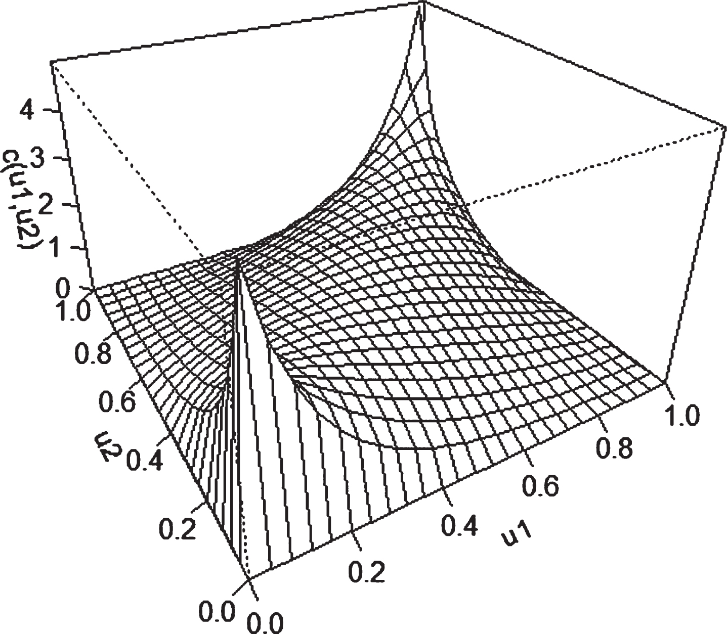
There are various examples of Archimedean copula. One example is Clayton copula. It is an asymmetric Archimedean copula in which the negative tail is more dependent than the positive tail. This copula is given by: letting X and Y be random variables with joint distribution functions. Then the Clayton copula is, $C_{θ}^{Clayton} (u, v) = \max ((u^{- θ} + v^{- θ} - 1)^{\frac{- 1}{θ}})$ Another example of an Archimedean copula is the Gumbel Hougard copula. Let X and Y be random variables with a joint distribution function. A bivariate extreme value distribution is given by $H_{θ} (x, y) = \exp (- (e^{- θ x} + e^{- θ y})^{\frac{1}{θ}})$ . For all x, y in $ℝ$ , where θ ≥ 1. Take note that a bivariate copula C is an extreme value copula if C (u^t, v^t) = C^t (u, v) for all t > 0.Then the copula of X and Y, which is a one-parameter family of copulas known as Gumbel Hougaard is $C_{θ}^{Gumbel} (u, v) = \exp (- [(- ln u)^{θ} + (- ln v)^{θ}]^{\frac{1}{θ}})$ . Parameter θ may take values in the interval [1, inf), and it also controls the degree of independence between u and v [64]. Then one of the famous Archimedean copula widely used is the Frank copula. Let X and Y be random variables with a joint distribution function. Then the Frank copula is $C_{θ}^{Frank} (u, v) = - \frac{1}{θ} ln (1 + \frac{(e^{- θ u} - 1) (e^{- θ v} - 1)}{e^{- θ} - 1})$

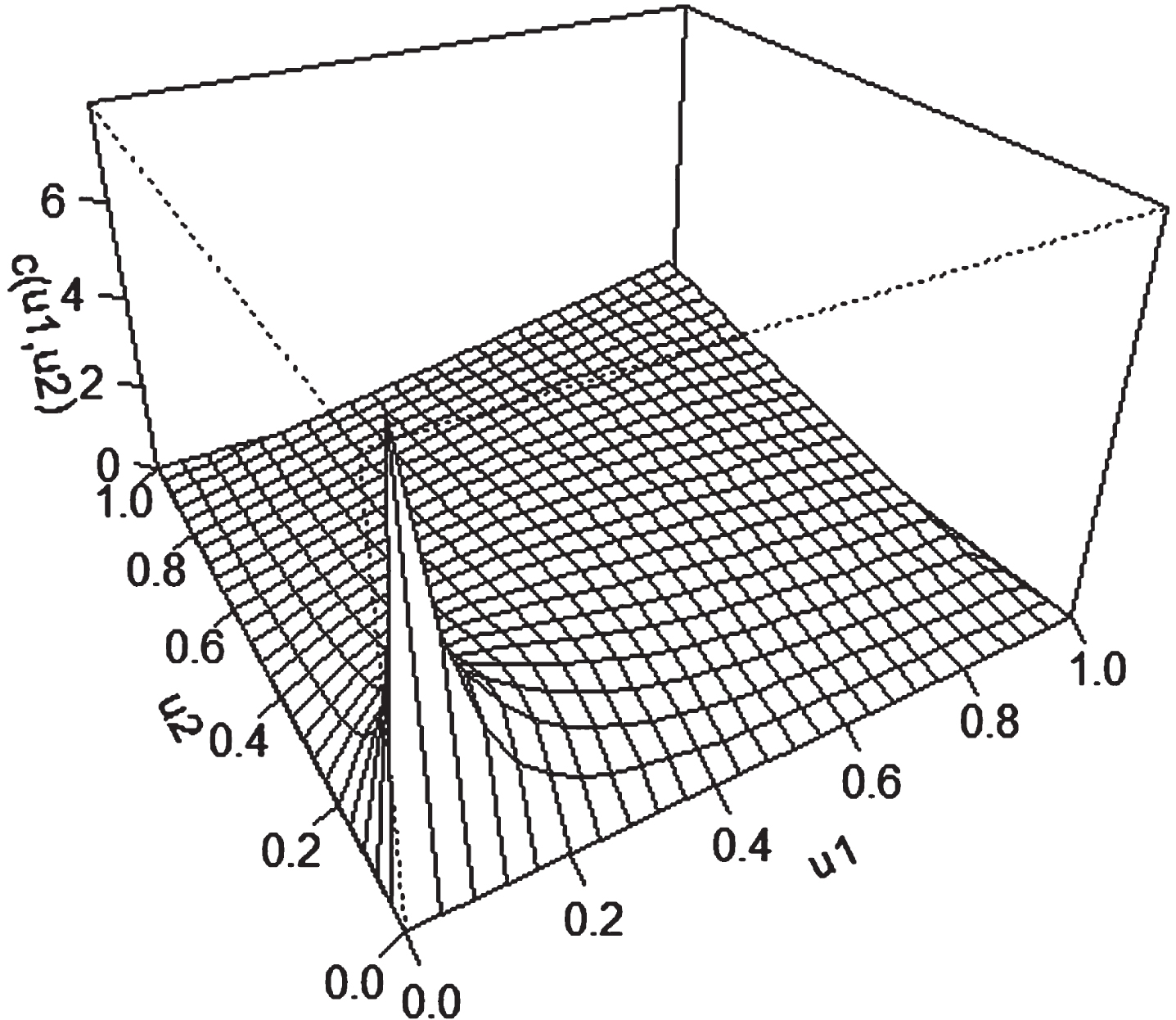
The Frank copula is symmetric, which means the dependence between positive and negative returns is correlated. The parameter θ ∈ (- ∞ , ∞) ∖ {0} controls the degree of dependence between u and v [64].

Fig. 3

Clayton copula density.

Fig. 4

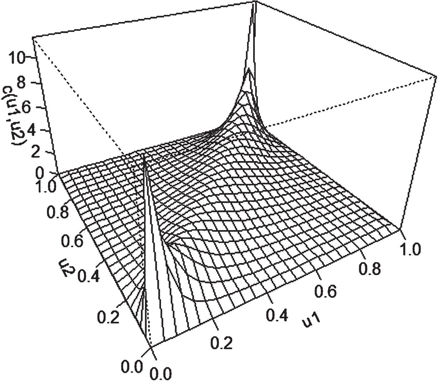
Gumbel copula density.

Fig. 5

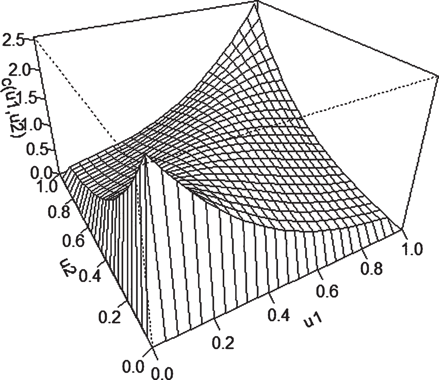
Frank copula density.

4 A shift to pair copula constructions (PCC)

Statistical researchers have been given various new prospects due to exceptional technical advancements in recent decades. The increasing availability of massive data sets and the emergence of enormous databases have necessitated the development of multivariate analysis methodologies. Many of them are based on the assumption of a multivariate parametric distribution. The multivariate normal distribution has been the most popular due to its numerous appealing qualities. Though it has numerous natural applications, it cannot account for heavy tails, skewness, nonlinear dependence, or severe joint events. As a result, varieties of alternatives, including multivariate extensions of well-known univariate distributions, have been offered.

4.1 The justifications of shifting

Due to its advantages, we know that the multivariate normal distribution is the most popular multivariate analysis method researchers widely use. Even though they are a helpful method, they also have the bad trait that their flexibility reduces as the dimension increases, limiting the spectrum of dependence they may portray. Furthermore, their univariate marginal distributions are all of the same types and have a similar shape. In the multivariate t-student distribution, for example, each variable has its own location and scale parameters, and each pair has its correlation. However, all share the degrees of freedom parameter, which affects the frequently essential tails. One way to deal with these issues is to change the original variables into a more tractable mathematical distribution. Using the cumulative distribution function (cdf) for each variable [41].

For bivariate models (d = 2), there exists a long and varied list of copula families [41]. As soon as d ≥ 3, the catalog of available copula is significantly reduced [36]. Several well-known Archimedean copulae generalize to higher dimensions [56]. However, they are exchangeable. As a result, all pairwise dependencies are the same, making them unsuitable for data with more diverse dependency patterns. Furthermore, as d increases, the constraints on their parameters, and hence the spectrum of dependency they can represent, become increasingly severe. An Elliptical copula, most likely the Gaussian or t-student, is another common option in higher dimensions. When pairwise dependencies are fairly symmetric and, more critically, extremes do not appear to occur simultaneously, the former may be a good alternative. The t-student copula is desirable if the data appear to be tail dependent. Although each pair of variables correlates, the degrees of freedom parameter is shared. The Student-t, like the multivariate Archimedean copula, is best suited when the tail behavior of all pairings is comparable [41]. Therefore, a flexible and more versatile method is introduced by [46], which is the pair copula constructions (PCC).

5 Pair copula constructions (PCC)

The growing availability of multidimensional data for complex systems has rekindled interest in multivariate modeling, particularly copula. As a result, there is now a broad and diverse list of the parametric bivariate copula, all fully suitable for bivariate models. In larger dimensions, however, the choice of parametric copula is still limited [36]. Recent research has tended to favor hierarchical, copula-based systems. The pair copula (PCC) architecture is perhaps their most promising. Initially proposed by [46], it has been further explored and discussed by [5, 15] and in an inferential context by [3]. Recently, there have been many papers on PCC in the literature, particularly in financial applications. Bayesian inference on PCC is the topic of [59], while [48] explores tail dependence in such constructions. [83] present a non-parametric petroleum-related application of PCC. The combination of its basic construction and high adaptability is likely the reason for the PCC’s rising popularity. They can model various complicated dependencies despite being created entirely from pair copula. PCC often minimizes dimension by pairing the variable set and creating a versatile dependency structure. Regarding the number of copula functions that could be used in the construction, PCC is more versatile [24]. D-Vine (drawable vine copula), C-Vine (canonical vine copula), and R-Vine (regular vine copula) are the three structures that make up the PCC system.

5.1 The PCC

In this section, we will look further into the PCC, the pair copula construction, to study their usage and advantages. Recent improvements in high-dimensional copula models have favored hierarchical structures based on the pair copula construction model (PCC), commonly known as vine copulas. It is a revolutionary new approach to building complex multivariate highly dependent models similar to traditional hierarchical modeling. The PCC’s growing popularity is likely due to its simple structure and high adaptability. Despite being constructed entirely of pair copula, they can model many complex dependencies [42]. The decomposition of a multivariate density into a cascade of pair copula is used to model the original variables and their conditional and unconditional distribution functions [3]. The following is a representation of an n-dimensional vine:

(n - 1) trees (T);

The tree j has (n - 1 + j) nodes and (n - j) edges;

Each edge corresponds to a bivariate copula density;

The borders of the tree j become nodes of the tree j + 1;

Complete decomposition is defined by n (n - 1)/2 edges and marginal densities of each variable, that is, n (n - 1)/2 bivariate copula densities and N marginal.

Using pair-copula constructions, the joint copula density c can be expressed as a product of several bivariate pair-copulas. Let f be the joint density function of n random variables X = (X₁, …, X_n),

\begin{matrix} f (X_{1}, . . ., X_{n}) = & f (X_{n} \cdot f (X_{(n - 1)} | X_{n}) \cdot \\ f (X_{(n - 2)} | X_{(n - 1)}, X_{n}) \cdot \end{matrix}

(1)

f (X_{1} | X_{1}, . . ., X_{n})

The conditional density is denoted by f (. | .) [3]. Despite this, the PCC has a few flaws. A broad multivariate model can be deconstructed precisely using pair-copula and conditional cumulative distribution functions (cdfs) as arguments in a hierarchical structure, for example,

$c_{12 | 3} (F_{1 | 3} (x_{1} | x_{3}) . F_{2 | 3} (x_{2} | x_{3}); x_{3})$ (2) where the c_ij|k is the copula corresponding to the conditional cdf F_ij|k of X_i, X_j and X_k and F_i|k the cdf of X_i given X_k. However, in order for inference to be rapid, flexible, and robust, this pair-copula must be assumed to be independent of the conditioning variables, except through conditional distributions,

$c_{12 | 3} (F_{1 | 3} (x_{1} | x_{3}), F_{2 | 3} (x_{2} | x_{3}))$ (3) Hence, although the general pair-copula decomposition (2) can represent all continuous multivariate distributions with strictly increasing marginal distributions, realistically, one must resort to the simplified version (2) [42]. So, here are the simplified PCC. Consider three random variables x₁, x₂, x₃ having the joint cdf F₁₂₃ (x₁, x₂, x₃). Assuming that F₁₂₃ (x₁, x₂, x₃) is absolutely continuous with strictly increasing marginal distributions F₁ (x₁) , F₂ (x₂) and F₃ (x₃), the corresponding probability density function (pdf) f₁₂₃ (x₁, x₂, x₃) is factorised as

$\begin{matrix} f_{123} (x_{1}, x_{2}, x_{3}) = & f_{3} (x_{3}) f_{2 | 3} (x_{2} | x_{3}) \\ f_{1 | 23} (x_{1} | x_{2}, x_{3}) \end{matrix}$ (4) One rewrites (3) in terms of copula densities to obtain a PCC. Let c₂₃ (F₂ (x₂) , F₃ (x₃)) be the density of the copula c₂₃ (F₂ (x₂) , F₃ (x₃)), corresponding to the distribution F₂₃ (x₂, x₃) of the pair X₂, X₃. The bivariate density f₂₃ (x₂, x₃) is then given by $f_{23} (x_{2}, x_{3}) = c_{23} (F_{2} (x_{2}), F_{3} (x_{3})) f_{2} (x_{2}) f_{3} (x_{3})$ Hence, the second factor on the right-hand side of (2) is $f_{2 | 3} (x_{2} | x_{3}) = c_{23} (F_{2} (x_{2}), F_{3} (x_{3})) f_{2} (x_{2})$ The third factor of (3) can be expressed through c₍12|3), the copula density belonging to F_12|3 (x₁, x₂|x₃) and c₁₃, as follows. First, we have that $\begin{matrix} c_{12 | 3} (F_{1 | 3} (x_{1} | x_{3}), F_{2 | 3} (x_{2} | x_{3}); & x_{3}) = \\ \frac{f_{12 | 3} (x_{1}, x_{2} | x_{3})}{f_{1 | 3} (x_{1} | x_{3}) f_{2 | 3} (x_{2} | x_{3})} \end{matrix}$ Thus, we may write $\begin{matrix} f_{1 | 23} (x_{1} | x_{2}, x_{3}) = \frac{f_{12 | 3} (x_{1}, x_{2} | x_{3})}{f_{2 | 3} (x_{2} | x_{3})} \\ = c_{12 | 3} (F_{1 | 3} (x_{1}, x_{3}), F_{2 | 3} n (x_{2} | x_{3}); x_{3}) f_{1 | 3} (x_{1} | x_{3}) \\ = c_{12 | 3} (F_{1 | 3} (x_{1}, x_{3}), F_{2 | 3} (x_{2} | x_{3}); x_{3}) c_{13} (F_{1} (x_{1}), \\ F_{3} (x_{3})) f_{1} (x_{1}) \end{matrix}$ Inserting this into (4), we obtain the full PCC expansion, $\begin{matrix} f_{123} (x_{1}, x_{2}, x_{3}) = f_{1} (x_{1}) f_{2} (x_{2}) \cdot \\ c_{13} (F_{1} (x_{1}), F_{3} (x_{3})) c_{23} (F_{2} (x_{2}), F_{3} (x_{3})) \\ \cdot c_{12 | 3} (F_{1 | 3} (x_{1} | x_{3}), F_{2 | 3} (x_{2} | x_{3}); x_{3}) \\ f_{123} (x_{1}, x_{2}, x_{3}) c_{12 | 3} (F_{1 | 3} (x_{1} | x_{3}), \\ F_{2 | 3} (x_{2} | x_{3}); x_{3}) \\ = \frac{f_{12 | 3} (x_{1}, x_{2} | x_{3})}{f_{1 | 3} (x_{1} | x_{3}) f_{2 | 3} (x_{2} | x_{3})} \end{matrix}$

5.2 The R-vines, D-vines, and C-vines

For high-dimensional distributions, there are a significant number of possible pair copula constructions. A graphical model has been introduced and is denoted as the regular vines (R-vines) [5, 6]. In addition, a new automated model selection and estimation technique based on graph theoretical considerations is presented, evaluated in a large simulation study, and applied to a 16-dimensional financial data set of international equity, fixed income, and commodity indices observed over the last decade, particularly during the financial crisis in 2012 [22]. The class of R-vines is still very general and embraces a large number of possible pair copula decompositions. Two special cases of R-vines are the Canonical Vine (C-vine) and Drawable Vine (D-vine). Figure 6 shows the R-vine structure and the inference on R-vines consists of three tasks:

Structure selection: The number of possible R-vines on d varibles is $2^{{(\frac{d - 2}{2})}^{- 1}} d!$ [62]. It is thus impossible to find the globally ideal R-vine structure for a specific high-dimensional dataset, but numerous effective solutions have been offered. The latter algorithm starts by finding the maximum spanning tree over the d nodes corresponding to the d variables using the well-known algorithm introduced by [66]. So because the first trees can be predicted more precisely, it’s natural to build the structure from the bottom up, attempting to maximise the dependency on the first trees. Furthermore, Bayesian approaches for estimating the posterior distribution of the tree structure of a regular vine have been developed [40].

Choosing copula families: Gaussian, t, Gumbel, and Clayton are just a few examples of possible pair copula families. A model selection criterion, such as the Akaike information criterion (AIC), the Bayesian information criterion (BIC), or the copula information criterion (CIC) [39], or a copula goodness-of-fit test, is often used to choose the copula types one by one. Besides, four different strategies are compared, among them AIC and the goodness-of-fit test based on the Cramer-von Mises statistic [54]. In this study, the AIC was the most reliable selection criterion.

Estimating the parameters of each pair copula: The pair-copula construction is a multivariate copula by definition. As a result, any multivariate copula estimator, such as the inference function for margins (IFM) approach [47] or the maximum pseudo-likelihood (MPL) estimator [33, 80], can be used to determine the parameters of a given PCC. Alternatives to the standard maximum likelihood estimators have been proposed. Bayesian techniques to select the pair-copula families for D-vines are covered by [18, 59, 60], while [43, 63, 72, 73] discuss vines with non-parametric pair-copulae.

Fig. 6

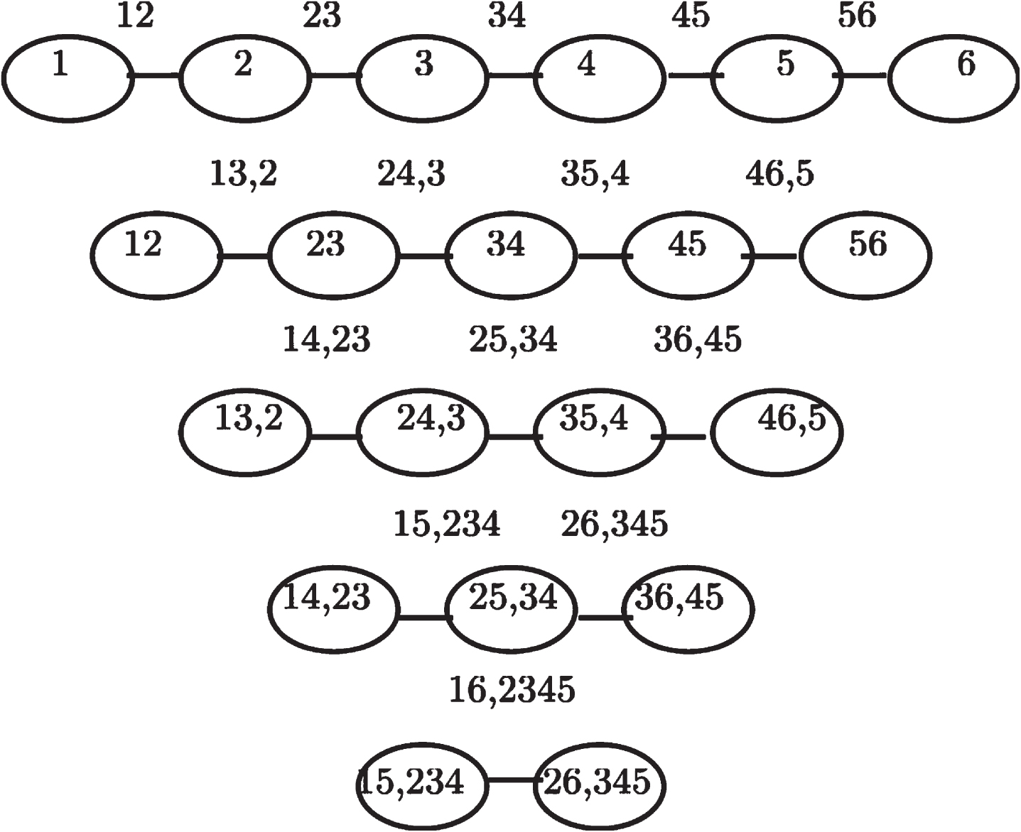
R-vines structure.

The density composition of Fig. 6 is $\begin{matrix} c F_{1} (x_{1}), . . ., F_{6} (x_{6}) = c_{12} F_{1} (x_{1}), F_{2} (x_{2}) \\ \cdot c_{23} F_{2} (x_{2}), F_{3} (x_{3}) \cdot c_{34} F_{3} (x_{3}), F_{4} (x_{4}) \\ \cdot c_{25} F_{2} (x_{2}), F_{5} (x_{5}) \cdot c_{36} F_{3} (x_{3}), F_{6} (x_{6}) \\ \cdot c_{13; 2} F (x_{1} | x_{2}), F (x_{3} | x_{2}) \\ \cdot c_{24; 3} F (x_{2} | x_{3}), F (x_{4} | x_{3}) \\ \cdot c_{26; 3} F (x_{2} | x_{3}), F (x_{6} | x_{3}) \\ \cdot c_{35; 2} F (x_{3} | x_{2}), F (x_{5} | x_{2}) \\ \cdot c_{15; 23} F (x_{1} | x_{23}), F (x_{5}, x_{23}) \\ \cdot c_{56; 23} F (x_{5} | x_{23}), F (x_{6} | x_{23}) \\ \cdot c_{46; 23} F (x_{4} | x_{23}), F (x_{6} | x_{23} \\ \cdot c_{16; 235} F (x_{1} | x_{235}), F (x_{6} | x_{235}) \\ \cdot c_{45; 236} F (x_{4} | x_{236}), F (x_{5} | x_{236}) \\ \cdot c_{14; 2356} F (x_{1} | x_{2356}), F (x_{4} | x_{2356}) \end{matrix}$ Two particular examples of regular vines have primarily been employed in financial applications. These are denoted by C-vines and D-vines, respectively. Each model explains how to decompose the density uniquely [1]. C-vines have star structures in their tree series, while D-vines have path structures [22]. A sequence of trees aids in the identification of the necessary pairs of variables and their corresponding set of conditioning variables. The C-vine and D-vine, in particular, provide an easy graphical representation that can be linked to the decomposition of the copula density function into the product of bivariate copula densities straight away [65]. Furthermore, compared to the multivariate normal distribution and other copulas, the general C-vine copula can characterise the dependence structure among collateral return series and has superior predictive performance. The general C-vine copula was proposed as a component of portfolio strategies that inventory financial providers could use to reduce default risks and improve their risk profile [89].

An R package for CDVine software includes functions and tools for statistical inference of C-vine and D-vine copulas. It includes bivariate exploratory data analysis methods, bivariate copula selection, and pair-copula family selection in a vine [74]. Furthermore, [4] has examined the dependence risk characteristics of three 20-stock portfolios from the retail, manufacturing, and gold-mining equity sectors of the Australian market in periods before, during, and after the 2008–2009 global financial crisis (GFS) using R-vine, C-vine, and D-vine. Moreover, as an extension to prior contributions in quantitative risk management, modeling non-life insurance risks in a multivariate framework was investigated. This research analyses the influence of explicit dependence modeling on capital requirements for non-life insurance losses using a D-vine copula [57]. Figure 7 shows the tree structure of the C-vine, while Fig. 8 shows the tree structure of the D-vine.

Fig. 7

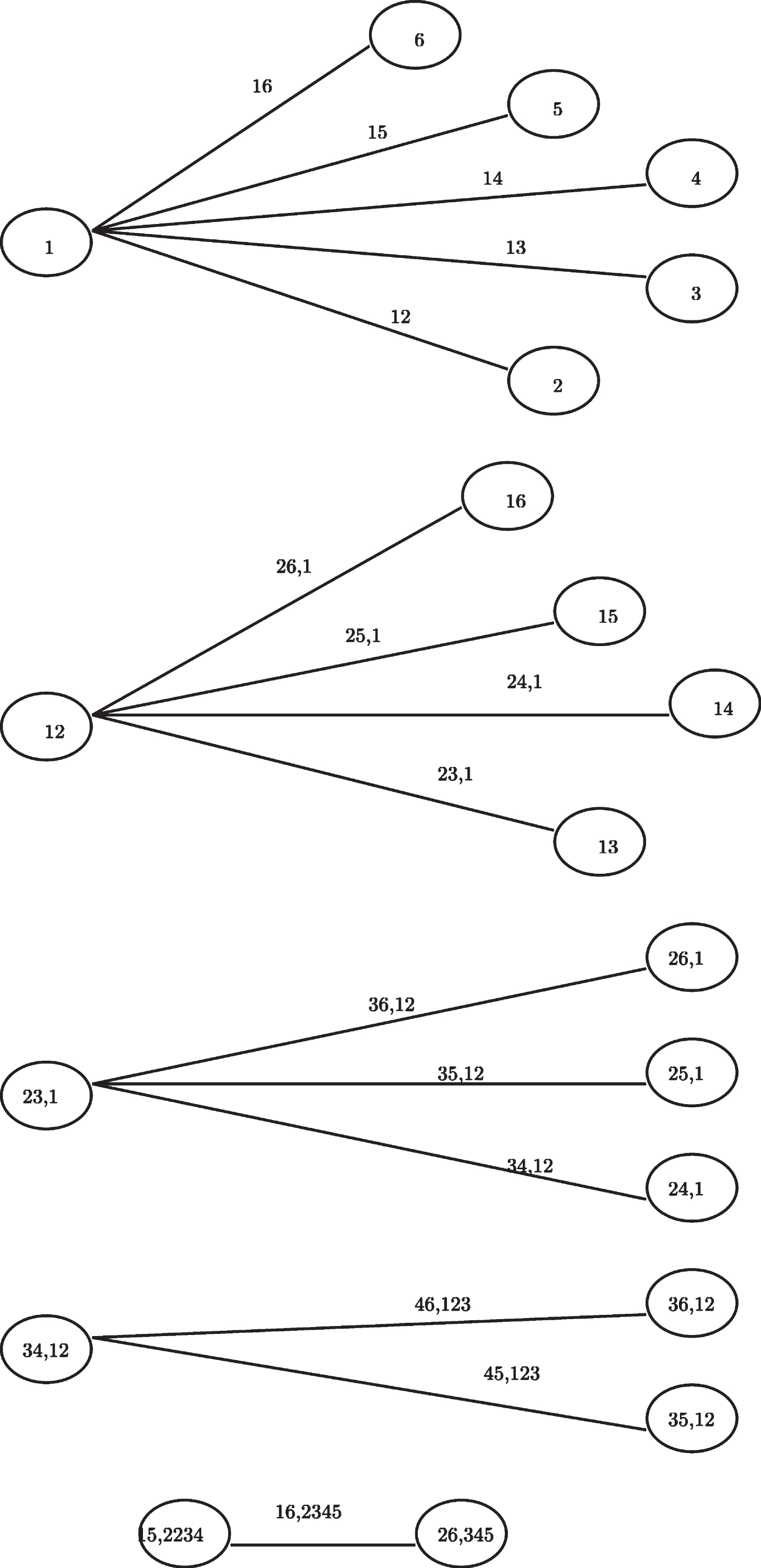
C-vines structure.

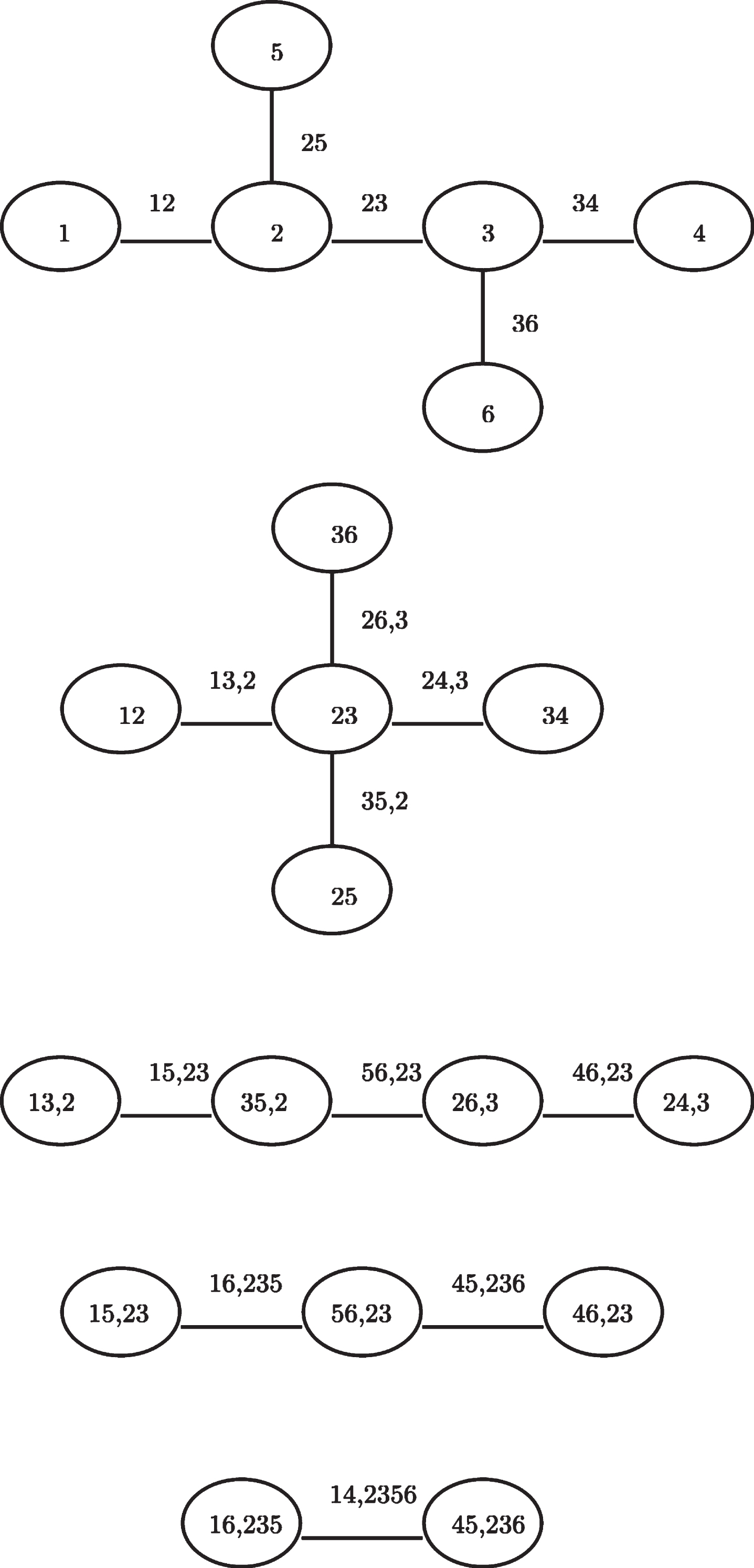
The density composition of Fig. 7 is $\begin{matrix} c F_{1} (x_{1}), . . ., F_{6} (x_{6}) = c_{12} F_{1} (x_{1}), F_{2} (x_{2}) \\ \cdot c_{13} F_{1} (x_{1}), F_{3} (x_{3}) \cdot c_{14} F_{1} (x_{1}), F_{4} (x_{4}) \\ \cdot c_{15} F_{1} (x_{1}), F_{5} (x_{5}) \cdot c_{16} F_{1} (x_{1}), F_{6} (x_{6}) \\ \cdot c_{23; 1} F (x_{2} | x_{1}), F (x_{3} | x_{1}) \\ \cdot c_{24; 1} F (x_{2} | x_{1}), F (x_{4} | x_{1}) \\ \cdot c_{25; 1} F (x_{2} | x_{1}), F (x_{5} | x_{1}) \\ \cdot c_{26; 1} F (x_{2} | x_{1}), F (x_{6} | x_{1}) \\ \cdot c_{34; 12} F (x_{3} | x_{12}), F (x_{4}, x_{12}) \\ \cdot c_{35; 12} F (x_{3} | x_{12}), F (x_{5} | x_{12}) \\ \cdot c_{36; 12} F (x_{3} | x_{12}), F (x_{6} | x_{12} \\ \cdot c_{45; 123} F (x_{4} | x_{123}), F (x_{5} | x_{123}) \\ \cdot c_{46; 123} F (x_{4} | x_{123}), F (x_{6} | x_{123}) \\ \cdot c_{56; 1234} F (x_{5} | x_{1234}), F (x_{6} | x_{1234}) . \end{matrix}$

Fig. 8

D-vines structure.

The density composition of Fig. 8 is

$\begin{matrix} c F_{1} (x_{1}), . . ., F_{6} (x_{6}) = c_{12} F_{1} (x_{1}), F_{2} (x_{2}) \\ \cdot c_{23} F_{2} (x_{2}), F_{3} (x_{3}) \cdot c_{34} F_{3} (x_{3}), F_{4} (x_{4}) \\ \cdot c_{45} F_{4} (x_{4}), F_{5} (x_{5}) \cdot c_{56} F_{5} (x_{5}), F_{6} (x_{6}) \\ \cdot c_{13; 2} F (x_{1} | x_{2}), F (x_{3} | x_{2}) \\ \cdot c_{24; 3} F (x_{2} | x_{3}), F (x_{4} | x_{3}) \\ \cdot c_{35; 4} F (x_{3} | x_{4}), F (x_{5} | x_{4}) \\ \cdot c_{46; 5} F (x_{4} | x_{5}), F (x_{6} | x_{5}) \\ \cdot c_{14; 23} F (x_{2} | x_{23}), F (x_{4}, x_{23}) \\ \cdot c_{25; 34} F (x_{2} | x_{34}), F (x_{5} | x_{34}) \\ \cdot c_{36; 45} F (x_{3} | x_{45}), F (x_{6} | x_{45} \\ \cdot c_{15; 234} F (x_{1} | x_{234}), F (x_{5} | x_{234}) \\ \cdot c_{26; 345} F (x_{2} | x_{345}), F (x_{6} | x_{345}) \\ \cdot c_{16; 2345} F (x_{1} | x_{2345}), F (x_{6} | x_{2345}) . \end{matrix}$

Maximum likelihood estimation (CML) is often used in C-vine and D-vine copula models. It is critical to have good starting values for the optimization since it will require optimization with at least n(n 1)/2 parameters. The CML approach employs the empirical probability integral transform [0,1] [33] to obtain uniform margins. This approach can be broken down into two steps:

Transform margins ${(x_{1}^{t}, . . ., x_{n}^{t})}_{t = 1}^{T}$ in uniform variables ${(u_{1}^{t}, . . ., u_{n}^{t})}_{t = 1}^{T}$ using the empirical Cumulative Distribution Functions (CDF).

Estimate the parameters of the copula: $\hat{θ} = arg max \sum_{t = 1}^{T} ln C ({\hat{U}}_{1}^{t}, . . ., {\hat{U}}_{t}^{n})$ .

6 Model validation

The goodness-of-fit (GOF) test is used to determine whether a copula or copula construction fits the data correctly. The probability integral transform (PIT) [70] and a transformation was used to create a goodness-of-fit test was introduced [10]. Two approaches based on the empirical copula and Kendall’s process, which were originally proposed by [3] for standard multivariate copula, were used in this paper [27, 35]. In the financial services industry, the recent crisis has prompted a re-evaluation of modeling. Experts in the modeling industry have released a manifesto for responsible modeling, which they are enthusiastically supporting, but the financial crisis is not the primary reason for the widespread use of financial modeling. between empirical copula ${\hat{C}}_{n}$ and the candidate parametric copula C_n. It is given by: S_n = ∫_[0,1]^dC_n (u) ²dC_n (u), where C_n is Kendall’s process given by: $\sqrt{n} (C_{n} - {\hat{C}}_{n})$ . Empirical copula ${\hat{C}}_{n}$ of the uniform data U₁, …, U_d can be expressed as: ${\hat{C}}_{n} (u) = \frac{1}{n} \sum_{i = 1}^{n} 1_{U_{i_{1}}} \leq U_{1}, . . ., U_{i_{d}} \leq U_{d}$ [36].

7 Discussion

There are two families of copula: elliptical copulas and Archimedean copulas. Both of these copulas are applied to different types of problems. For example, elliptical copulas, the Gaussian copula, are often popular in finance as they do not have upper or lower tail dependence. It is applied in a higher dimensions problem when pairwise dependencies are relatively symmetric and, more critically, extremes do not appear to occur simultaneously. As for the Archimedean copulas, they are best suited to the problem when the tail behavior of all pairings is comparable. However, as mentioned in the previous section, the elliptical and Archimedean copulas have their drawbacks. Therefore, studies were made in the previous years on how to encounter those drawbacks, resulting in more versatile and flexible approaches to copula, such as pair constructions copula, which is the PCC.

Furthermore, there exists a time frame where a general form of copula is then developed into a more flexible and versatile structure to corporate with more complex data. The literature on copula theory dates back to 1959 when Sklar used the word "copula" statistically. He derives the word copula for multivariate joint distribution that links to its one-dimensional marginal distribution. The concept of copula was introduced in the 1950’s decade, and the discovery of copula is associated with the three seminal research papers of Sklar, Fréchet, and Féron. Fréchet introduced distributions with the given marginal, which was further developed by his students, Féron and Sklar. Féron provided certain functions that coupled three-dimensional distributions with corresponding one-dimensional marginal distributions, defined on the unit cube [0, 1]. Then, in 1959, Sklar introduced functions on the unit d-a cube that relates d-dimensional distributions to their one-dimensional marginal distributions for any d > 2. Sklar also focused on the fundamental properties of these functions. Sklar then introduces the copula notion, which he names Sklar’s Theorem after.

In the 1990s, research on copulas and their applications grew primarily. The important monographs by [46] appeared in this decade and now become standard references on articles related to copula theory. The theory is about A class of m-variate distributions with given margins and m (m - 1)/2 dependence parameters, which is based on iteratively mixing conditional distributions, which is derived. At the end of this decade, the interest in the copula theory grew markedly. The growing interest is due to its applications in finance, insurance,, and risk analysis, as seen by the the frequency of published papers. With the turn of the new century, copula theory research and applications grew enormously. [5, 6] introduced the notion of a vine-dependent distribution and demonstrated the existence of such distributions. A vine is a visual representation of data that may be used to decrease the conditional independence property of Markov trees and belief nets. A vine allows the expert to specify conditional rank correlations, or more generally, conditional copula, so the information is never inconsistent.

Further significant developments and applications in the new century are rapidly building. Even though, unlike the c-vine and d-vines, the form of the r-vines can change widely based on the statistical characteristics of the structured multivariate distributions, [15] developed an analytical model to break down multivariate densities and estimating the inference of r-vines structures. [3] describes how multivariate datasets with complicated structures of dependence in the tails may be described using a chain of pair-copula acting on two variables simultaneously. Despite the above developments, the application of copulas in many fields of sciences and finance grew enormously in the second decade of the 21st century. [59] presents a Bayesian analysis of pair-copula constructions (PCCs), which outperformed several previous multivariate copula structures in modeling financial data relationships. To enable extreme events in bivariate margins independently, they use bivariate t-copulas as building pieces in a PCC.

The assessment of market risk has been the primary application area of PCC in finance. Market risk is typically measured in terms of value-at-risk (VaR) or conditional value-at-risk (cVaR). Both measures are intended to estimate the likelihood of large losses, creating a need for flexible dependency models such as pair-copula constructions. In the seminal paper [3], the PCC was used to simulate the dependency structure of a portfolio comprising two stock return indices and two bond return indices. Since then, these constructions have been used for equities [2, 9, 30, 84, 87], interest rates [9, 59, 69], exchange rates [19, 30, 52, 61, 88], electricity prices and other commodities [30, 38, 58, 68, 78, 82] and housing prices [90]. In the majority of these studies, the PCC outperforms alternative dependency models.

From a methodological standpoint, a misunderstanding of credit risk contributed to the 2008 financial crisis [17]. The Gaussian copula has conventionally been used to model the correlation structure of a credit portfolio, which has earned much condemnation, even in a non-academic context [71]. The works in [14, 29, 32] demonstrate how vine copula can generate a more consistent and precise forecast of a loan portfolio’s economic capital. In [20], a different credit risk application uses the pair-copula construction. This paper aims to calculate the probability of default (PD) for businesses. They consider a relation to a particular model based on balance sheet data, in which the equity dynamics are modeled using the D-vine.

Dalla Valle et al., [22] published a paper that described a new automated model selection and estimating approach based on graph theoretical principles. This comprehensive search approach is tested and implemented in a massive simulation study of a 16-dimensional financial data set, including international equities, fixed income, and commodity indexes. Schweizer and Sklar [74] present the R package CDVine, which includes functions and methods for statistical inference of C-vine and D-vine copulas, in a separate paper from 2013. It includes bivariate exploratory data analysis methods, bivariate copula selection, and pair-copula family selection in a vine. Shi et al., [79] proposed a copula regression for multivariate longitudinal claims to capture the distinctive aspects of policy-level insurance costs. The Tweedie double generalised linear model is used in the model to look at the semi-continuous claim costs of every coverage type, and a Gaussian copula is used to account for cross-sectional and temporal dependence among the multilevel claims.

Aside from that, portfolio optimization has made great strides since Markowitz’s [55] seminal work. After demonstrated it citerockafellar2000optimization that linear programming techniques can be used for cVaR optimization, this approach has become quite popular. Typically, scenarios are fed into the cVaR optimization. As a result, the returns on the portfolio’s instruments can have any multivariate distribution. In [53], individual asset returns are assumed to be distributed according to the skewed Student t-distribution of [44]. At the same time, a canonical vine copula is used to model their dependency structure. Compared to other models with elliptical or symmetric dependence frameworks, this model produces the best results across various statistical and economic metrics. Other papers demonstrating pair-copula constructions’ utility for portfolio optimization are [7, 21, 45]

The impact of explicit dependence modeling on capital requirements among non-life insurance losses is investigated in this paper. Throughout the process of development of copula, Regular vine (R-vine), canonical vine (C-vine), and drawable vine (D-vine) copulas were used by [4] to examine the dependence risk characteristics of three 20-stock portfolios from the retail, manufacturing, and gold-mining equity sectors of the Australian market in periods before, during, and after the global financial crisis (GFC) in 2008. In addition, [57] extends recent contributions in quantitative risk management by modeling non-life insurance risks in a multivariate framework. The latest study, which is by [16], describes how rank-based procedures for inference in copula models for continuous responses whose behavior does not depend on covariates can be adapted to the broader framework in which (possibly non-linear) regression models for the marginal responses are linked by a copula that does not depend on covariates.

Consistent with the result of other studies, [13] developed a new time-varying mixed copula in which a two-stratum process sets the dynamic weights of four unique copulas to study the extent of tail dependency in four independent quadrants. The weight of each copula is established in the two-stratum process by the relative importance of positive and negative dependence systems, followed by its historical values and adjustment processes. Each stratum’s weighting mechanism changes over time. The asymmetric tail dependencies between the stock and exchange rate markets are examined using this revised formulation. As for the latest study made last two years, Quatto et al., [67] proposed a new copula for modeling higher-order dependencies between pairs of portfolio assets, employing orthogonal polynomials to model symmetric co-kurtoses. The Gram–Charlier expansion of the Normal distribution or Gram–Charlier-like expansions of leptokurtic laws are used to describe skewness and leptokurtosis of portfolio margins.

In another study produced in 2021, the general C-vine copula can characterise the dependence structure among collateral return series and has greater predictive accuracy over the multivariate normal distribution and other copulas, according to [89]. The general C-vine copula was proposed as a component of portfolio methods that financial inventory providers may use to reduce default risks and improve their risk profile. Therefore, it is shown that copula has grown these past decades vigorously, and remarkably it is an essential tool for solving problems related to finance and insurance.

8 Conclusion

This paper can comprehensively review the development of copulas that focus on the financial field. Based on our study, various previous research supports that copulas have undergone a significant development process over these past decades. The main research findings are as follows: On the one hand, the concept of copula leads to determining the best way to solve the problem with more than one marginal distribution since it connects the marginal distribution functions. Besides, problems associated with dependence measures can also be solved efficiently using the copulas function as they are much more accurate and popular [64]. Furthermore, many copulas can help researchers determine the suitable model for solving their financial problems based on their characteristics, such as R-Vine, C-Vine, and D-Vine copulas. This will give them options to calibrate the maximum usage of the copula model to achieve the best analysis outcome.

Our paper’s findings have important implications. Our paper reveals that the development of copulas has successfully assisted financial problems that involve complicated dependence measures. For example, to study the correlation structure of a credit portfolio, researchers should consider using the Gaussian copula due to its radially symmetric factor, and it is the most popular copula for modeling association. Furthermore, to solve the market risk problem, it is recommended to use the PCC. This is because PCC can minimize dimension by pairing the variable set and creating a versatile dependency structure. This information helps future researchers to choose the appropriate copula related to the financial field. Besides that, our paper also provides knowledgeable remarks on copula from its first existence, which was first introduced by Sklar [81] when he tried to solve problems related to fundamental features of connecting d-dimensional distributions with one-dimensional marginal distributions. He then discovered that there exists a task of identifying a link between those two distributions. As a result, he introduced a copula function, which is a statistical function connecting n-dimensional distributions to their one-dimensional margins. This copula function was put under his name, which is known as Sklar’s theorem. In the first decade of the 21st century, copula keeps evolving, especially in the financial field. This is shown in the paper [3], which indicates that the extended copula, the PCC, is used to simulate the dependency structure of a portfolio of different stocks. The latest study, by Zhi et al., [89], revealed that the general C-Vine copula could characterize the dependence structure among collateral return series. This shows that the copula has grown these past decades rapidly. As an initial attempt at reviewing the development of copulas in finance, this work can be extended in several directions. First, instead of focusing on the applications in finance, this study could include the applications of copulas in other fields, such as medicine and education. For instance, in the medical research paper of [86], he discussed the simple modifications that maintain the probit assumption for marginal distributions while introducing non-normal dependence using copulas. The paper’s findings show that the Frank copula outperforms the standard bivariate probit model on the effect of insurance status on the absence of ambulatory health care expenditure. Moreover, in the education field, Gilenko and Chernova [37] discovered that to secure the positive effect of financial literacy on financial well-being, specifically via saving more actively, appropriate programs should be introduced at the early stages of education. They employed a copula-based bivariate probit-regression approach and found that the studied magnitude is substantially greater when the endogeneity effect is appropriately controlled for. Furthermore, in line with the rapid development of copula, a new update on research on copula and its application can also be included in the paper.

Footnotes

Acknowledgment

We acknowledge financial support from the Ministry of Higher Education Malaysia under the Fundamental Research Grant Scheme (FRGS) FRGS/1/2020/ STG06/UTHM/03/5.

References

Aas

, Pair-copula constructions for financial applications: A review, Econometrics 4(4) (2016), 43.

Aas

and Berg

, Models for construction of multivariate dependence–a comparison study, In Copulae and Multivariate Probability Distributions in Finance, Routledge (2013), pp. 43–64 .

Aas

, Czado

, Frigessi

and Bakken

, Pair-copula constructions of multiple dependence, Insurance: Mathematicsand Economics 44(2) (2009), 182–198.

Hernandez

J. Arreola

, Hammoudeh

, Nguyen

D.K.

, Al Janabi

M.A.

and Reboredo

J.C.

, Global financial crisis and dependence risk analysis of sector portfolios: A vine copula approach, Applied Economics 49(25) (2017), 2409–2427.

Bedford

and Cooke

R.M.

, Probability density decomposition for conditionally dependent random variables modeled by vines, Annals of Mathematics and Artificial intelligence 32(1) (2001), 245–268.

Bedford

and Cooke

R.M.

, Vines– a new graphical model fordependent random variables, The Annals of Statistics 30(4) (2002), 1031–1068.

Bekiros

, Hernandez

J.A.

, Hammoudeh

and Nguyen

D.K.

, Multivariate dependence risk and portfolio optimization: An application to mining stock portfolios, Resources Policy 46 (2015), 1–11.

Bouyé

, Durrleman

, Nikeghbali

, Riboulet

and Roncalli

, Copulas for finance-a reading guide and some applications, Available at SSRN 1032533, 2000.

Brechmann

E.C.

, Czado

and Aas

, Truncated regular vines in high dimensions with application to financial data, Canadian Journal of Statistics 40(1) (2012), 68–85.

10.

Breymann

, Dias

and Embrechts

, Dependence structures formultivariate high-frequency data in finance, Quantitative Finance 1 (2003), 1–14.

11.

Burney

and Ajaz

O. Bin

, Copulas: A historical literature review and major developments, ResearchGate, (2020), pp 2–7.

12.

Burney

and Ajaz

O. Bin

, Copulas: A historical literature review and major developments abstract, 2020.

13.

Chang

K.-L.

, A new dynamic mixture copula mechanism to examine the nonlinear and asymmetric tail dependence between stock and exchange rate returns, Computational Economics 58(4) (2021), 965–999.

14.

Changqing

, Yanlin

and Mengzhen

, Credit portfolio risk evaluation based on the pair copula var models, Journal of Finance and Economics 3(1) (2015), 15–30.

15.

Cooke

R.M.

and Kurowicka

, Uncertainty analysis and dependence modeling, Encyclopedia of Quantitative Risk Analysis and Assessment 4 (2008).

16.

Côté

M.-P.

, Genest

and Omelka

, Rank-based inferencetools for copula regression, with property and casualty insurance applications, Insurance: Mathematics and Economics 89(2019), 1–15.

17.

Crouhy

M.G.

, Jarrow

R.A.

and Turnbull

S.M.

, The subprime credit crisis of 2007, The Journal of Derivatives 16(1) (2008), 81–110.

18.

Czado

, Brechmann

E.C.

and Gruber

, Selection of vine copulas, In Copulae in Mathematical and Quantitative Finance, Springer, 2013, pp. 17–37.

19.

Czado

, Schepsmeier

and Min

, Maximum likelihood estimation of mixed c-vines with application to exchange rates, Statistical Modelling 12(3) (2012), 229–255.

20.

Dalla

, Valle, M.E. De Giuli, C. Tarantola and C. Manelli, Defaultprobability estimation via pair copula constructions, EuropeanJournal of Operational Research 249(1) (2016), 298–311.

21.

de Melo Mendes

B.V.

and Marques

D.S.

, Choosing an optimal investmentstrategy: The role of robust pair-copulas based portfolios, Emerging Markets Review 13(4) (2012), 449–464.

22.

Dissmann

, Brechmann

E.C.

, Czado

and Kurowicka

, Selecting and estimating regular vine copulae and application to financial returns, Computational Statistics & Data Analysis 59(2013), 52–69.

23.

Durante

and Sempi

, Copula theory: An introduction, InCopula Theory and Its Applications: Proceedings of the Workshop Heldin Warsaw, 25-26 September 2009, Springer, 2010, pp. 3–31.

24.

Eling

and Jung

, Risk aggregation in non-life insurance: Standard models vs. internal models, Insurance: Mathematics and Economics 95 (2020), 183–198.

25.

Embrechts

, Lindskog

and McNeil

, Modelling dependence with copulas. Rapport technique, Département de mathématiques, Institut Fédéral de Technologie de Zurich, Zurich, 14, 2001, pp. 1–50.

26.

Fang

and Madsen

, Modified gaussian pseudo-copula: Applicationsin insurance and finance, Insurance: Mathematics and Economics 53(1) (2013), 292–301.

27.

Fermanian

J.-D.

, Goodness-of-fit tests for copulas, Journal of Multivariate Analysis 95(1) (2005), 119–152.

28.

Féron

, Sur les tableaux de corrélation dont les margessont données, cas de l’espace à trois dimensions, Publ Inst Statist Univ Paris 5 (1956), 3–12.

29.

Fischer

and Jakob

, Copula-specific credit portfolio modeling, In Innovations in Quantitative Risk Management, Springer, 2015, pp. 129–145.

30.

Fischer

, Köck

, Schlüter

and Weigert

, Anempirical analysis of multivariate copula models, Quantitative Finance 9(7) (2009), 839–854.

31.

Fréchet

, Abstract sets, abstract spaces and general analysis, Mathematics Magazine 24(3) (1951), 147–155.

32.

Geidosch

and Fischer

, Application of vine copulas to credit portfolio risk modeling, Journal of Risk and Financial Management 9(2) (2016), 4.

33.

Genest

, Ghoudi

and Rivest

L.-P.

, A semiparametric estimation procedure of dependence parameters in multivariate families ofdistributions, Biometrika 82(3) (1995), 543–552.

34.

Genest

and MacKay

R.J.

, Copules archimédiennes et families de lois bidimensionnelles dont les marges sont données, Canadian Journal of Statistics 14(2) (1986), 145–159.

35.

Genest

, Quessy

J.-F.

and Rémillard

, Goodness-of-fit procedures for copula models based on the probability integral transformation, Scandinavian Journal of Statistics 33(2) (2006), 337–366.

36.

Genest

, Rémillard

and Beaudoin

, Goodness-of-fit tests for copulas: A review and a power study, Insurance: Mathematics and Economics 44(2) (2009), 199–213.

37.

Gilenko

and Chernova

, Saving behavior and financial literacy of russian high school students: An application of a copula-based bivariate probit-regression approach, Children and Youth Services Review 127 (2021), 106–122.

38.

Goodwin

B.K.

and Hungerford

, Copula-based models of systemic riskin us agriculture: Implications for crop insurance and reinsurance contracts, American Journal of Agricultural Economics 97(3) (2015), 879–896.

39.

Grønneberg

and Hjort

N.L.

, The copula information criteria, Scandinavian Journal of Statistics 41(2) (2014), 436–459.

40.

Gruber

and Czado

, Sequential bayesian model selection of regular vine copulas, Bayesian Analysis 10(4) (2015), 937–963.

41.

Haff

I.H.

, Pair-copula constructions-an inferential perspective, 2012.

42.

Haff

I.H.

, Aas

and Frigessi

, On the simplified paircopula construction—simply useful or too simplistic? Journal of Multivariate Analysis 101(5) (2010), 1296–1310.

43.

Haff

I.H.

and Segers

, Nonparametric estimation of paircopula constructions with the empirical pair-copula, Computational Statistics & Data Analysis 84 (2015), 1–13.

44.

Hansen

B.E.

, Autoregressive conditional density estimation, International Economic Review (1994), 705–730.

45.

Hernandez

J.A.

, Are oil and gas stocks from the australian market riskier than coal and uranium stocks? dependence risk analysis and portfolio optimization, Energy Economics 45 (2014), 528–536.

46.

Joe

, Families of m-variate distributions with given margins and m(m-1)/2 bivariate dependence parameters, Lecture Notes-Monograph Series (1996), 120–141.

47.

Joe

, Asymptotic efficiency of the two-stage estimation method for copula-based models, Journal of Multivariate Analysis 94(2) (2005), 401–419.

48.

Joe

, Li

and Nikoloulopoulos

A.K.

, Tail dependence functionsand vine copulas, Journal of Multivariate Analysis 101(1) (2010), 252–270.

49.

Jouanin

J.-F.

, Riboulet

and Roncalli

, Financial applicationsof copula functions, (2004), 273–301.

50.

Karava

, Financial modeling & risk management, As apart ofFinancial Modeling Course @ ALBA Graduate Business School 3(2014), 74.

51.

Kimeldori

and Sampson

, Uniform representations of bivariatedistributions, Communications in Statistics 4(7) (1975), 617–627.

52.

Maya

R.A. Loaiza

, Gomez-Gonzalez

J.E.

and Velandia

L.F. Melo

, Latin american exchange rate dependencies: A regular vine copula approach, Contemporary Economic Policy 33(3) (2015), 535–549.

53.

Low

R.K.Y.

, Alcock

, Faff

and Brailsford

, Canonical vinecopulas in the context of modern portfolio management: Are they worth it? Journal of Banking & Finance 37(8) (2013), 3085–3099.

54.

Manner

et al. Estimation and model selection of copulas with anapplication to exchange rates, Citeseer (2007).

55.

Markowitz

, Portfolio selection, The Journal of Finance 7(1) (1952), 77–91.

56.

McNeil

A.J.

and Neslehová

, Multivariate archimedean copulas, d-monotone functions and 1-norm symmetric distributions, The Annals of Statistics 37(5B) (2009), 3059–3097.

57.

Mejdoub

and Arab

M.B.

, Impact of dependence modeling of non-life insurance risks on capital requirement: D-vine copula approach, Research in International Business and Finance 45 (2018), 208–218.

58.

Mensi

, Hammoudeh

, Reboredo

J.C.

and Nguyen

D.K.

, Are sharia stocks, gold and us treasury hedges and/or safe havens for theoil-based gcc markets? Emerging Markets Review 24(2015), 101–121.

59.

Min

and Czado

, Bayesian inference for multivariate copulas using pair-copula constructions, Journal of Financial Econometrics 8(4) (2010), 511–546.

60.

Min

and Czado

, Bayesian model selection for d-vine pair-copula constructions, Canadian Journal of Statistics 39(2) (2011), 239–258.

61.

Min

and Czado

, Scomdy models based on pair-copula constructions with application to exchange rates, Computational Statistics & Data Analysis 76 (2014), 523–535.

62.

Morales-Napoles

, Counting vines. In Dependence modeling: Vinecopula handbook, World Scientific (2010), 189–218.

63.

Nagler

and Czado

, Evading the curse of dimensionality innonparametric density estimation with simplified vine copulas, Journal of Multivariate Analysis 151 (2016), 69–89.

64.

Ntwiga

D.B.

, Maritz

and Strategists

C.F.

, Copulas in finance, African Institute for Mathematical Sciences 34 (2004).

65.

Okhrin

, Ristig

and Xu

Y.-F.

, Erratum to: Copulae in high dimensions: An introduction, In Applied Quantitative Finance, Springer, 2017, pp. E1–E1.

66.

Prim

R.C.

, Shortest connection networks and some generalizations, The Bell System Technical Journal 36(6) (1957), 1389–1401.

67.

Quatto

, Vacca

and Zoia

M.G.

, A new copula for modeling portfolios with skewed, leptokurtic and high-order dependent risk factors, The North American Journal of Economics and Finance 58 (2021), 101529.

68.

Reboredo

J.C.

and Ugolini

, Downside/upside price spillovers between precious metals: A vine copula approach, The North American Journal of Economics and Finance 34 (2015), 84–102.

69.

Righi

M.B.

, Schlender

S.G.

and Ceretta

P.S.

, Pair copula constructions to determine the dependence structure of treasury bond yields, IIMB Management Review 27(4) (2015), 216–227.

70.

Rosenblatt

, Remarks on a multivariate transformation, The Annals of Mathematical Statistics 23(3) (1952), 470–472.

71.

Salmon

, The formula that killed wall street, Significance 9(1) (2012), 16–20.

72.

Scheffer

and Weiß

G.N.

, Smooth nonparametric bernstein vine copulas, Quantitative Finance 17(1) (2017), 139–156.

73.

Schellhase

and Spanhel

, Estimating non-simplified vine copulas using penalized splines, Statistics and Computing 28(2) (2018), 387–409.

74.

Schepsmeier

and Brechmann

, Modeling dependence with c-andd-vine copulas: The r package cd vine, J Stat Software 52(3) (2013), 1–27.

75.

Scheweizer

and Wolff

, Sur une mesure de dépendance pourles variables aléatoires, C R Acad Sci 283A (1976), 659–661.

76.

Schweizer

and Sklar

, Operations on distribution functions not derivable from operations on random variables, Studia Mathematica 52(1) (1974), 43–52.

77.

Schweizer

, Probabilistic metric spaces, 1983.

78.

Shen

, Odening

and Okhrin

, Can expert knowledge compensate for data scarcity in crop insurance pricing? European Review of Agricultural Economics 43(2) (2016), 237–269.

79.

Shi

, Feng

and Boucher

J.-P.

, Multilevel modeling of insurance claims using copulas, The Annals of Applied Statistics 10(2) (2016), 834–863.

80.

Shih

J.H.

and Louis

T.A.

, Inferences on the association parameter in copula models for bivariate survival data, Biometrics (1995), 1384–1399.

81.

Sklar

, Fonctions de répartition à n dimensions et leursmarges, Publications de l’Institut de Statistique del’Université de Paris 8 (1959), 229–231.

82.

Smith

M.S.

, Copula modelling of dependence in multivariate time series, International Journal of Forecasting 31(3) (2015), 815–833.

83.

Stien

and Kolbjørnsen

, D-vine creation of nongaussian random fields, The Eighth International Geostatistical Congress (2008), pp. 399–408.

84.

Weiß

G.N.

and Supper

, Forecasting liquidity-adjusted intraday value-at-risk with vine copulas, Journal of Banking & Finance 37(9) (2013), 3334–3350.

85.

Whitt

, Bivariate distributions with given marginals, The Annals of Statistics 4(6) (1976), 1280–1289.

86.

Winkelmann

, Copula bivariate probit models: With an applicationto medical expenditures, Health Economics 21(12) (2012), 1444–1455.

87.

Zhang

, Wei

, Yu

, Lai

and Peng

, Forecasting var and es of stock index portfolio: A vine copula method, Physica A: Statistical Mechanics and its Applications 416 (2014), 112–124.

88.

Zhang

, Ding

, Zhang

and Zhang

, Optimal currency composition for china’s foreign reserves: A copula approach, The World Economy 38(12) (2015), 1947–1965.

89.

Zhi

, Wang

and Xu

, Portfolio optimization for inventory financing: Copula-based approaches, Computers & Operations Research 136 (2021), 105481.

90.

Zimmer

D.M.

, Analyzing comovements in housing prices using vine copulas, Economic Inquiry 53(2) (2015), 1156–1169.