Linear feature projective geometric damped convolutional deep belief network for indoor floor planning

Abstract

Wireless localization or positioning is essential for delivering location-based services for designing location tracking systems. Traditional indoor floor planning system employs wireless signals for accurate position estimation. But these positioning schemes failed to perform position estimation effectively and accurately through many obstacles or objects. The novel technique called Linear Features Projective Geometric Damped Convolutional Deep Belief Network (LFPGDCDBN) is introduced to improve the position estimation accuracy with minimum error. The proposed LFPGDCDBN technique includes two major processes namely dimensionality reduction and position estimation. First, the dimensionality reduction process is performed by projecting the principle features using Linear Helmert–Wolf blocked Sammon projection. After the feature selection, Geometric Levenberg–Marquardt Convolutional deep belief network is employed to estimate the position of the devices with higher accuracy and minimum error. The Convolutional deep belief network uses the triangulation geometric method to identify the position of the device in an indoor positioning system. Then the Levenberg–Marquardt function is a Damped least square method to minimize the squares of the deviations between the expected and observed results at the output unit. As a result, the LFPGDCDBN increases the positioning accuracy and minimizes the error rate. Experimental MATLAB assessment is carried out with various factors such as computational time, Computational space, positioning accuracy, and positing error. The experimental results and discussion indicate that the proposed LFPGDCDBN provides improved performance in terms of achieving higher positioning accuracy and minimum error as well as computational time when compared to the existing methods. The experimental results and discussion indicate that the proposed LFPGDCDBN increases the positioning accuracy by 47% and computational time, computational complexity, and reduces the positioning error by 45%, 29%, and 74% as compared to state-of-the-art works.

Keywords

Indoor floor planning linear Helmert–Wolf blocked Sammon projection based feature selection Geometric Levenberg–Marquardt Convolutional deep belief network damped least square method

1 Introduction

With an extensively distributed Wi-Fi network and the individuality features of wireless channels, information-based positioning is crucial. As the approach requires sufficient data to be sampled at numerous access points, which consumes additional attempts and time. Many Conventional indoor positioning and localization techniques have been developed using machine learning techniques and denoted in Fig. 1. A Two-dimensional Localization Algorithm (2DimLoc) was introduced in [1] to achieve the accurate positioning of devices. But, the designed algorithm failed to consider a path loss model and influence on the RSSI, for improving the accuracy of positioning of devices. The direction of Arrival Anchor Estimation depends on Space and Frequency (DAAE-SF) [2] for indoor positioning was designed to measure actual position. The positioning system architecture was not efficient to minimize the positioning error. A particle filter-based reinforcement learning (PFRL) approach was developed in [3] for the accurate positioning of the device. But the computational space was not minimized.

Fig. 1

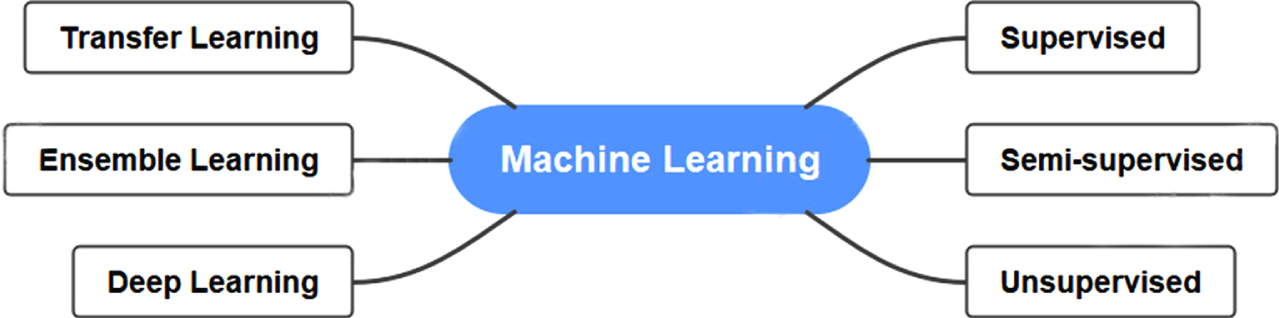
Machine learning approaches for indoor systems.

A Speed Conscious Recurrent Neural Network (SRNN) was developed in [4] for Fault Tolerant indoor localization based on RSSI (Received Signal Strength Indicator). But it failed to concentrate on the access points and automatic adjustment of access point positions to guarantee more signal coverage. A knowledge distillation into a convolutional neural network-based indoor positioning system (KD-CNN-IPS) was developed in [5]. The designed system minimizes the average positioning error but the computational space was not reduced.

Amplitude-Feature Deep Convolutional Generative Adversarial Network (AF-DCGAN) was developed in [6] for accurate indoor localization. But the computational complexity of localization was not minimized. Geomagnetic Magnetic Pattern with Convolutional Neural Networks was introduced in [7] to perform indoor localization with minimum error. But it failed to perform the localization with various orientations. Smartphone Heterogeneity Resilient Portable localization with Hidden Markov Models (SHERPA-HMM) was developed in [8] with minimal accuracy loss. But it failed to focus on improving the reliability of the framework for performing the localization. A hybrid deep-learning-based indoor localization system was introduced in [9] for improving the localization accuracy. But it failed to lessen the localization complexity. A multi-sensor tracking system was developed in [10] by integrating the Wi-Fi interface. But, it failed to design a Simultaneous Localization and Mapping (SLAM) indoor tracking algorithm to concurrently regulate the system.

The issues identified from the existing methods are lesser positioning accuracy, higher positioning error, lesser reliability, higher localization complexity, failed to regulate system, minimal signal coverage, higher path loss, higher space consumption and so on. The proposed technique concept is derived by considering the problems of these existing methods and this is highlighted in the Fig. 2. The drawbacks of these methods are effectively convinced by implementing the novel LFPGDCDBN technique. Linear Helmert–Wolf blocked Sammon projection is employed in LFPGDCDBN for principle feature selection through minimizing the sum of squares of the residuals. Geometric Levenberg–Marquardt Convolutional deep belief network is applied for position estimation.

Fig. 2

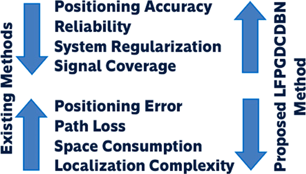
Challenges of the proposed LFPGDCDBN method.

1.1 Major contributions

To overcome the issues of existing methods, a novel LFPGDCDBN is introduced with the following contributions.

To improve the positioning accuracy of Wi-Fi devices, an LFPGDCDBN is developed based on Linear Helmert–Wolf blocked Sammon projection-based feature selection and Geometric Levenberg–Marquardt Convolutional deep belief network-based position estimation.

First, the Linear Helmert–Wolf blocked Sammon projection is employed in LFPGDCDBN for selecting the principle features from the dataset by minimizing the sum of the squares of the residuals. This process helps to minimize the computational time as well as memory consumption of an indoor localization system.

Next, Geometric Levenberg–Marquardt Convolutional deep belief network is applied to LFPGDCDBN for estimating the position of the Wi-Fi devices based on Received signal strength and path loss. The triangulation Geometric method is applied to discover the exact position of the device by calculating the intersecting point of all three medians of a triangle. Finally, the Levenberg–Marquardt function is applied to minimize the positioning error.

Finally, the experimental evaluation is conducted to compare the performance of the proposed LFPGDCDBN technique with that of existing techniques based on different metrics.

1.2 Organization of the paper

The remaining sections are arranged into different sections. In section.2, related works are discussed. Section.3 provides a brief description of the proposed LFPGDCDBN. In Section.4, experimental settings and dataset descriptions are presented. In Section.5, the results of the proposed LFPGDCDBN and existing methods are discussed with different performance metrics. Finally, Section.6 provides the conclusion of the paper.

2 Related works

A deep reinforcement learning method was developed in [11] to detect the object position and significantly reduce the time complexity. But the model failed to test the approach on single-floor and multi-floor settings. A novel Adaptive Indoor Tracking using recurrent models was developed in [12] based on the Received Signal Strength Indicator. But the other Deep Learning techniques were not applied to minimize the complexity of the network.

A weighted ensemble classifier was developed in [13] for smartphone-based indoor localization. The designed classifier increases the accuracy but the time consumption was not minimized. A novel deep learning model was introduced in [14] for the RSSI-based indoor ranging model to guarantee an efficient and autonomic calibration process. However, the computational space consumption of indoor localization was not minimized.

An efficient clustering strategy was developed in [15] for fingerprint-based positioning systems to improve positioning accuracy and minimizes storage consumption. However, the feature selection process was not performed to reduce the time consumption. Two novel deep learning-based models were developed in [16] for Wi-Fi fingerprint-based indoor localization. But it failed to use the advanced deep learning methods to further improve the accuracy of indoor localization and minimize the error.

A low-power iBeacon network was developed in [17] to perform an in-depth analysis of indoor positioning. But the machine learning or deep learning methods was not applied for improving the performance of indoor positioning. An indoor localization algorithm combining RSSI and nonmetric multidimensional scaling (NMDS) was developed in [18]. However, the designed algorithm failed to improve the positioning accuracy. Long Short-Term Memory(LSTM)-based novel indoor positioning mechanism was developed in [19]. But, the performance of indoor positioning was not improved with minimum time. A Learning-based Indoor Positioning System (LEIPS) was developed in [20]. But the positioning error was not minimized.

3 Proposal methodology

Indoor positioning has been a valuable and fashionable technology, which develops everyday lives by means of an indoor positioning system. The growth and execution of an indoor positioning system greatly depend on the technology of the wireless network. Most positioning systems implement the RSSI (received strength signal indication) received from Wi-Fi or Bluetooth AP for predicting the feasible positions of users. Due to obstacles by other indoor objects, for example, walls and furniture, the positioning accuracy and precision of an indoor positioning system have been a major challenging issue. Based on this motivation, a novel deep learning model called LFPGDCDBN is introduced for achieving higher positioning accuracy for an indoor localization system.

Figure 3 given above shows the architecture of the proposed LFPGDCDBN consists of two major processes namely dimensionality reduction and classification. First, number of features is collected from the (IPIN) 2016 competition dataset. The Helmert–Wolf blocking Targeted projection pursuit is applied for dimensionality reduction by selecting the principle features from the dataset. The principle feature selection process minimizes the computational time and overhead. With the selected principle features, the classification is performed using a Geometric Levenberg–Marquardt Convolutional deep belief network for accurate positioning of Wi-Fi devices. This process helps to improve the positioning accuracy and minimize the error. The different process of LFPGDCDBN is described in following sections.

Fig. 3

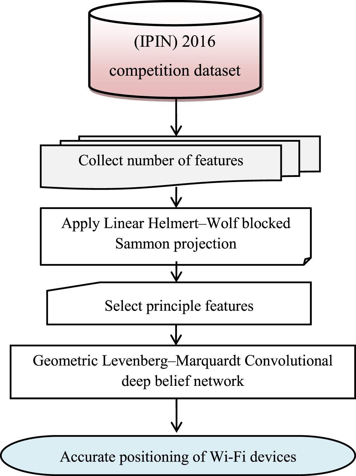
Architecture of the proposed LFPGDCDBN.

3.1 Linear Helmert–Wolf blocked Sammon projection-based feature selection

The first process of the proposed LFPGDCDBN is to perform dimensionality reduction. Since the handling of high-dimensional data is very complex in practice. As a result, the dimensionality of the input dataset becomes more complex. As the number of features increases, proportionally the number of data samples also gets enhanced. As a result, poor performance results are obtained. Therefore, the proposed technique uses Helmert–Wolf blocked Sammon projection for selecting the principle features. Feature selection presents a simple and efficient method to remove redundant and irrelevant features. Removing the redundant or irrelevant data improves learning accuracy, and reduces the computational time for the learning model high dimensional data.

Helmert–Wolf blocked Sammon projection is a dimensionality reduction technique that maps input from high-dimensional space to a lower dimensionality by trying to preserve the structure of inter-point distances. Helmert–Wolf blocking is the least squares solution method that helps to minimize the sum of the squares of the residuals (i.e. the difference between two features) for the solution of the linear model. The linear model is used to represent the relationship between two quantities (i.e. features).

Figure 4 illustrates the flow process of Linear Helmert–Wolf blocked Sammon projection for principle feature selection. Let us consider (IPIN) 2016 competition dataset and the number of features F ={ if₁, if₂, …, if_n }.

Fig. 4

Linear Helmert–Wolf blocked Sammon projection-based feature selection.

The Sammon projection maps input from the high-dimensional space to a space of lower dimensionality with help of Helmert–Wolf blocking method. A Helmert–Wolf blocking method is the least-squares method to find the optimal parameter values by minimizing the sum of squared residuals, $S = arg \min \sum_{i = 1}^{n} \sum_{j = 1}^{m} R_{ij}^{2}$ (1)

Where, $R_{ij}^{2} = \sum_{i = 1}^{n} \sum_{j = 1}^{m} | {if}_{i} - {if}_{j} |$ (2)

Where ‘S’ indicates a least-squares method, R_ij indicates a least-squares method, sum of squared residuals, arg min denotes an argument of the minimum function, |if_i - if_j| designates a Euclidean distance between two features if_i and if_j in the feature vector. The features with minimum distance are selected for the next processing. As a result, the principal features are mapped from high dimensional space into low dimensional space. $D \in [{if}_{ij} \to {if}_{s}]$ (3)

Where, D dataset, if_ij features in the high dimensional space, if_s features in the low dimensional space, → indicates a mapping function. In this way, principle features are selected to minimize the computational time. The algorithmic process of the Linear Helmert–Wolf blocked Sammon projection is expressed as follows,

Algorithm 1: Linear Helmert–Wolf blocked Sammon projection-based feature selection
Input: Dataset D, the input feature vector {if₁, if₂, …, if_n},
Output: Select principle features
Step 1: Begin
Step 2: For each feature if ∈ D
Step 3: Apply Helmert–Wolf blocking
Step 4: Compute the sum of the squares of the
residuals ‘S’
Step 5: if $(S = arg min \sum_{i = 1}^{n} \sum_{j = 1}^{m} R_{ij}^{2})$ then
Step 6: Principle Features are mapped from high
dimensional space into low dimensional space
Step 7: else
Step 8: Remove other features
Step 9: End if
Step 10: Return (dimensionality reduced features)
Step 11: End for
End

Algorithm 1 describes the step-by-step process of principle feature selection using Linear Helmert–Wolf blocked Sammon projection. The number of features is taken from the dataset. For each feature, the sum of the squares of the residuals is calculated for finding the minimum distance between the features. If the distance between the two features is minimal, then it selected as relevant and the remaining features are removed. Therefore, the significant features are selected for further processing to minimize the computational time as well as space consumption.

3.2 Geometric Levenberg–Marquardt Convolutional deep belief network

After the feature selection, the positioning of Wi-Fi devices is carried out on the indoor floors by using the Geometric Levenberg–Marquardt Convolutional deep belief network. The proposed technology determines the position of placing the Wi-Fi devices based on the Received Signal Strength Indication information.

A Geometric Levenberg–Marquardt Convolutional deep belief network is a kind of deep artificial neural network that includes various units that are highly effective for object recognition. The convolutional deep belief network includes two visible units such as input and output and hidden units. The advantage of a convolutional deep belief network is less computational complexity with the presence of many units. In addition, the convolutional deep belief network also minimizes the error. The error is the difference between original sample values and observed sample values.

Figure 5 depicts the schematic construction of the Geometric Levenberg–Marquardt Convolutional deep belief network with visible units and hidden units. In a schematic network, the input unit learns the given input data and transforms it into the hidden unit for deep analysis. Finally, the output unit displays the processed outcomes. The units are connected in a feed-forward manner with weights.

Fig. 5

Schematic structure of the Geometric Levenberg–Marquardt Convolutional deep belief network.

First, the selected features are given to the input unit of the deep belief network. $Q (t) = (\sum_{i = 1}^{n} {if}_{i} α_{ih}) + b_{c}$ (4)

Where, Q (t) indicates the input unit, α_ih indicates a weight between input and the hidden unit, if_i indicates a Select principle features, b_c denotes a bias that stored the value is +1. The input is transferred into the first hidden layer.

In the first hidden unit, let us consider the number of WI-FI devices, and the received signal strength of the devices is calculated as given below, ${ss}_{R} = [\frac{G_{t} * G_{r} * H_{t}^{2} * H_{r}^{2}}{d^{4}}] * P_{r}$ (5)

Where, ss_R designates received signal strength of the device, G_t and G_r indicates a transmitter and receiver antenna gain, $H_{t}^{2}$ symbolizes a height of AP, $H_{r}^{2}$ indicates the height of the receiver (i.e. device), d indicates the distance between sender (AP) and receiver (i.e. device), P_r denotes a transmitted signal power from the AP.

In addition, the path loss is computed and described as the signal attenuation between a transmitter and a receiver antenna. It focuses on the floors and walls that influence the RSS and is measured as given below, ${PL}_{fw} = {PL}_{0} + log (d) + {PL}_{fk} + {PL}_{wk}$ (6)

Where PL_fw denotes a path loss between the floor ‘f’ and wall ‘w’ that considers the penetration loss (PL₀) at a distance of ‘1’ meter, ‘d’ indicates the distance between transmitter and receiver, ‘PL_fk’ stand for the attenuation due to the floor ‘f’ to the ‘k^th traversed floor, ‘PL_wk’ indicates the attenuation due to the wall ‘w’ to the ‘k^th’ traversed wall correspondingly.

In the second hidden layer, triangulation is the process of finding the location (position of devices) of a point by structuring the triangles to the point from the specified points. The triangulation process is a geometric process used to measure the signal strength information and finds the exact coordinate of the Wi-Fi device. The proposed technique uses the triangulation process for determining the position of devices by forming triangles to the point from the known points.

Figure 6 illustrates the triangulation-based position of device detection. As shown in Fig. 6(a), the coordinates of the vertices (i.e. access points (APs)) of a triangle are (x₁, y₁) , (x₂, y₂) , (x₃, y₃). The centroid of a triangle (p) is determined at the intersecting point of all three medians (k₁, k₂, k₃) of a triangle. The median of the sides of a triangle is formulated as given below, $k_{1} = (\frac{x_{1} + x_{2}}{2}, \frac{y_{1} + y_{2}}{2})$ (7) $k_{2} = (\frac{x_{2} + x_{3}}{2}, \frac{y_{2} + y_{3}}{2})$ (8) $k_{3} = (\frac{x_{3} + x_{1}}{2}, \frac{y_{3} + y_{1}}{2})$ (9)

Fig. 6(a)

Triangulation based position detection.

After calculating the median of the sides of a triangle, the intersecting point of all three medians (k₁, k₂, k₃) sides of a triangle are pointed as given below, $p = (\frac{x_{1} + x_{2} + x_{3}}{3}, \frac{y_{1} + y_{2} + y_{3}}{3})$ (10)

Where, x₁, x₂, x₃ are ^′x’ coordinates of the vertices of a triangle. y₁, y₂, y₃ denotes the y coordinates of the vertices of a triangle. The centroid of a triangle point ‘p’ is taken as a fitting location (i.e. (p)) for positioning the Wi-Fi device.

The hidden unit output is formulated as given below, $H = (\sum_{i = 1}^{n} {if}_{i} * α_{ih}) + [h_{t - 1} * α_{h}]$ (11)

From (9), ‘H indicates the hidden layer output, ‘α_ih’ denotes the weight between input and the hidden unit, α_h indicates the weight of the hidden unit, h_t-1 denotes an output of the previous hidden unit. Finally, the visible output unit is given below, $Z = α_{ho} H$ (12)

Where ‘Z represents the final results of the output layer, α_ho’ represents the weight between the hidden and output unit, H denotes the output of the hidden unit. After the classification, the weight between the units gets updated by means of gradient descent in order to minimize the positioning error. ${α_{ij (t + 1)}}_{.} = α_{t} + φ [\frac{\partial log P_{r} (Z)}{\partial α}]$ (13)

From (13), α_ij(t+1) indicates an updated weight, α_t indicates a current weight, ‘φ‘ denotes a learning rate, P_r (Z) indicates a probability of results at the output unit, $\frac{\partial log P_{r} (Z)}{\partial α}$ represents the first-order iterative algorithm to find a local minimum of a function (i.e. error rate) by updating the current weight using Levenberg–Marquardt function. A Levenberg–Marquardt function is a damped least-squares method used to minimize the least squares problems i.e. the difference between the expected and observed results. $F = arg min (Z_{e} - Z)^{2}$ (14)

Where, F indicates a Levenberg–Marquardt function, Z_e represents expected positioning results, Z indicates observed positioning results. In this way, accurate positioning of the Wi-Fi device is obtained at the output unit with minimum error. The algorithmic process of the proposed Geometric Levenberg–Marquardt Convolutional deep belief network is described as given below,

Algorithm 2: Geometric Levenberg – Marquardt Convolutional deep belief network
Input: Selected principle features, Number of Wi-Fi devices, signal strength (ss_R), path loss (PL_fw)
Output: Improve the Positioning accuracy
Begin
Step 1: selected principle features are taken as input
Step 2: For each device
Step 3: Measure signal strength (ss_R) and path loss
(PL_fw) in hidden units
Step 4 : end for
Step 5: Evaluate the signal strength^′SS_R’
Step 6: Apply the triangulation process
Step 7: Find the position (p) of the device by
intersecting the point of all three medians
(k₁, k₂, k₃) sides of a triangle
Step 8: Update the weights between the units
Step 9: Levenberg–Marquardt function ‘F’ to find the minimum error ‘
Step 10: Obtain (exact position of the device) in the output unit
End

Algorithm 2 explains the step-by-step process of the positioning of the devices using the Geometric Levenberg–Marquardt Convolutional deep belief network. First, the selected features are given to the input unit. For each device, the signal strength and path loss are computed in the hidden unit. Based on the analysis, the triangulation process is applied to find the position of the device by intersecting the point of all three medians of a triangle. Finally, the weight between the units gets updated, and applies Levenberg–Marquardt function to find the minimum error. In this way, accurate positioning of the device is obtained at the output unit with minimum time.

4 Experimental settings

In this section, an experimental assessment of the proposed LFPGDCDBN technique and other five existing approaches namely Two-dimensional Localization Algorithm (2DimLoc) [1], Direction of Arrival Anchor Estimation based on Space and Frequency (DAAE-SF) [2], PFRL [3], SRNN [4], KD-CNN [5] are implemented in Python. Python is a powerful general-purpose programming language that helps to handle big data and perform complex mathematics applications. In our experimental settings, the indoor floor planning is performed using IPIN 2016 competition dataset [21, 22] is used. Multiple data have been collected from four dissimilar buildings at various timestamps. The dataset includes a variety of inbuilt sensors of smartphone-like Wi-Fi, Magnetometer, Accelerometer, Barometer, Gyroscope, and so on. The IPIN 2016 competition contains 816 access points (APs) and 26 log files out of which 17 log files are used for training. On the other hand, 9 log files are used for evaluating work testing to find the exact positioning of the device. The log files consist of five columns such as sequence number, building-id, number of floors, number of landmarks, and smartphone used to capture the data of specific log files shown in Fig. 6(b).

Fig. 6(b)

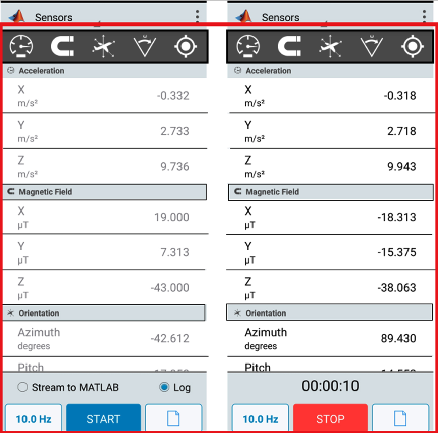
Sensor data form proposed system.

5 Performance results analysis

The performance analysis of the LFPGDCDBN technique and other five existing approaches namely Two-dimensional Localization Algorithm (2DimLoc) [1], Direction of Arrival Anchor Estimation based on Space and Frequency (DAAE-SF) [2], PFRL [3], SRNN [4], KD-CNN [5] is determined in terms of computational time, computational complexity, and positioning accuracy.

5.1 Impact of computational time

Computational time referred to the amount of time taken by an algorithm for object localization inside a building wirelessly. The lower computational time involved showed the efficiency and effectiveness of designing the method. The formula for calculating the Computational time is given below, $CT = Time (w) * Size (f)$ (15)

Where, CT indicates a computational time, Times (w) denotes an amount of time involved in object localization and ‘Size (f)’ represents the number of floors. It is measured in the unit of milliseconds (ms). Table 1 (a & b) and fig 7 illustrate the comparative analysis of computational time for proposed LFPGDCDBN network parameters and five existing methods namely 2DimLoc [1], Direction of Arrival Anchor Estimation based on Space and Frequency (DAAE-SF) [2], PFRL [3], SRNN [4], KD-CNN [5]. The x-axis depicts number of trials and the y-axis signifies the performance of computational time for positioning the device.

Table 1(a)

Computational time

Number	Computational Time (ms)
of trials	2DimLoc	DAAE-SF	PFRL	SRNN	KD-CNN-IPS	LFPGDCDBN
1	0.18	0.16	0.16	0.15	0.14	0.11
2	0.61	0.39	0.43	0.26	0.24	0.17
3	0.72	0.55	0.56	0.38	0.34	0.21
4	0.95	0.71	0.75	0.56	0.48	0.27
5	1.15	0.85	0.84	0.68	0.57	0.38
6	1.45	0.90	1.20	0.79	0.69	0.47
7	1.75	1.15	1.42	0.85	0.81	0.66
8	1.80	1.45	1.60	0.96	0.92	0.74
9	1.95	1.60	1.75	1.12	1.06	0.83
10	2.25	1.90	2.09	1.5	1.35	0.93

Table 1(b)

Proposed LFPGDCDBN parameters

Dataset	Number of Hidden Layers	Number of Hidden Layer Nodes	Pretrain Learning Rates	Fine-Tune Learning Rates
Ref.no [21]	4	310×100×100	0.01	0.001
Ref.no [22]	4	280×100×100	0.05	0.003

The observed results show the proposed LFPGDCDBN is capable of providing less computational time for positioning the device than the conventional methods. The reason behind the improvement is because of using the Linear Helmert–Wolf blocked Sammon projection to select the relevant features. The number of features is taken from the dataset. The sum of squared residuals is calculated for finding the minimum distance between the features. When the distance between features are lesser, the features are selected and the other features are removed. As shown in Fig. 7, ten results are observed. The average of ten comparison results indicates that the computational time using LFPGDCDBN is considerably reduced by 63%,51%,55% 35%, and 29% when compared to five existing methods namely [1 –5] respectively.

Fig. 7

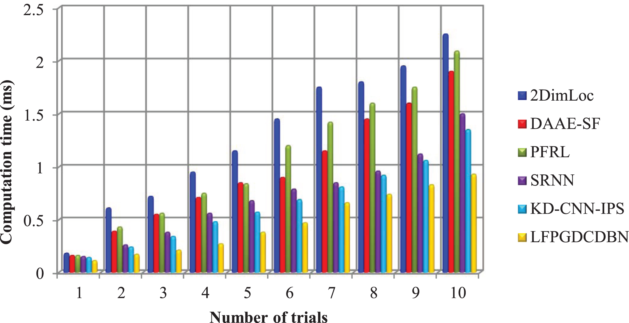
Comparison of computational time.

5.2 Impact of computational space

Computational space refers to the amount of memory consumed by algorithms for object localization in indoor floor planning. The computational space is mathematically formulated as given below, $CS = MEM (w) * Size (f)$ (16)

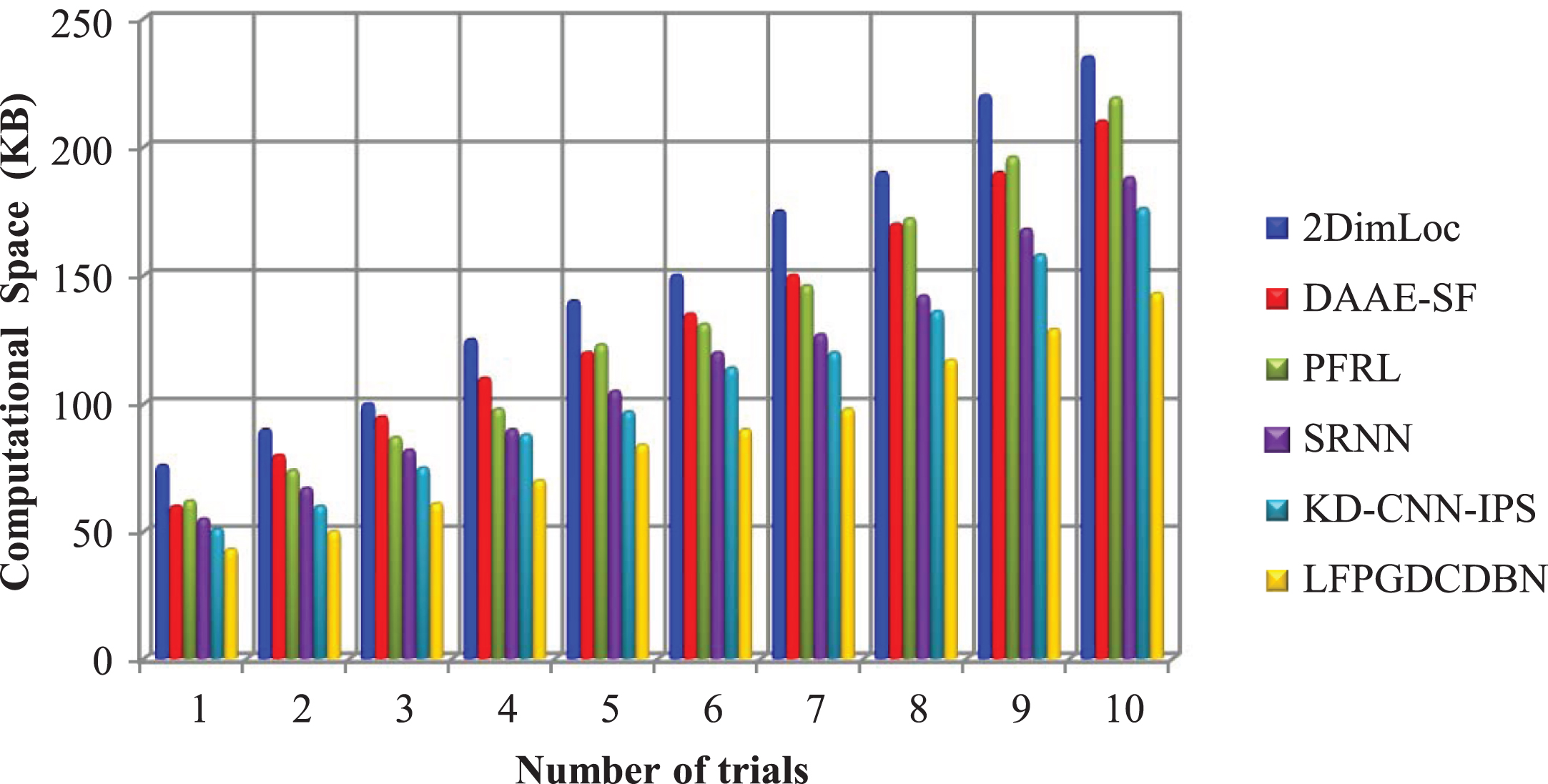
Where, CS denotes a computational space, MEM (w)’ represents the memory consumed for localization of objects, ‘Size (f) denotes the number of floors considered for conducting the experimental evaluation. The overall computational space is measured in terms of kilobytes (KB). Table 2 and Fig. 8 given above provide the tabular and graphical representation of computational space. From the Fig. 8 horizontal axis represents the number of trials ranging between 1 and 10. On the other hand, the vertical axis denotes the performance of computational space measured in terms of kilobytes (KB). Also from the above Fig. urative representation, the computational space is found to be minimized than the other existing methods. The reason behind this improvement was due to the selection of principle features from the dataset and removing the other features.

Table 2

Computational space

Number of trials	Computational Space (KB)
	2DimLoc	DAAE-SF	PFRL	SRNN	KD-CNN-IPS	LFPGDCDBN
1	76	60	62	55	51	43
2	90	80	74	67	60	50
3	100	95	87	82	75	61
4	125	110	98	90	88	70
5	140	120	123	105	97	84
6	150	135	131	120	114	90
7	175	150	146	127	120	98
8	190	170	172	142	136	117
9	220	190	196	168	158	129
10	235	210	219	188	176	143

Fig. 8

Comparison of computational space.

The reason behind this improvement is due to the selection of principle features from the dataset and removing the other features using Linear Helmert–Wolf blocked Sammon projection. The projection function maps the principle feature from high dimensional space into low dimensional space. Therefore, the positioning of various devices is performed with less number of features resulting in minimizing the computational space. The performance of computational space is considerably minimized by 41%, 33%, 32%, 23%, and 18% using LFPGDCDBN when compared to existing 2DimLoc [1], DAAE-SF [2], PFRL [3], SRNN [4], and KD-CNN [5] respectively.

5.3 Impact of positioning accuracy

It is measured to find how the proposed algorithm accurately detects the positioning of the device to the number of the device taken as input. The formula is expressed as follows,

$PosAcc = [\frac{No . of devices accuratelypositioned in thefloor}{No . of devices}] * 100$ (17)

Where PosAcc represents theWI-FI device positioning accuracy is measured in terms of percentage (%).

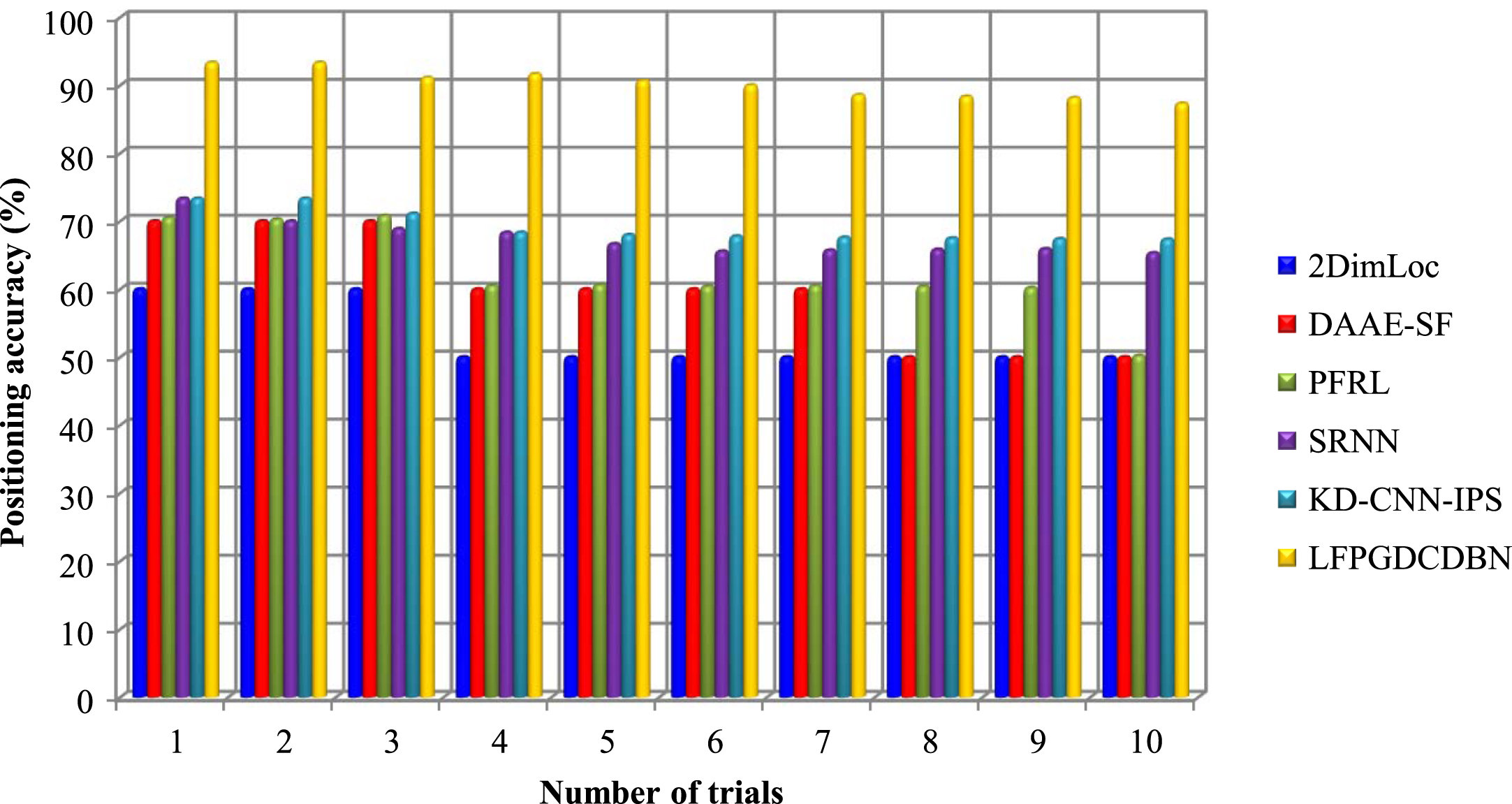
Table 3 and Fig. 9 reveal the comparative analysis of positioning accuracy using six different methods namely LFPGDCDBN, 2DimLoc [1], DAAE-SF [2], PFRL [3], SRNN [4], and KD-CNN [5] respectively. The x-axis denotes the number of trials and y-axis represents the positioning accuracy. The observed results indicate that the positioning accuracy of LFPGDCDBN is found to be higher when compared to existing methods. This is because of applying the Geometric Levenberg–Marquardt Convolutional deep belief network. First, the selected features and the device are given to the input unit. For each device, the signal strength and path loss are computed in the hidden unit. The triangulation process identifies the exact positioning of device by intersecting the point of all three medians of a triangle. By this way, LFPGDCDBN achieves higher positioning accuracy. The observed performance results confirm that the accuracy of LFPGDCDBN is significantly improved by 71%, 53%,4 6%, 34%, and 31% when compared to [1 –5] respectively.

Table 3

Positioning accuracy

Number of trials	Positioning Accuracy (%)
	2DimLoc	DAAE-SF	PFRL	SRNN	KD-CNN-IPS	LFPGDCDBN
1	60	70	70.5	73.33	73.33	93.33
2	60	70	70.25	70	73.33	93.33
3	60	70	70.8	68.88	71.11	91.11
4	50	60	60.5	68.33	68.33	91.66
5	50	60	60.6	66.66	68	90.66
6	50	60	60.4	65.55	67.77	90
7	50	60	60.5	65.71	67.61	88.57
8	50	50	60.4	65.83	67.5	88.33
9	50	50	60.2	65.92	67.40	88.14
10	50	50	50.2	65.33	67.33	87.33

Fig. 9

Comparison of positioning accuracy.

5.4 Impact of positioning error

It is measured to find how the proposed algorithm incorrectly detects the positioning of the device to the number of the device taken as input. The formula for calculating the error rate is given below,

${Pos}_{AER} = [\frac{No . of devices incorrectlypositioned in the floor}{No . of devices}] * 100$ (18)

Where, Pos_AER represents theWI-FI device positioning error is measured in terms of percentage (%).

Table 4 and Fig. 10 provide the overall performance results of positioning error regarding a number of trials with the number of Wi-Fi devices. The x-axis denotes the number of trials and y-axis represents the positioning error. The overall results indicate that the positioning error using LFPGDCDBN is minimized than the existing techniques. The most significant reason is application of Levenberg–Marquardt function.

Table 4

Positioning error

Number of trials	Positioning Error (%)
	2DimLoc	DAAE-SF	PFRL	SRNN	KD-CNN-IPS	LFPGDCDBN
1	40	30	29.5	26.66	26.66	6.66
2	40	30	29.75	30	26.66	6.66
3	40	30	29.2	31.11	28.88	8.88
4	50	40	39.5	31.66	31.66	8.33
5	50	40	39.4	33.33	32	9.33
6	50	40	39.6	34.44	32.22	10
7	50	40	39.5	34.28	32.38	11.42
8	50	50	39.6	34.16	32.5	11.66
9	50	50	39.8	34.07	32.59	11.85
10	50	50	49.8	34.66	32.66	12.66

Fig. 10

Comparison of positioning error.

The proposed technology determines the position of placing the Wi-Fi devices based on the Received Signal Strength Indication information. This helps to improve the accurate positioning of the device and minimize the error. The average of ten results indicates that the error during the positioning of Wi-Fi devices is said to be minimized by 79%, 76%, 74%, 70%, and 69% when compared to existing 2DimLoc [1], DAAE-SF [2], PFRL [3], SRNN [4] and KD-CNN [5] respectively.

6 Conclusions

In this work, a novel fast indoor localization scheme based on a convolutional deep belief neural network called LFPGDCDBN is proposed for the accurate positioning of Wi-Fi devices with minimum error and computational time. The LFPGDCDBN first performs the feature selection from the dataset using linear Helmert–Wolf blocked Sammon projection method. The linear projection method finds the significant features and removes the other features minimizing the computational time as well as memory consumption. Followed by, Geometric Levenberg-Marquardt Convolutional deep belief network is used for positioning of the Wi-Fi devices based on the signal strength and path loss model. The experimental assessment is conducted on various metrics such as computational time, Computational space, positioning accuracy, and positing error with respect to a number of trials and the Wi-Fi devices. The discussed results have revealed that the LFPGDCDBN technique has considerably improved the performance of positioning accuracy, and minimizes the error, time as well as space consumption than the existing methods. In future work, the proposed LFPGDCDBN technique is further implemented to obtain security and privacy with a higher accuracy and minimum error by using fast indoor localization scheme based on convolutional deep belief neural network. We also plan to test the proposed model on different data-sets along with increasing the network size.

References

Hang

, Huixia

, Jian

, Min

Indoor positioning system based on particle swarm optimization algorithm, , Measurement 134 (2019), 908–913. [CrossRef]

Alessandro

, Giovanni

, Stefano

, Marco

, Giuseppe

2-D DoA anchor suitable for indoor positioning systems based on space and frequency diversity for legacy WLAN,, IEEE Microwave and Wireless Components Letters 28(7) (2018), 627–629.[CrossRef]

Jose

, Zhongliang

, Torsten

, Zan

A particle filter-based reinforcement learning approach for reliable wireless indoor positioning, IEEE Journal on Selected Areas in Communications 37(11) (2019), 2457–2473.[CrossRef]

Pothuri

, Veena

Fault-Tolerant indoor localization based on speed conscious recurrent neural network using Kullback –Leibler divergence, Peer-to-Peer Networking and Applications 15 (2022),1370–1384.[CrossRef]

Aqilah

, Yin

, Chee

A fast indoor positioning using a knowledge-distilled convolutional neural network (KD-CNN), IEEE Access 10 (2022),65326–65338.[CrossRef]

Yue

, Ruizhi

, Liang

, Wei

, Yuan

, Haitao

H-WPS: Hybrid wireless positioning system using an enhanced Wi-Fi FTM/RSSI/MEMS sensors integration approach, IEEE Internet of Things Journal 9(14) (2022),11827–11842.[CrossRef]

Imran

, Mingyu

, Soojung

, Yongwan

MINLOC: Magnetic field patterns-based indoor localization using convolutional neural networks, IEEE Access 8 (2020), 66213–66227.[CrossRef]

Saideep

, Sudeep

, Branislav

, Qi

A Hidden Markov Model based smartphone heterogeneity resilient portable indoor localization framework,,Journal of Systems Architecture 108 (2020),1–12.[CrossRef]

Hamada

, Ahmed

, Hirozumi

A robust and accurate indoor localization using learning-based fusion of Wi-Fi RTT and RSSI,, Sensors 22(7) (2022),1–22.[CrossRef]

10.

Miguel

, Luis

, Ismael

A smartphone-based multimodal indoor tracking system, , Information Fusion 76 (2021),36–45.[CrossRef]

11.

Fei

, Jin

, Tingyang

, Chun-His

, Jinbo

A bisection reinforcement learning approach to 3-D indoor localization, IEEE Internet of Things Journal 8(8) (2021),6519–6535.[CrossRef]

12.

Alberto

, Gustavo

, David

, Federico

Recurrent model for wireless indoor tracking and positioning recovering using generative networks, IEEE Sensors Journal 20(6) (2022),3356–3365.[CrossRef]

13.

Priya

, Chandreyee

, Mausam

, Dip

, Sanghamitra

Novel weighted ensemble classifier for smartphone based indoor localization, Expert Systems with Applications 164 (2021),1–13.[CrossRef]

14.

Amir

, Ghofrane

, Maher

, Faouzi

A new deep learning-based distance and position estimation model for range-based indoor localization systems, Ad Hoc Networks 114 (2021), 1–12.[CrossRef]

15.

Pampa

, Supriya

, Keshav

, Samiran

, Nilkantha

, Xinheng

An efficient clustering with robust outlier mitigation for Wi-Fi fingerprint based indoor positioning, Applied Soft Computing 109 (2021), 1–15.[CrossRef]

16.

Weizhu

, Fabrice

, Franck

Supervised and semi-supervised deep probabilistic models for indoor positioning problems, [CrossRef], Neurocomputing 435 (2021), 228–238.[CrossRef]

17.

Xiaona

, Shufang

, Shuaiheng

Low-power indoor positioning algorithm based on iBeacon network, [CrossRef], Complexity 2021 (2021), 1–10.[CrossRef]

18.

Shuxia

Wireless network indoor positioning method using nonmetric multidimensional scaling and RSSI in the internet of things environment, Mathematical Problems in Engineering 2020 (2020), 1–7.[CrossRef]

19.

Halgurd

Maghdid Kayhan

Abdulbasit

Ali

Pranav

Danda

Enabling accurate indoor localization for different platforms for smart cities using a transfer learning algorithm, Internet technology letter 5(1) (2022), 1–6.[CrossRef]

20.

Szu-Yin

, Fang-Yie

, Chia-Yin

, Ming-Chien

A deep learning-based indoor-positioning approach using received strength signal indication and carrying mode information, [CrossRef], Concurrency and Computation Practice Experience33(23) (2020), 1–12.[CrossRef]

21.

Sushil

, Vinod

Smartphone based improved floor determination technique for multi-floor buildings, 2018 Proceedings of the World Congress on Engineering 1 (2018), 4–6.

22.

Zhao

, Qin

, Guo

, Wang

Indoor floor localization based on multi-intelligent sensors, ISPRS Int J Geo-Inf10 (2021),6. https://dx.doi.org/10.3390/ijgi10010006 .