
Abstract
The main function of the internal control department of a bank is to inspect the banking operations to see if they are performed in accordance with the regulations and bank policies. To accomplish this, they pick up a number of operations that are selected randomly or by some rule and, inspect those operations according to some predetermined check lists. If they find any discrepancies where the number of such discrepancies are in the magnitude of several hundreds, they inform the corresponding department (usually bank branches) and ask them for a correction (if it can be done) or an explanation. In this study, we take up a real-life project carried out under our supervisory where the aim was to develop a set of predictive models that would highlight which operations of the credit department are more likely to bear some problems. This multi-classification problem was very challenging since the number of classes were enormous and some class values were observed only a few times. After providing a detailed description of the problem we attacked, we describe the detailed discussions which in the end made us to develop six different models. For the modeling, we used the logistic regression algorithm as it was preferred by our partner bank. We show that these models have Gini values of 51 per cent on the average which is quite satisfactory as compared to sector practices. We also show that the average lift of the models is 3.32 if the inspectors were to inspect as many credits as the number of actual problematic credits.
Introduction
In banking one of the back-office departments is the internal control (IC) department where the main function is, as the name implies, controlling the operations of the bank internally. The IC inspectors perform their inspections for two main purposes: to check the compliance to the rules set by the Central Banking Regulation Office (CBRO) and, check the suitability to the bank strategies and polices. The controls can be made on several bank departments including credit sales, administrative operations, treasury, human resources, financial operations, and general banking operations [1]. Among these the credit sales take the most time of the IC inspectors and thus, in this study, we wanted to focus on this department.
In credit departments there are a lot of detailed rules for proper credit issuing where the process is started by the portfolio managers (PM) at the branches and continued at the central operations (COPS). The branch and COPS managers are also responsible for the processes, and they check and approve the credits at some check points of the workflow. The IC department of one of the largest Turkish banks for which we carried out this project, has had defined more than 100 rule based scenarios to check the compatibility of the credits issued to the CBRO rules (e.g. did the customer signed the general credit usage agreement and is the signature still valid (agreements are made for some time period), or, was a minimum 25 per cent down payment taken for an automotive loan, etc), or bank policies (e.g. was enough first quality collateral taken from the customer against the credit amount, etc.).
Each scenario is a control aiming at finding a discrepancy among several possible discrepancies that can be observed at a specific point in the workflow. A scenario starts with a report obtained by a query on the database listing the discrepancies from the standard credit issuing process. Some of these reports include too many entries and it is not possible to inspect all of them closely. At this point, the inspectors work on a sample and typically the credits having the highest amounts take place in these samples. If at the end of the inspection, the inspectors decide that there is an incompatibility to the rules or unsuitability to the bank polices, they send it to the branch asking for a correction (if possible) or an explanation (sometimes PMs get special permission for that credit from a manager at the headquarters and although they included it in the workflow, the inspector did not see it or sometimes, they simply forget to include it, in which case the inspector has no chance to know it).
In this study, we aim at developing predictive models that can predict the problematic credits better than inspecting the credits with the highest amounts. This will not only help a more proper operation of the bank as a whole, but also increase the performance of the IC department. This is because, if the discrepancies determined by the IC inspectors are really indicating an incompatibility, IC department is regarded as more successful.
Predictive modeling is also known as classification where we try to predict which one of the class values that the target variable will take [2]. If the target variable takes only two values (e.g positive-negative, good-bad, 1-0), it is called the binary classification. In the literature it is possible to find thousands of papers discussing the applications of binary classification [3–5].
Note that, the exact formulation of the prediction problem of the IC department will be a multi-class classification problem [6] where the number of classes will be in the magnitude of several hundred (the number of different scenarios is above 100 and in each scenario about five-six different discrepancies can be observed). When the number of classes is too large, developing a good performing model is really a challenging task. Actually, multi-classification problems are not new and there have been many applications of them in real life. However, although the binary classification problems are well studied and there have been many successful algorithms to solve them, until recently, there were not quite satisfactory algorithms for multi-classification problems. Traditionally they were approached by using binary classifiers recursively where one class label is compared to all other labels or all labels are compared to all other labels [7, 8]. Boosting methods [9, 10] or random forests [11] were also used for multi-classification. Recently, with the advances in neural networks, the techniques known as deep neural networks or deep learning have proven to show superior performances in multi-classification problems [12–14]. On the other hand, multi-classification problems are usually coupled with severe class imbalance problem which in turn increases the problem complexity even further [15].
Because of big volumes of data and large number of customers, the banking has been one of the pioneering sectors for data science applications. It is possible to find a lot of papers on banking applications in the literature where most of them are related with the marketing department [16–18] or the credit risk prediction [19–22]. Perhaps card or transactional fraud detection takes the third place [23–27] followed by some others including ATM/Branch location and cash management optimization [28–31] and, collection and early warning [32, 33].
However, to the best of our knowledge there has been no study directly aiming at the optimization of IC department functions. Thus, when we were consulted for such an efficiency tool for the IC department, we could not find any other study to get some ideas from. Consequently, we had to make a very detailed analysis and come out with a novel and useful idea. We hope other practitioners can benefit from our ideas in developing better models in the future. We also hope this will be one of the very first studies aiming at filling an important gap in the literature.
The contributions of this study to the literature can be itemized as follows. First of all, our study is the first study attempting to develop a predictive model for the IC department of a bank. Secondly, we describe the case study in detail and how we face with a classification problem with hundreds of classes. Thirdly, we describe the discussions and alternative ideas of how a complicated classification problem of IC departments can be handled. Lastly, we make a suggestion of business process re-engineering to increase the work efficiency of the IC department.
Outline of the remainder of this paper is as follows: in the next section we explain the functioning of the IC department in more detail and make it clear why predictive modeling is needed and how it can help to increase the performance of the department. Then, in the third section, we explain the solution approach we take up in this study. The target definition and the number and type of models to be developed are all discussed here. In the fourth section, after introducing the main steps of model building, we present the description and performance of the models developed. In the final section (section 5), we summarize the study and its main conclusions. We also discuss the limitations of this study, provide some suggestions for a better functioning IC department and indicate some potential future studies.
Work and problem definition
In this section we describe the functioning of the IC department in more detail. The sub department responsible for the credits control had two teams where one team has been inspecting the retail (personal) credits and the other team has been inspecting the SME and commercial credits. Each team has been using 100 + scenarios to perform their inspections. Most of these scenarios were applied every month while a few of them had a quarter or year periodicity. The scenarios were shared by the inspectors and each inspector knew her or his monthly inspection schedule. The list of the scenarios is mostly stationary but throughout time some could become void because of new IT developments, or some new scenarios could be needed because of new products and/or regulation/policy changes.
Each scenario starts with a list of credits taken from the database based on some rules. Sometimes this list contains only a few lines so that the inspector can inspect all of them. But sometimes the list is too long, and it is not possible to inspect all of them in the limited time they can devote to that scenario. In such cases, the inspectors take a sample using a simple logic where the main criterion is the credit amount. They preferred to inspect credits with high amounts which is understandable since in this case possible losses from inconveniently issued credits can be minimized. But this approach bears some problems in several aspects: Firstly, the same high amount credits can take place in the samples of different scenarios and thus, they are inspected again and again. Secondly, the parties involved in credit issuing (PMs, COPS, managers) are normally more careful in high amounted credits which decreases the chances of finding any problems and thus thirdly, it contradicts the success criteria of the IC department, where, the more problems they can find, the more successful they will be.
Some of the scenarios that need sampling are related with the existence and eligibility/quality of the collaterals used against the credit. One can think determining such discrepancies will be easy by some database queries or they can be forbidden systematically but unfortunately this is not the case because of the complicated conversion rules between different collateral qualities and some other reasons. Consequently, such scenarios consume lots of inspectors’ time.
Going back to scenario inspections; after having the list or sample of the credits to be inspected, the inspectors check their suitability to the standard way of doing business limited to the scope of that control point. If a credit does not look to be a standard issuing, they check the banking system if there is any explanation provided for that discrepancy (like an email confirmation from managers). For those credits where there is no explanation, they arrange a form questioning what has been going on and send it to the bank branch where that credit was issued. The branches should answer these forms within a specified time (typically one week) where they can either include the document explaining the discrepancy or they can claim that the document has been already in the system (which means the inspector was not careful in inspection) or they can say they will take a corrective action (if possible) if they are given some additional time (usually 10 days). In Fig. 1 we tried to illustrate this work flow.
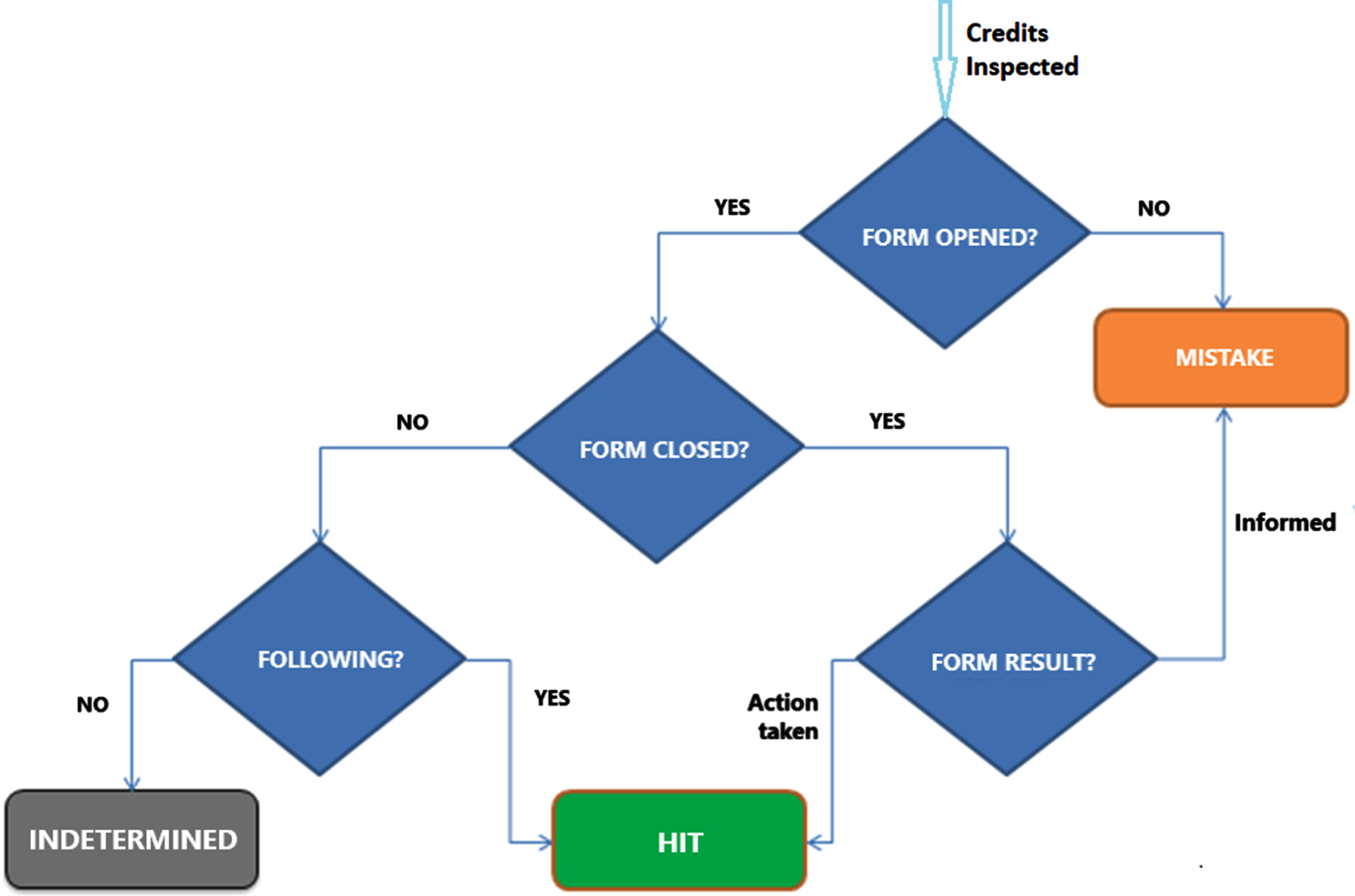
Inspection flow diagram.
The inspector receiving the answer makes a judgement and either closes the form (FORM RESULT) or keep it open so that the corrections can be followed up (FOLLOWING). The form result can either be Informed which means the document explaining the discrepancy has already been in the system or Action Taken which means either the previously forgotten document is added to the system, or a quick corrective action is taken. This latter case was labeled as a success of the inspector (
The scope of this study is to learn from previous successes and mistakes of the inspectors and develop predictive models for those scenarios where there is a need to take samples for inspection. The sole aim is to increase the success rate of the inspectors.
As a first step of the project, we have investigated the scope and aim of all 100 + scenarios. During this analysis we found out that sampling was needed for the 49 scenarios and the scope of this study is thus limited to those scenarios. Then, we have discussed if we should, or, can develop 49 predictive models, one for each of these scenarios. After long discussions we have concluded that we cannot develop 49 models for two reasons: First, we would not have enough positive (problematic) examples for some scenarios and second, it would not be easy to develop and maintain so many models. We have also concluded that we should not have a separate model for each scenario since throughout time some of them could become out of date or some new scenarios requiring predictive modeling could come out. So, it would be nice to have fewer models, but how?
To have fewer models two ideas were compared to each other. According to the first idea, scenarios could be grouped based on their similarity, in which case there would be too few positive (HIT) examples in some groups and there would be uncertainty when a new scenario which is unsimilar to any existing group is defined. According to the second idea, we wanted to deep dive and classify the discrepancies (incompatibilities, problems) across all scenarios. This one attracted more interest and we went over it. In the end, we determined that the inspectors were mainly looking for discrepancies in the following six groups: CD: collateral deficiency (e.g., lack of signature, lack of spouse approval, missing collateral-credit attachment), CQ: collateral quality (e.g., incorrect collateral quality conversion, signature by pencil), DD: other documents deficiency (e.g., lack of special approvals, expertise reports), DQ: other documents quality (e.g., aval suitability), LA: lack of attention (other unconscious mistakes of the personnel), IM: intentional mistake (other conscious mistakes of the personnel due to the pressure of reaching monthly goals or close relationship with the customer).
To develop models for each of these six discrepancy groups, it was argued that different data sources could be used: Information about the customers, information about the specific credit issued, mistake statistics of the related personnel and the bank branch. As a result, we decided to have four different datamarts (a datamart is a datawarehouse table). After detailed discussions, it was concluded that the number of variables in these datamarts would be 53, 60, 30 and 13 respectively.
Among these LA and IM models can be a bit more complicated than the others since in their occurrence more than one personnel might be involved and, in their modeling this should also be taken into account. Not only the statistics of the PM but also the statistics of the COPS personnel and sometimes the managers should also be considered.
As for any predictive model, we need a clear definition of the target variable. For any specific scenario, as also illustrated in Fig. 1, those credits that are opened a form and action taken or those for which some time is requested by branch for correction are labeled as target = 1 (HIT in Fig. 1) and those forms which are mistakenly opened and those credits for which no form was opened are labeled as target = 0 (MISTAKE in Fig. 1). On the other hand, those forms for which the response from the branch were not received yet are labeled as INDETERMINED and are left out of the model learning process.
We have to note that, some of the scenarios are related with more than one of the above six models, in other words, the discrepancies that they try to find fall into more than one of the above groups. If this was the case, the target variable should be set to 1 for all models where the scenario was a HIT. This means, the same credit can take place as target 1 in more than one model, and still, it can take place as target 0 in some other models. Also, since the same scenario might have more than one model score, we need a mechanism of how to use multiple scores. Calculating the average score or taking the maximum one, are two alternative approaches. After discussions we decided that using the maximum is more reasonable since having a high score in one of the models should be a good enough reason for the inspection.
Another issue is deciding the timing of the model scoring. One approach was scoring the credits as soon as they are issued and another one, to score them just before the actual inspections. Obviously for credit or customer related variables, using their values at the time of credit issuing is more reasonable. On the other hand, for the personnel and branch statistics, an extended time period could be more useful, however, after some discussions we have concluded that it is better not to complicate things and score the scenarios at the time of credit issuing.
Model development
In this section, first we provide a short analysis of the data and then, we introduce the description of the modeling steps we have gone through followed by a short information on the logistic regression algorithm which was preferred for this study. Then, we provide the performances of the six models developed. Afterwards, we provide a short description of the main kind of variables that took place in these models.
Only the results of the models related with the retail line of business will take place in this report.
Data analysis
For the modeling, four months data from recent period is used. The number of Hits, Mistakes and Indetermined cases per modeling subject are given in Table 1.
Summary of recent past inspection data
Summary of recent past inspection data
The ratio of Hits to the total number of Hits and Mistakes is highly small resulting in a class imbalance problem. The imbalance is larger in IM, LA and CQ which means developing good performing models for them might be harder. On the other hand, the size of the training set could be a more important problem and, in our case, unfortunately for DQ, IM and DD we have very little positive examples, and for DQ, even the number of negative examples is little. Such small training sets might result in under-fitting.
Note that, the data in Table 1 is obtained only from those credits that were decided to be inspected by the current sample selection logic. We do not have any idea about the ones that were not included in the samples. However, in the future, after more data is collected from a wide range of credits including credits with small amounts, we can expect to have more positive examples.
Variable quality issues:
Some of the variables in the datamarts are not suitable to be used in the models. In this regard variables that; Take only a single value, Have missing values above 80 percent Show dates or IDs Have more than 95 percent of the values the same were eliminated.
Single factor analyses:
After elimination due to quality concerns, we continued with building single variable models to determine their explanatory powers. We sorted these models according to their Gini values and eliminate the ones having Gini less than seven percent. It is possible that some of the remaining variables could have high correlation. To avoid the multicollinearity problem in the models we calculated the correlation between every pair of variables and eliminated the one having a lower single factor Gini value if the correlation turned out to be above 50 percent.
The resulting list of the variables is our long list to be considered further.
Data preprocessing:
After having the long list, we started discussions with the line of business to see if there are any special considerations. At this time, some of the variables were marked as not usable in the models. Then the remaining variables were taken through some preprocessing steps including discretization of continuous variables and grouping the values of multi valued categorical variables. Then, again single factor models were built, and sign test was applied. In other words, we checked if the relation between the target variable and the input variable was as expected or not. If it did not obey the expectation, we tried to find a reasonable explanation to this, if not we eliminated that variable as well.
In the end we had the short list of variables to be considered in multivariate modeling.
Logistic regression
Logistic regression [22] calculates a linear regression equation between the target variable and a set of explanatory variables determined by different methods (e.g stepwise, enter) and then using an exponential conversion it calculates the probability of the positive class P(1)):
The methods used for the selection of the input variables are as follows: Forward Selection: It starts with the variable having the most explanatory power. Then it continues adding new variables until the contribution is larger than a specified p-value. Backward Elimination: It first starts with including all variables in the model. It then, starting with the weakest one, eliminates all variables that has a contribution less than a specified p-value. Stepwise: It is a combination of the above two methods. It adds variables one by one and in the meantime, it also considers eliminating a variable. This way it tries to achieve the best combination. Enter: It takes all the explanatory variables as inputs.
In this study, based on our previous experience, we mostly utilized the stepwise and enter (after manually deciding on the set of input variables) methods. While deciding on the set of input variables we have conducted almost complete enumeration over all subsets of the top 20 explanatory variables based on their individual single factor Gini values.
We, and also our bank partner, preferred to use Logistic regression in this project since it can produce very competitive results and it became almost the sector standard especially in risk prediction models [34]. It is also declared as the standard in internal rating-based risk modeling by Basel Committee on Bank Supervision [35].
Model performances
Because of the confidentiality concerns we can neither provide the model equations nor the full list of variables that took place in the models. However, below we provide the model performance results on the test data (one month after the training data period). Also, a general discussion about the model variables can be found in the next sub-section.
We assessed the performance of the models using tables like Table 2 which is prepared for the CD model. In these tables the distribution (in five percentiles) of the model scores are tabulated.
Score distribution and performance measures of the CD model
Score distribution and performance measures of the CD model
In Table 2, TARGET column refers to the number of credits having a score above the THRESHOLD score. HIT refers to the number of problematic credits from the ones in the TARGET. HIT RATE is HIT divided by TARGET. CAPTURE RATE is the percentage of actual problematic credits covered by the list TARGET. LIFT is the HIT RATE divided by the NPR (natural positive rate) which is equal to the percentage of all hits that were inspected (for CD it is 0.24 as can be read from the last row). Note that, the size of the maximum target inspector list which can theoretically give 100% hit rate, is the number of all positive cases (NP) obtained after inspections (for CD it is 1418 which again can be read in the last row).
We can see the ROC (receiver operating characteristic) curve and the cumulative lift chart of the CD model in Fig. 2. ROC curve is a plot showing sensitivity (the percentage of positive class examples captured) as a function of (1-specificity) (the percentage of negative class examples that are mislabeled) at different threshold values for the positive (minor) class. Note that, AUC (area under curve) is the area under the ROC curve and Gini = 2*(AUC-0.5). Gini is a very popular performance metric especially among the risk scorecard developers. For the CD model AUC = 0.804 and Gini = 0.608.
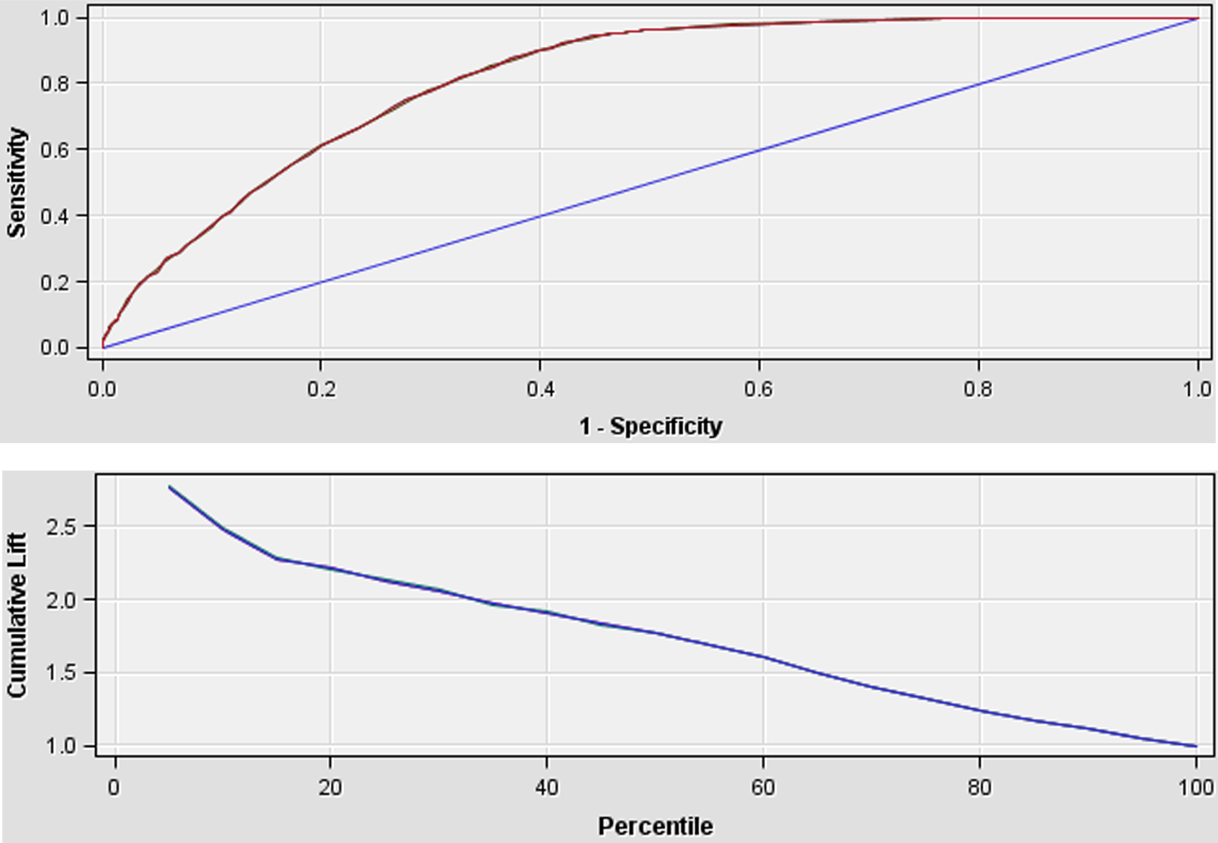
ROC curve and cumulative Lift chart of the CD model.
For the other 5 models we will content with to provide only the Gini values and the lift values at the top NP cases (Table 3). We see that, in terms of Gini, LA and CD models are the most successful but in terms of Lift at NP, IM model is the best followed by LA, DD and CD models. In our opinion Lift at NP is a more useful measure since it will show the efficiency of the model to IC operations in a more direct way.
Gini values and lift at NP cases
As the performance measures are analyzed altogether (check Tables 1 3), we can make the following observations: First of all, we have to state that the performances of all models can be expected to be better when they are applied to the full data of credits and where the samples will not be biased to high amount credits as it is now. Unfortunately, we do not have a chance to see that affect now since in the past, other credits were not inspected at all. Secondly, we observe that the performances are better for the models where we had a lot of positive cases in the past (e.g. CD, LA) and worse where there were not sufficient positive examples to learn (e.g. DQ, DD).
We want to say a few words about the performance of our models as compared to the models in the literature. But, as we have indicated before, so far there is no other study on internal control in the literature and thus, a one-to-one comparison is not possible. However, we think that our models can be listed in the risk domain and maybe the well-studied application or behavioral credit risk scoring models can be used as a benchmark to our models. Note that, application scorecards are used to decide if a loan is to be granted to a customer and behavioral scorecards are used to assess customers that have been granted credit before. Naturally, behavioral scorecards are expected to be more powerful than the application scorecards since more information would be available. As for the internal control models, we can say that, they are definitely more difficult than developing a behavior scorecard and perhaps slightly more difficult than an application scorecard since an irregularity (discrepancy, problem) cannot be directly expected from neither the information of the customer or the personnel; irregularity may appear from the combination of many factors/parties. Also, the number of minor class examples are typically less than that of application scorecard datasets.
We identified five recent papers from the literature, each of which compared a number of different classifiers for application or behavioral scorecards. The range of Gini values reported in those papers are tabulated in Table 4 where
Performance comparison with literature
Without going into detailed variable names and model equations, we can provide some ideas about what kind of information are contained in the six models as follows:
Summary and conclusions
In this study, to the best of our knowledge, we, for the first time in the literature, have undertaken developing predictive models with the aim of increasing the efficiency of a bank internal control department. Since it would not be logical to develop separate models for all scenarios being used, we have decided to group the findings of the inspections and this way we developed six models. As we analyze the performances of these models, we can see that they will bring a worthy efficiency to internal controlling with an average Gini of 51 per cent and an average lift of 3.32 when NP cases are to be inspected.
One of the limitations of this study is that we had to content with the past inspections data only. In other words, we could learn only from the previous inspections but since we did not know the result if ever some other credits were inspected, we could not use them in model development. However, since these models will be applied to the full range of credits, in the future revisions of the models we could learn from much different credit types and thus the new generation models could be more successful. Six months after their implementation, we were happy to hear verbally from the bank that, even this version of the models has already increased the performance of the inspectors by about 30 per cent. We can believe that second version models will have even better performances.
As a BPR (business process reengineering) suggestion, we can recommend the bank to group some of the similar scenarios and let them be inspected by the same inspector at once. At the current practice each scenario is inspected separately and independently, and the same credit can be seen by many inspectors. Since the bank size is very big, this might look reasonable, but we believe that our suggestion can bring some time saving since, once the personnel is concentrated on a credit, he or she can inspect several scenarios in a shorter time.
As a future work, besides developing more competitive versions of the IC models perhaps by using other classifiers also, one can try developing models for the Internal Audit department which is one of the other departments that received less attention so far. The main function of IA departments is to determine those transactions and responsible personnel that are aiming to steal money from customer accounts.
Footnotes
Acknowledgments
The author would like to Gizem Sabuncu, Buket Begüm Semercioglu and Helin Yıldırım for their contribution to discussions and helping the model development in SAS.