Blind image deconvolution via an adaptive weighted TV regularization

Abstract

Blind image deconvolution has attracted growing attention in image processing and computer vision. The total variation (TV) regularization can effectively preserve image edges. However, due to lack of self-adaptability, it does not perform very well on restoring images with complex structures. In this paper, we propose a new blind image deconvolution model using an adaptive weighted TV regularization. This model can better handle local features of image. Numerically, we design an effective alternating direction method of multipliers (ADMM) to solve this non-smooth model. Experimental results illustrate the superiority of the proposed method compared with other related blind deconvolution methods.

Keywords

Blind deconvolution Total variation regularization Adaptive weighted matrix ADMM

1 Introduction

Image deconvolution is a fundamental problem in image processing, which has attracted increasing interest in recent years. Its aim is to reconstruct a clean image from a noisy blurred image. The blurred image is usually modeled as a linear convolution of an image and a blur kernel also called the point spread function (PSF). Mathematically, the image degradation process can be described as follows: $f = k * u + η,$ (1.1) where u and f respectively represent the clean image and the degraded image, k is the blur kernel, ∗ denotes the convolution operator, and η is supposed to be an additive Gaussian white noise. There are two types, including non-blind deconvolution and blind deconvolution. When the blur kernel k is known, the problem of obtaining the clear latent image u through f and k is called non-blind deconvolution. There are a lot of research on non-blind image deconvolution [1 , 26]. However, the blur kernel is usually unknown in many practical applications. In this case, we need to estimate both u and k from f. This problem is called blind image deconvolution. In recent years, blind deconvolution has become a research hotspot in the field of image processing and computer vision [5 , 31]. Different from the non-blind deconvolution, the blind one is not only sensitive to noise, but also may yield many solutions [9]. For these reasons, blind image deconvolution is more challenging than the non-blind one [6, 12].

To solve the blind deconvolution problem, many regularization techniques have been studied. You et al. [32] proposed a blind deconvolution method by employing the H¹ norm to minimize the image u and the blur kernel k. The H¹ norm minimization problem for u and k can be expressed as $min_{k, u} \frac{1}{2} ∥ k * u - f ∥_{2}^{2} + α ∥ u ∥_{H^{1}}^{2} + β ∥ k ∥_{H^{1}}^{2},$ (1.2) where the first term is the data fidelity term, and the other two terms are the H¹ norm of u and k, respectively. α and β are two regularization parameters. However, the H¹ norm has very strong isotropic smoothing properties, which makes the method unsatisfactory on preserving the edges. In [25], Rudin et al. proposed a total variational (TV) regularization model for Gaussian image denoising. This model can better preserve edges of image while removing noise. Since then, Chan et al. [4] proposed a new blind deconvolution method by using TV regularization instead of H¹ norm: $min_{k, u} \frac{1}{2} ∥ k * u - f ∥_{2}^{2} + α ∥ \nabla u ∥_{1} + β ∥ \nabla k ∥_{1} .$ (1.3) The TV regularization performs very well on preserving edges while removing noise and blur, especially for piecewise constant images. However, due to the nonlinearity and non-differentiability of TV-based models, it is difficult to solve in calculation. Therefore, a variety of algorithms have been developed to deal with these problems [11 , 28].

Recently, blind image deconvolution has attracted growing attention in image processing [14 , 37]. Money et al. [17] applied the shock filter to pre-process the degraded image, and then used the pre-processed image as an initial condition for TV minimization blind deconvolution. This method can save the computational time, compared with the AM method in [4]. To further reduce the computational cost, the split Bregman algorithm was proposed in [15] to solve the TV blind deconvolution problem (1.3). Specifically, this method has better recovery effect on various types of blur than the proposed method in [17]. Although the TV regularization performs well on preserving edges, it is not good at keeping textures of image. Therefore, Zuo et al. [37] proposed an adaptive non-local TV method for blind image restoration. This method can fully utilize the spatial information distributed in different image regions via the non-local TV operator, and thus can preserve more details of image. Owing to the fact that cartoon and texture components can be represented differently in images, Wang et al. [27] used cartoon-texture decomposition technique for textures preservation in blind image deconvolution. Additionally, the TV norm is easy to convert the smooth signal into piecewise constant, which leads to staircase effects. To eliminate the staircase effects, Li et al. [14] proposed a non-convex high-order TV model for blind image deconvolution. However, the high-order TV regularization is not ideal for preserving image edges. In [35], Zhang et al. proposed a blind deconvolution model based on edge-preserving of L₀-regularized gradient prior. To better maintain the edges, an adaptive strategy was adopted to reduce the difficulty of parameter setting. The blur kernel estimated by this method is more accurate, which improves the performance of deblurring. In addition, many improved methods based on TV regularization were also proposed [3 , 36].

Although most of the previously studied methods can obtain relatively satisfactory results, it is not ideal to process local structures of the image. Recently, Pang et al. [21, 22] proposed some new regularization techniques combining an adaptive weighted matrix with gradient operator for image denoising. The adaptive weighted matrix can rotate the direction of the gradient operator and make it tend to a larger weight, so it can better describe the local features of image. This fact motivates us to apply this adaptive weighted TV regularization for blind deconvolution. The major contributions of the paper are three-fold:

We propose an adaptive weighted TV model for blind image deconvolution. Owing to the use of an adaptive weighted matrix, the proposed model can better deal with local structures of image.

We design an effective ADMM to solve the proposed model. The proposed algorithm may yield a unique solution.

Extensive experiments are carried out under different blur types and noise levels to show that our proposed method has better performance than other two methods for blind image deconvolution.

Fig. 1

Diagram of the basic idea for our proposed method.

The block diagram of the basic idea of our proposed method is shown in Fig 1. The rest of this paper is organized as follows. In Section 2, we first introduce some relevant preliminaries, and then propose an adaptive weighted TV blind image deconvolution model. Section 3 presents an efficient ADMM to solve the proposed model. In Section 4, we give some related experimental results to demonstrate the effectiveness and superiority of the proposed method. Finally, we end the paper with some conclusions in Section 5.

2 The proposed model

This section is devoted to presenting a new model for blind image deconvolution, where an adaptive weighted matrix is integrated with the gradient operator. Then we make a comparison with other two methods on purpose, strengths and weaknesses.

Table 1
Comparative analysis of different methods

Method Purpose Strengths Weaknesses

TV-BDSB Motion, Gaussian, Out-of-focus Uses the TV regularization to effectively preserve image edges. The algorithm is efficient. The method lacks self-adaptability.

EP-L₀RG Motion Uses an edge adaptive strategy to reduce the difficulty of parameter settings. The method estimates a more accurate kernel. It does not have universality.

AWTV-BD Motion, Gaussian, Out-of-focus Uses a novel adaptive weighted TV regularization to handle local features of image, which has a strong ability to deal with normal and simple blurred images. It is not applicable for images generated by using complex non-linear motion blur kernels.

Method	Purpose	Strengths	Weaknesses
TV-BDSB	Motion, Gaussian, Out-of-focus	Uses the TV regularization to effectively preserve image edges. The algorithm is efficient.	The method lacks self-adaptability.
EP-L₀RG	Motion	Uses an edge adaptive strategy to reduce the difficulty of parameter settings. The method estimates a more accurate kernel.	It does not have universality.
AWTV-BD	Motion, Gaussian, Out-of-focus	Uses a novel adaptive weighted TV regularization to handle local features of image, which has a strong ability to deal with normal and simple blurred images.	It is not applicable for images generated by using complex non-linear motion blur kernels.

Generally speaking, different regions of image have different structures. It is crucial to preserve local structures for the proposed model. Since the finite difference scheme of gradient only depends on the horizontal and vertical directions, traditional TV-based models cannot couple with local structures of image efficiently. To overcome this drawback, some adaptive techniques have been proposed in many image applications [20 , 29]. Specifically, in [22], the authors proposed an anisotropic TV (ATV) model for Gaussian image denoising, which can better diffuse along the tangent direction of local features. To couple with local structures more effectively, they constructed different weights by adding an adaptive weighted matrix T. The definition of T is as follows: $\begin{matrix} T (i, j) = [\begin{matrix} t_{1} (i, j) & 0 \\ 0 & t_{2} (i, j) \end{matrix}] \\ = [\begin{matrix} \frac{1}{1 + ι | G_{δ} (i, j) * \nabla_{x} f (i, j) |} & 0 \\ 0 & \frac{1}{1 + ι | G_{δ} (i, j) * \nabla_{y} f (i, j) |} \end{matrix}], \end{matrix}$ (2.1) where G_δ (·) denotes the 2D Gaussian convolution kernel, δ and ι are two tuning parameters, ∇_xf and ∇_yf represent the differences of f in the horizontal and vertical directions.

For blind image deconvolution, we consider combining the adaptive weighted matrix T with the gradient operator ∇. Besides, the L₁ norm is used to constrain ∇k. Therefore, we propose the following adaptive weighted TV model for blind image deconvolution: $min_{u, k} \frac{1}{2} ∥ k * u - f ∥_{2}^{2} + α ∥ T \nabla u ∥_{1} + β ∥ \nabla k ∥_{1},$ (2.2) where α and β are two regularization parameters used to balance the fidelity term and the regularization terms. In experiments, we also considered ∥k ∥ ₁. In most cases, we find that the blind deconvolution method using ∥ ∇ k ∥ ₁ performs better than that employing ∥k ∥ ₁. In addition, we show the comparative analysis of different methods about blind image deconvolution in Table 1.

3 Algorithm

In this section, we design an ADMM to solve the proposed model (2.2). The solution of the initial problem is transformed into alternating calculation of several simple subproblems. The ADMM has been widely used in convex and non-convex optimization, especially for the problems with non-differentiable functionals [7, 34]. It also has many applications in the field of blind image deconvolution [8 , 24].

To apply the ADMM, we introduce three auxiliary variables p, q, w to rewrite the proposed model (2.2) as a constrained optimization problem: ${\begin{matrix} min_{u, k, p, q, w} \frac{1}{2} ∥ k * u - f ∥_{2}^{2} + α ∥ q ∥_{1} + β ∥ w ∥_{1}, \\ s . t . p = \nabla u, q = Tp, w = \nabla k . \end{matrix}$ (3.1) To solve (3.1), three Lagrangian multipliers λ₁, λ₂, λ₃ are introduced to reformulate it as a saddle point problem, whose augmented Lagrangian functional is $\begin{matrix} L (k, u, p, q, w; λ_{1}, λ_{2}, λ_{3}) = \frac{1}{2} ∥ Ku - f ∥_{2}^{2} \\ + α ∥ q ∥_{1} + β ∥ w ∥_{1} + \frac{r_{1}}{2} ∥ p - \nabla u - λ_{1} ∥_{2}^{2} \\ + \frac{r_{2}}{2} ∥ q - Tp - λ_{2} ∥_{2}^{2} + \frac{r_{3}}{2} ∥ w - \nabla k - λ_{3} ∥_{2}^{2} . \end{matrix}$ (3.2) Here, K represents the unknown blurring matrix which is a block-circulant matrix formed by the point spread function k. r₁, r₂ and r₃ are three penalty parameters. While applying the ADMM, we need to minimize five subproblems and update three Lagrangian multipliers with other variables fixed at each iteration. Namely, we have ${\begin{matrix} k^{n + 1} = arg min_{k} L (k, u^{n}, p^{n}, q^{n}, w^{n}; λ_{1}^{n}, λ_{2}^{n}, λ_{3}^{n}), \\ u^{n + 1} = arg min_{u} L (k^{n + 1}, u, p^{n}, q^{n}, w^{n}; λ_{1}^{n}, λ_{2}^{n}, λ_{3}^{n}), \\ p^{n + 1} = arg min_{p} L (k^{n + 1}, u^{n + 1}, p, q^{n}, w^{n}; λ_{1}^{n}, λ_{2}^{n}, λ_{3}^{n}), \\ q^{n + 1} = arg min_{q} L (k^{n + 1}, u^{n + 1}, p^{n + 1}, q, w^{n}; λ_{1}^{n}, λ_{2}^{n}, λ_{3}^{n}), \\ w^{n + 1} = arg min_{w} L (k^{n + 1}, u^{n + 1}, p^{n + 1}, q^{n + 1}, w; λ_{1}^{n}, λ_{2}^{n}, λ_{3}^{n}), \\ λ_{1}^{n + 1} = λ_{1}^{n} + \nabla u^{n + 1} - p^{n + 1}, \\ λ_{2}^{n + 1} = λ_{2}^{n} + {Tp}^{n + 1} - q^{n + 1}, \\ λ_{3}^{n + 1} = λ_{3}^{n} + \nabla k^{n + 1} - w^{n + 1} . \end{matrix}$ (3.3) In the following, we give explicit solutions of the above subproblems.

The k-subproblem can be expressed as $k^{n + 1} = arg min_{k} \frac{1}{2} ∥ U^{n} k - f ∥_{2}^{2} + \frac{r_{3}}{2} ∥ w^{n} - \nabla k - λ_{3}^{n} ∥_{2}^{2},$ (3.4) where U is a block-circulant matrix which is formed by the image u. According to the optimality conditions, it is easy to derive the Euler-Lagrange equation of (3.4). In this paper, we assume periodic boundary condition. And hence, this equation can be solved efficiently by the fast Fourier transform (FFT). In this way, we can get $k^{n + 1} = F^{- 1} [\frac{F ((U^{n})^{T} f + r_{3} \nabla^{T} (w^{n} - λ_{3}^{n}))}{F ((U^{n})^{T} U^{n} + r_{3} \nabla^{T} \nabla)}],$ (3.5) where F denotes the FFT and $\overset{- 1}{F}$ represents its inverse transform. ∇^T means the conjugate transpose of the gradient operator ∇.

The u-subproblem can be written as $u^{n + 1} = arg min_{u} \frac{1}{2} ∥ K^{n + 1} u - f ∥_{2}^{2} + \frac{r_{1}}{2} ∥ p^{n} - \nabla u - λ_{1}^{n} ∥_{2}^{2} .$ (3.6) Similarly, considering its optimality conditions and then using the FFT, we have $u^{n + 1} = F^{- 1} [\frac{F ((K^{n + 1})^{T} f + r_{1} \nabla^{T} (p^{n} - λ_{1}^{n}))}{F ((K^{n + 1})^{T} K^{n + 1} + r_{1} \nabla^{T} \nabla)}] .$ (3.7) For the p-subproblem, it can be expressed as $\begin{matrix} p^{n + 1} & = arg min_{p} \frac{r_{1}}{2} ∥ p - \nabla u^{n + 1} - λ_{1}^{n} ∥_{2}^{2} \\ + \frac{r_{2}}{2} ∥ q^{n} - T p - λ_{2}^{n} ∥_{2}^{2} . \end{matrix}$ (3.8) We also consider its optimality conditions. Denote p = [p₁, p₂] , q = [q₁, q₂] , λ_i = [λ_i1, λ_i2] (i = 1, 2). Then the corresponding linear equation can be arranged as $\begin{matrix} [\begin{matrix} r_{1} + r_{2} t_{1}^{2} & 0 \\ 0 & r_{1} + r_{2} t_{2}^{2} \end{matrix}] [\begin{matrix} p_{1}^{n + 1} \\ p_{2}^{n + 1} \end{matrix}] = \\ [\begin{matrix} r_{1} (\nabla_{x} u^{n + 1} + λ_{11}^{n}) + r_{2} t_{1} (q_{1}^{n} - λ_{21}^{n}) \\ r_{1} (\nabla_{y} u^{n + 1} + λ_{12}^{n}) + r_{2} t_{2} (q_{2}^{n} - λ_{22}^{n}) \end{matrix}] . \end{matrix}$ (3.9) Obviously, the subproblem (3.8) is a smooth optimization problem. Thus, we can obtain the explicit solution of pⁿ⁺¹ from the linear equation system (3.9) through a simple calculation, ${\begin{matrix} p_{1}^{n + 1} = \frac{r_{1} (\nabla_{x} u^{n + 1} + λ_{11}^{n}) + r_{2} t_{1} (q_{1}^{n} - λ_{21}^{n})}{r_{1} + r_{2} t_{1}^{2}}, \\ p_{2}^{n + 1} = \frac{r_{1} (\nabla_{y} u^{n + 1} + λ_{12}^{n}) + r_{2} t_{2} (q_{2}^{n} - λ_{22}^{n})}{r_{1} + r_{2} t_{2}^{2}} . \end{matrix}$ (3.10)

For the q-subproblem, it can be written as $q^{n + 1} = arg min_{q} α ∥ q ∥_{1} + \frac{r_{2}}{2} ∥ q - T p^{n + 1} - λ_{2}^{n} ∥_{2}^{2},$ (3.11) which has a closed form solution. And its solution can be given by the extremely fast shrinkage formula $q_{i, j}^{n + 1} = shrinkage ((T p^{n + 1} + λ_{2}^{n})_{i, j} \frac{α}{r_{2}}) .$ (3.12)

The w-subproblem can be expressed as $w^{n + 1} = arg min_{w} β ∥ w ∥_{1} + \frac{r_{3}}{2} ∥ w - \nabla k^{n + 1} - λ_{3}^{n} ∥_{2}^{2} .$ (3.13) Similar to the q-subproblem, the solution of the w-subproblem can be given by the extremely fast shrinkage formula $w_{i, j}^{n + 1} = shrinkage ((\nabla k^{n + 1} + λ_{3}^{n})_{i, j} \frac{β}{r_{3}}) .$ (3.14)

We note that the solution (k, u) of the proposed model (2.2) is not unique. Hence some constraints on k and u are needed to impose so as to obtain a unique reasonable solution. Similar to the previous blind deconvolution methods [4, 15], we normalize the estimated PSF and consider the non-negativity of image intensity during the iterative process. Namely, we utilize $\int k^{n} (x, y) dxdy = 1,$ (3.15) and $u^{n} (x, y) = {\begin{matrix} u^{n} (x, y), u^{n} (x, y) \geq 0, \\ 0, else . \end{matrix}$ (3.16) Besides, to reduce the effect of noise which exists in the estimated PSF, we refine the PSF using a dynamic threshold constraint. In this paper, we use $k^{n} (x, y) = {\begin{matrix} k^{n} (x, y), k^{n} (x, y) \geq ξ max (k^{n}), \\ 0, else, \end{matrix}$ (3.17) where max(kⁿ) represents the maximum value of the nth estimated PSF, and ξ is a small positive constant. Specifically, we set ξ=0.05 in our experiments.

The whole algorithm for solving the proposed model (2.2) is summarized in Algorithm 3.1.

Algorithm 3.1. (ADMM for solving (2.2))

Step 1. Input and initialization: $u^{0} = f, p^{0} = λ_{1}^{0} = q^{0} = λ_{2}^{0} = w^{0} = λ_{3}^{0} = 0$ . Let n : =0.

Step 2. Compute kⁿ⁺¹ by (3.5).

Step 3. Impose constraints on kⁿ⁺¹ by (3.15) and (3.17).

Step 4. Compute uⁿ⁺¹ by (3.7).

Step 5. Impose constraint on uⁿ⁺¹ by (3.16).

Step 6. Compute pⁿ⁺¹ by (3.10).

Step 7. Compute qⁿ⁺¹ by (3.12).

Step 8. Compute wⁿ⁺¹ by (3.14).

Step 9. Update $(λ_{1}^{n + 1}, λ_{2}^{n + 1}, λ_{3}^{n + 1})$ by the last three equations of (3.3).

Step 10. Stop if the stopping criterion is satisfied. Otherwise, let n : = n + 1 and go to Step 2.

Fig. 2

Test images.

Fig. 3

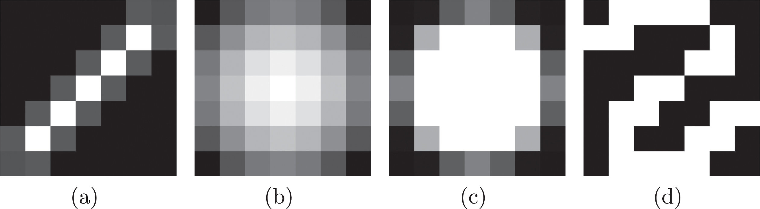
Blur kernels for image degradation: (a) linear motion, (b) Gaussian, (c) out-of-focus, (d) customized.

Table 2

Selected parameter sets for different models under different blur types and noise levels

Image	Blur type	Noise	TV-BDSB	EP-L₀RG	AWTV-BD
			(α,β)	(β₁,β₂,λ₁)	(α,β,ι,δ)
Satellite (256×256)	Linear motion	0.001	(0.00006,0.1)	(1,0.4,0.001)	(0.00005,0.1,25,1)
	Gaussian		(0.000005,0.06)	(0.85,0.63,0.0025)	(0.000005,0.05,15,1)
	Out-of-focus		(0.000006,0.03)	(0.8,0.55,0.002)	(0.000007,0.02,15,1)
	Customized		(0.0001,0.05)	(0.9,0.5,0.0035)	(0.00006,0.002,35,1)
Lena (256×256)	Linear motion	0.001	(0.00007,0.008)	(1.1,0.7,0.004)	(0.00005,0.001,90,0.6)
	Gaussian		(0.00002,0.02)	(0.9,0.8,0.0023)	(0.00002,0.02,90,1)
	Out-of-focus		(0.00002,0.05)	(0.85,0.5,0.0055)	(0.00002,0.05,60,1)
	Customized		(0.00015,0.0001)	(0.7,0.6,0.003)	(0.00009,0.0004,50,1)
Peppers (256×256)	Linear motion	0.001	(0.0002,0.7)	(0.9,0.5,0.0043)	(0.0001,0.6,10,1)
	Gaussian		(0.00008,1.1)	(0.65,0.7,0.0036)	(0.00006,1.1,40,1)
	Out-of-focus		(0.000023,0.05)	(0.8,0.67,0.001)	(0.000022,0.09,50,1)
	Customized		(0.0013,0.5)	(1,0.5,0.003)	(0.0006,0.1,150,1)
	Linear motion	0.01	(0.0009,0.04)	(0.8,0.3,0.004)	(0.001,0.007,100,1)
	Gaussian		(0.0006,1.9)	(0.4,0.5,0.0023)	(0.0007,1.4,400,1)
	Out-of-focus		(0.0005,0.9)	(0.8,0.4,0.0013)	(0.0006,0.8,70,1)
	Customized		(0.0013,1.6)	(1,0.7,0.003)	(0.0014,1.3,90,1)
House (256×256)	Linear motion	0.001	(0.00046,0.69)	(1,0.6,0.0015)	(0.00035,0.7,20,1)
	Gaussian		(0.0001,1.1)	(0.8,0.75,0.005)	(0.00008,0.9,30,1)
	Out-of-focus		(0.00015,0.13)	(0.9,1,0.003)	(0.00009,0.44,130,1)
	Customized		(0.004,1.7)	(0.85,0.7,0.0024)	(0.002,0.7,230,1)
	Linear motion	0.01	(0.0011,0.01)	(1,0.7,0.001)	(0.0014,0.08,150,1)
	Gaussian		(0.0009,0.7)	(0.9,0.6,0.0044)	(0.0008,1,250,1)
	Out-of-focus		(0.0006,0.6)	(1,0.55,0.002)	(0.0005,0.5,130,1)
	Customized		(0.002,5)	(1.1,0.4,0.0013)	(0.003,3,250,1)

4 Numerical experiments

In this section, comprehensive experimental results for our proposed method are presented to illustrate the effectiveness and superiority over other related blind deconvolution methods: TV-BDSB [15] and EP-L₀RG [35]. For simplicity of presentation, we denote the newly developed method as AWTV-BD. All the numerical experiments are conducted in MATLAB environment on a PC with 3.20GHz AMD Ryzen 7 5800H CPU and 16GB RAM. We use the peak signal-to-noise ratio (PSNR), the improved signal-to-noise ratio (ISNR) and the structural similarity (SSIM) as quantitative indexes to evaluate the quality of restoration results. Their definitions are expressed as $PSNR = 10 {log}_{10} \frac{1^{2}}{\frac{1}{MN} \sum_{i = 1}^{M} \sum_{j = 1}^{N} (u_{i, j} - I_{i, j})^{2}},$ (4.1) $ISNR = 10 {log}_{10} \frac{∥ f - I ∥_{2}^{2}}{∥ u - I ∥_{2}^{2}},$ (4.2) $SSIM = \frac{(2 μ_{I} μ_{u} + c_{1}) (2 σ_{Iu} + c_{2})}{({μ_{I}}^{2} + {μ_{u}}^{2} + c_{1}) ({σ_{I}}^{2} + {σ_{u}}^{2} + c_{2})},$ (4.3) where f, I and u denote the degraded, original and restored images, respectively. M and N are the length and width of an image. μ and σ represent the local mean value and the standard deviation of image, respectively. σ_Iu is the covariance value between I and u. c₁ and c₂ are two constants used to avoid near-zero denominator values. Generally, the higher the values of PSNR, ISNR and SSIM, the better the quality of the restored image. The definition of the relative error of solution $\overset{n}{u}$ is $R (u^{n}) = \frac{∥ u^{n} - u^{n - 1} ∥_{2}}{∥ u^{n - 1} ∥_{2}} .$ (4.4) The iteration will terminate when R (uⁿ) <10^-4 or the iteration reaches 500 in all experiments.

Table 3

Numerical results for blind deconvolution under Gaussian noise with standard variance of 0.001

Image	Blur type	Method	PSNR	ISNR	SSIM
Satellite	Linear motion	TV-BDSB	40.17	14.20	0.993
		EP-L₀RG	33.04	7.08	0.974
		AWTV-BD	40.30	14.34	0.992
	Gaussian	TV-BDSB	35.99	11.77	0.947
		EP-L₀RG	30.30	6.08	0.956
		AWTV-BD	36.08	11.87	0.947
	Out-of-focus	TV-BDSB	38.65	13.37	0.964
		EP-L₀RG	32.03	6.75	0.969
		AWTV-BD	38.75	13.47	0.964
Peppers	Linear motion	TV-BDSB	32.64	9.16	0.941
		EP-L₀RG	27.96	4.48	0.872
		AWTV-BD	33.38	9.90	0.947
	Gaussian	TV-BDSB	33.39	10.89	0.938
		EP-L₀RG	26.36	3.86	0.822
		AWTV-BD	33.56	11.06	0.940
	Out-of-focus	TV-BDSB	34.34	10.68	0.950
		EP-L₀RG	29.21	5.56	0.875
		AWTV-BD	35.32	11.66	0.955
Lena	Linear motion	TV-BDSB	33.18	7.97	0.944
		EP-L₀RG	30.28	5.07	0.881
		AWTV-BD	33.46	8.25	0.947
	Gaussian	TV-BDSB	32.90	9.38	0.924
		EP-L₀RG	29.14	5.62	0.855
		AWTV-BD	33.20	9.68	0.927
	Out-of-focus	TV-BDSB	34.91	9.95	0.941
		EP-L₀RG	30.12	5.16	0.859
		AWTV-BD	35.18	10.22	0.943
House	Linear motion	TV-BDSB	33.60	8.94	0.928
		EP-L₀RG	30.04	5.38	0.871
		AWTV-BD	34.38	9.72	0.934
	Gaussian	TV-BDSB	36.00	12.37	0.930
		EP-L₀RG	28.77	5.14	0.843
		AWTV-BD	36.18	12.55	0.932
	Out-of-focus	TV-BDSB	34.50	9.08	0.931
		EP-L₀RG	29.62	4.21	0.858
		AWTV-BD	35.78	10.37	0.940

Table 4

Numerical results for customized blur under Gaussian noise with standard variance of 0.001

Image	Blur type	Method	PSNR	ISNR	SSIM
Satellite	Customized	TV-BDSB	43.71	19.43	0.996
		EP-L₀RG	32.34	8.06	0.974
		AWTV-BD	45.19	20.91	0.993
Peppers	Customized	TV-BDSB	29.01	6.62	0.875
		EP-L₀RG	32.17	9.78	0.916
		AWTV-BD	31.09	8.70	0.919
Lena	Customized	TV-BDSB	35.05	11.23	0.951
		EP-L₀RG	31.76	7.94	0.898
		AWTV-BD	35.57	11.75	0.957
House	Customized	TV-BDSB	29.50	6.06	0.857
		EP-L₀RG	30.55	7.11	0.870
		AWTV-BD	32.43	8.98	0.884

Fig. 4

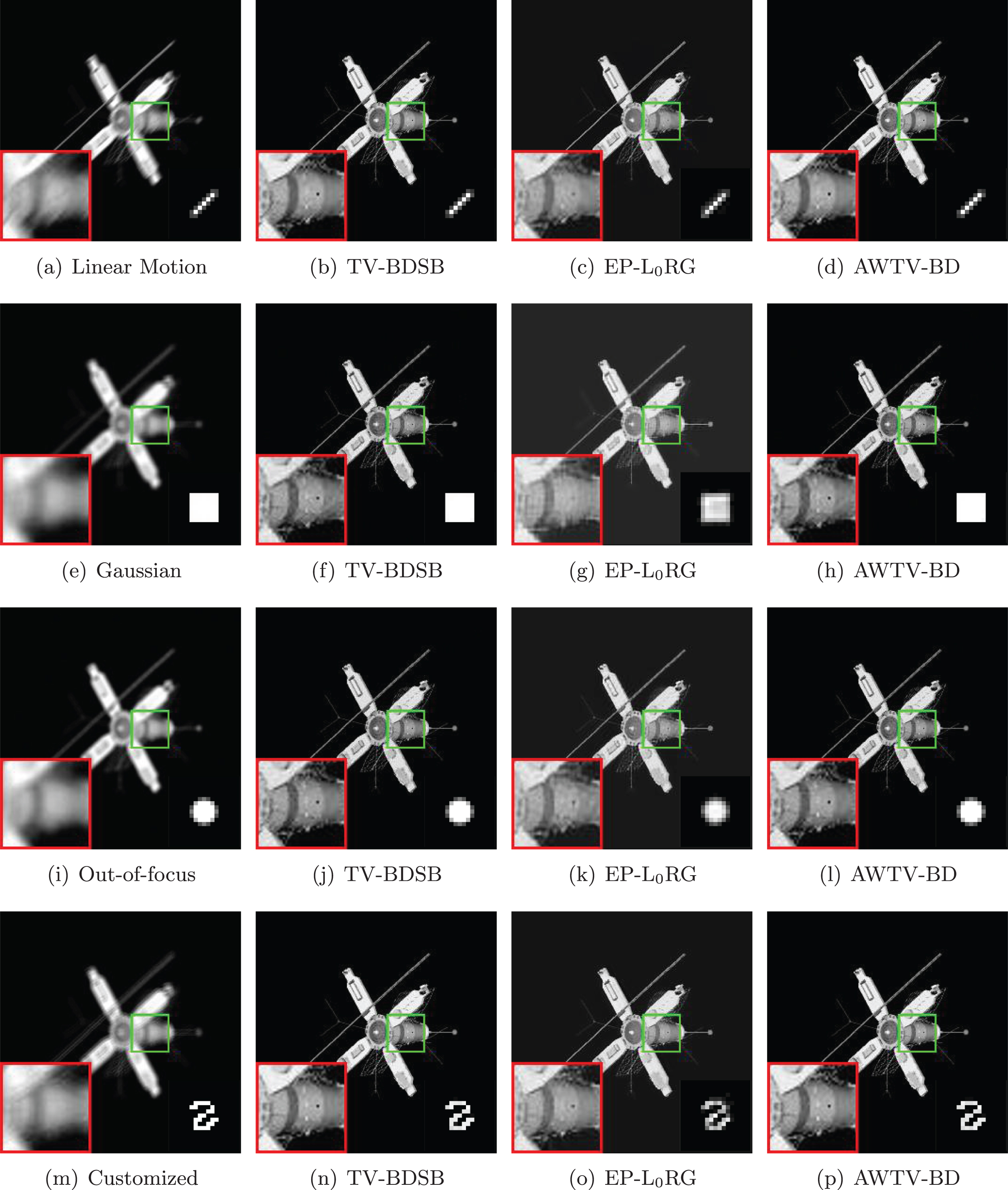
Blind deconvolution results of the Satellite image obtained by different methods under noise level 0.001.

Fig. 5

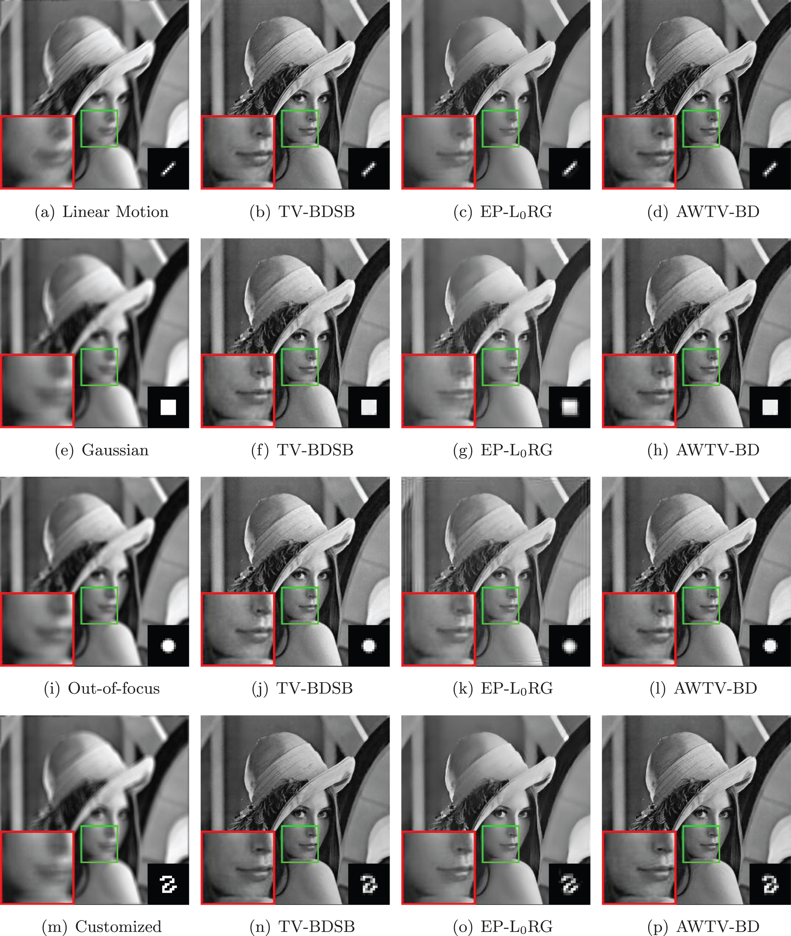
Blind deconvolution results of the Lena image obtained by different methods under noise level 0.001.

In experiments, there are four test images including Satellite (256 × 256), Peppers (256 × 256), Lena (256 × 256) and House (256 × 256) [7 , 33], as shown in Fig 1. The intensities of these images are first scaled into the range between 0 and 1. To obtain degraded images, the Matlab command “fspecial" is used to generate three different blur kernels, including linear motion blur (length of 8 pixels and direction of 45 degree), Gaussian blur (size of 7 × 7 pixels, variance of 25) and out-of-focus blur (radius of 3 pixels). The last customized blur is a simulated irregular motion blur, which is manually set to ([0 1 1 1 1 0 0; 1 1 0 0 0 1 0; 0 0 0 0 1 1 0; 0 0 1 1 0 0 0; 0 1 1 0 0 1 1; 0 1 0 0 1 1 0; 0 1 1 1 1 0 0]/22). The blur kernels we used are presented in Fig. 2.

4.1 Parameters discussion

Before the proposed algorithm is executed, we need to set seven parameters manually, i.e., α, β, ι, δ, r₁, r₂ and r₃. α controls the weight of the image regularization term. If α is too large, it will cause the restored image too smooth and lose some details of the image. On the contrary, if α is too small, the noise will not be removed well. In short, the selection of α is usually related to the degree of noise pollution of the image. When the initial clean image is polluted by high noise, the larger α should be selected. In experiments, we set α ∈ [0.000001, 0.01]. β is a regularization parameter for blur kernel k, which affects the spread of the PSF. If β is excess big, the estimated PSF will have more diffuse. Conversely, the support domain of the estimated PSF will not be fully expanded. We set β ∈ [0.0001, 10] in experiments. To obtain satisfactory deconvolution results, it is crucial to choose appropriate values for these two parameters.

ι is a tuning parameter used to control the local adaptivity, and δ is the standard deviation. In the process of parameter adjustment, we observe that the selection of ι will be affected by the test images and blur types. Therefore, we need to adjust according to specific experiment. In addition, we can find that δ has little influence on the PSNR value of the restored image.

r₁, r₂ and r₃ are three penalty parameters. According to equations (3.10), (3.12) and (3.14), they control the update of p, q and w. Empirically, we set r₁ ∈ [0.00001, 10], r₂ ∈ [0.000001, 1]. To obtain the highest PSNR value, we set the value of r₃ to multiple of 5 in most cases. In addition, Table 2 lists the optimal values of related parameters used for numerical comparison of different methods.

4.2 Blind deconvolution

Table 5
Numerical results for blind deconvolution under Gaussian noise with standard variance of 0.01

Image Blur type Method PSNR ISNR SSIM

Peppers Linear motion TV-BDSB 27.35 3.96 0.855

EP-L₀RG 26.37 2.98 0.841

AWTV-BD 28.22 4.83 0.871

Gaussian TV-BDSB 28.76 6.34 0.841

EP-L₀RG 25.86 3.43 0.812

AWTV-BD 29.33 6.90 0.863

Out-of-focus TV-BDSB 26.87 3.31 0.838

EP-L₀RG 26.12 2.56 0.832

AWTV-BD 28.37 4.82 0.861

Customized TV-BDSB 28.49 6.18 0.858

EP-L₀RG 29.12 6.80 0.852

AWTV-BD 28.94 6.63 0.865

House Linear motion TV-BDSB 30.28 5.73 0.883

EP-L₀RG 29.61 5.06 0.859

AWTV-BD 31.70 7.15 0.893

Gaussian TV-BDSB 31.44 7.91 0.872

EP-L₀RG 28.64 5.11 0.836

AWTV-BD 32.21 8.68 0.875

Out-of-focus TV-BDSB 30.33 5.07 0.868

EP-L₀RG 28.98 3.72 0.847

AWTV-BD 31.89 6.63 0.874

Customized TV-BDSB 29.53 6.18 0.847

EP-L₀RG 30.05 6.69 0.859

AWTV-BD 31.09 7.73 0.867

Image	Blur type	Method	PSNR	ISNR	SSIM
Peppers	Linear motion	TV-BDSB	27.35	3.96	0.855
		EP-L₀RG	26.37	2.98	0.841
		AWTV-BD	28.22	4.83	0.871
	Gaussian	TV-BDSB	28.76	6.34	0.841
		EP-L₀RG	25.86	3.43	0.812
		AWTV-BD	29.33	6.90	0.863
	Out-of-focus	TV-BDSB	26.87	3.31	0.838
		EP-L₀RG	26.12	2.56	0.832
		AWTV-BD	28.37	4.82	0.861
	Customized	TV-BDSB	28.49	6.18	0.858
		EP-L₀RG	29.12	6.80	0.852
		AWTV-BD	28.94	6.63	0.865
House	Linear motion	TV-BDSB	30.28	5.73	0.883
		EP-L₀RG	29.61	5.06	0.859
		AWTV-BD	31.70	7.15	0.893
	Gaussian	TV-BDSB	31.44	7.91	0.872
		EP-L₀RG	28.64	5.11	0.836
		AWTV-BD	32.21	8.68	0.875
	Out-of-focus	TV-BDSB	30.33	5.07	0.868
		EP-L₀RG	28.98	3.72	0.847
		AWTV-BD	31.89	6.63	0.874
	Customized	TV-BDSB	29.53	6.18	0.847
		EP-L₀RG	30.05	6.69	0.859
		AWTV-BD	31.09	7.73	0.867

Table 6

The computational time of each blind deconvolution method under Gaussian blur and noise level 0.01

Method	TV-BDSB	EP-L₀RG	AWTV-BD
Image	CPU	CPU	CPU
Peppers (256×256)	24.359	65.597	29.531
Peppers (512×512)	65.546	122.257	82.765
House (256×256)	16.421	60.543	22.735
House (512×512)	52.265	115.245	66.536

Fig. 6

Blind deconvolution results of the Peppers image under noise level 0.01.

Fig. 7

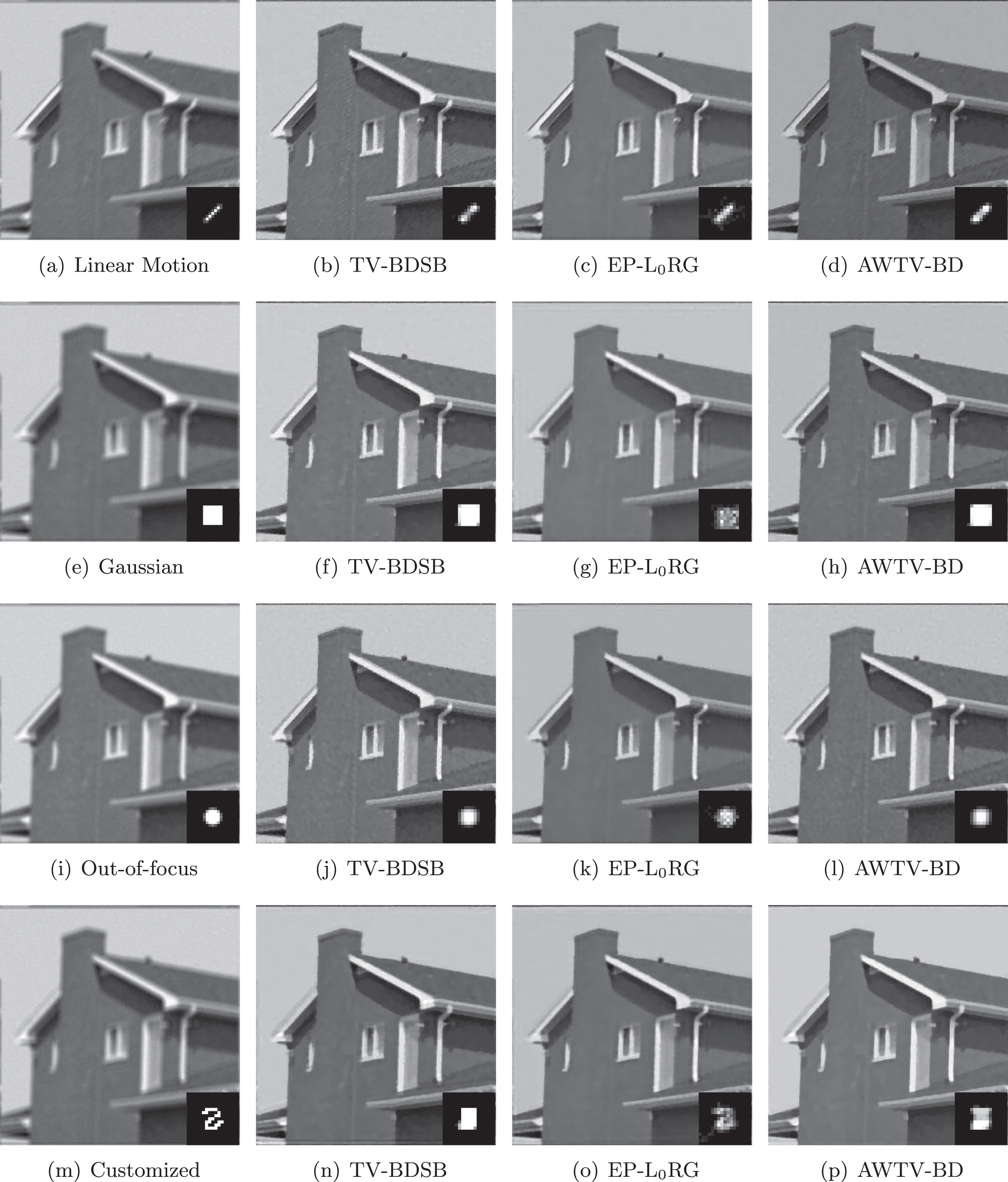
Blind deconvolution results of the House image under noise level 0.01.

Firstly, we test the blind deconvolution performance of AWTV-BD at low noise level. The blurred images generated by adding four different blur kernels in Fig. 2 to the test images are polluted by additive white Gaussian noise with standard variance of 0.001. For blind image deconvolution, we require to set the support of PSF. As the true support of PSF is unknown, the size of the initial support of PSF should be larger than that of the true one, but smaller than the size of the image. In experiments, we set the size of PSF support as 101×101 pixels. The related numerical results of three methods for linear motion blur, Gaussian blur and out-of-focus blur are listed in Table 1, while displaying the results for customized blur in Table 2. From these two tables, we can see that our proposed AWTV-BD obtains the highest PSNR, ISNR and SSIM values in most cases, compared with other methods. Especially for linear motion blur, Gaussian blur and out-of-focus blur, the PSNR and ISNR values of AWTV-BD are always the highest, which can be easily seen from Table 1.

Fig. 8

Non-blind deconvolution results of different methods on two images (“Peppers", “Lena") with noise level 0.01: the restored images (row 1, 3) and the locally enlarged images (row 2, 4).

To visually evaluate the results of different methods, the restored Satellite and Lena images with the selected locally enlarged images placing in the lower left corner are shown in Fig. 3 and Fig. 4, respectively. Furthermore, the restored blur kernels are placed in the lower right corner of the images.

From the enlarged images of Fig 3, we observe that the images restored by EP-L₀RG lose a lot of details and it can not get a satisfactory visual effect. Its restored blur kernels are great difference from the original one. Fortunately, the blur kernel recovered by AWTV-BD is the closest to the original blur kernel compared with the other two methods. From the enlarged images of Fig. 4, it is easy to see that the images restored by EP-L₀RG are too smooth, which result in the loss of some details of the original image. In addition, some images obtained by TV-BDSB have obvious staircase effects in flat regions. Owing to the use of the adaptive weighted matrix, our AWTV-BD can better preserve local structures of image, especially for the face and the mouth. From the restored blur kernels, we find that AWTV-BD also produces the closest to the original blur kernel.

Further, we explore higher noise level case, say standard variance of 0.01 for the Peppers image and the House image. The blur kernels used for image blur are the same as in previous experiments. The corresponding numerical results are arranged in Table 3. Table 3 shows that AWTV-BD still achieves the highest PSNR, ISNR and SSIM values in most cases. To assess the recovery results from the visual effect, we show the restored Peppers and House images with the recovery blur kernels placing in the lower right corner in Fig. 5 and Fig. 6, respectively. From Fig. 5, we can observe that the restored images obtained by EP-L₀RG are also too smooth under high noise level, although for the customized blur, its restored blur kernel is closer to the original one. From Fig. 6, the over-smoothing effect generated by EP-L₀RG is very obvious. Our proposed AWTV-BD can overcome this problem. Besides, these two figures show that AWTV-BD produces more natural restoration images compared with other two methods. In addition, Table 6 shows the computational time for restoring the Peppers image and the House image with two sizes. We observe that the CPU time grows fast when the image size becomes larger. Moreover, our proposed method is faster than the EP-L₀RG.

4.3 Non-blind deconvolution

In this subsection, we show some results for non-blind deconvolution in which the PSF is exactly known. The non-blind deconvolution problem corresponding to model (2.2) is expressed as

min_{u} \frac{1}{2} ∥ Ku - f ∥_{2}^{2} + α ∥ T \nabla u ∥_{1} .

(4.5) Similarly, the variant of TV-BDSB for non-blind deconvolution is as follows:

min_{u} \frac{1}{2} ∥ Ku - f ∥_{2}^{2} + α ∥ \nabla u ∥_{1} .

(4.6)

Table 7

Comparison of non-blind deconvolution methods under Gaussian noise with standard deviation of 0.01

Method	TV-NBD		AWTV-NBD
Image	PSNR	SSIM	PSNR	SSIM
Satellite	33.35	0.924	33.37	0.924
Peppers	30.57	0.880	31.21	0.886
Lena	30.07	0.855	30.21	0.862
House	32.85	0.887	33.60	0.894

These two models are solved by ADMM and the split Bregman method, respectively. For convenience, we denote them as AWTV-NBD and TV-NBD. In experiments, the original images are blurred by the customized blur kernel. We add additive white Gaussian noise with standard deviation of 0.01 to the blurred images. The related numerical results are presented in Table 4. Especially, Fig. 7 shows the restored Peppers and Lena images and the selected locally enlarged images at noise level 0.01, where the first column represents the degraded images. It is easy to see from Table 4 that AWTV-NBD obtains higher PSNR and SSIM values compared with TV-NBD. From the enlarged images of Fig. 7, we observe that the restored images by AWTV-NBD are more natural owing to the use of the adaptive weighted matrix.

5 Conclusion and future work

In this paper, we proposed an adaptive weighted total variation regularization for blind image deconvolution. To better describe the local structures of image, we combined an adaptive weighted matrix with the gradient operator. Furthermore, an efficient ADMM was applied to solve the proposed model. Our proposed method can recover multiple blur types. Experiments were conducted to demonstrate the superior performance of the proposed method, especially for images degraded by linear motion blur, Gaussian blur and out-of-focus blur. For some images generated by using complex non-linear motion blur kernel such as the customized blur, our blind deconvolution method sometimes cannot get satisfactory results. This is also the part that we need to improve in the future work.

In the future, we would like to explore some acceleration techniques to further reduce the computational cost. Besides, we will focus on extending the adaptive strategy to other image processing problems, e.g., image segmentation, hyperspectral image super-resolution and hyperspectral unmixing.

Data Availability

The data used to support the findings of this study are available from the corresponding author upon request.

Competing Interests

The authors declare that they have no competing interests.

Conflict of Interest

The authors declare that they have no conflict of interest.

Acknowledgments

This work was partly supported by the Natural Science Foundation of Jiangxi Province (20192BAB211005), the Science Foundation for Post Doctorate of China (2020M672484), and the NNSF of China (61865012).

References

Adam

, Paramesran

, Hybrid non-convex second-order total variation with applications to non-blind image deblurring. Signal, Image and Video Processing. 2020;14(1):115–23.

Anger

, Facciolo

, Delbracio

Modeling realistic degradations in non-blind deconvolution. IEEE International Conference on Image Processing (ICIP), 2018;2018:978–82.

Bai

, Cheung

, Liu

, Gao

Graph-based blind image deblurring from a single photograph, IEEE Transactions on Image Processing 2018;28(3):1404–1.

Chan

, Wong

Total variation blind deconvolution. IEEE Transactions on Image Processing, 1998;7(3):370–5.

El Mourabit

, El Rhabi

, Hakim

Blind deconvolution using bilateral total variation regularization: A theoretical study and application. Applicable Analysis 2021;2021:1–14.

Gong

, Tan

, Zhang

, Hengel

, Shi

Blind image deconvolution by automatic gradient activation. Proceedings of the IEEE Conference on Computer Vision and Pattern Recognition, 2016;2016:1827–36.

Guo

, Chen

Image denoising based on nonconvex anisotropic total-variation regularization. Signal Processing, 2021;186:108124.

Han

, Kan

Blind image deblurring based on local edges selection. Applied Sciences 2019;9(16):3274.

, Marquina

, Osher

Blind deconvolution using TV regularization and Bregman iteration. International Journal of Imaging Systems and Technology 2005;15(1):74–83.

10.

Javaran

, Hassanpour

, Abolghasemi

Non-blind image deconvolution using a regularization based on re-blurring process. Computer Vision and Image Understanding 2017;154:16–34.

11.

Jin

, Grama

, Liu

Controlled total variation regularization for image deconvolution. The Imaging Science Journal 2016;64(2):68–81.

12.

Krishnan

, Tay

, Fergus

Blind deconvolution using a normalized sparsity measure. CVPR 2011;2011:233–40.

13.

, Lv

, Deng

Regularized iterative Weiner filter method for blind image deconvolution. Journal of Computational and Applied Mathematics, 2018;336:425–38.

14.

, Chen

, Xu

, Gong

Blind motion image deblurring using nonconvex higher-order total variation model. Journal of Electronic Imaging 2016;25(5):053033.

15.

, Li

, Gong

, Tang

Total variation blind deconvolution employing split Bregman iteration. Journal of Visual Communication and Image Representation 2012;23(3):409–17.

16.

, Zhang

Non-blind image deblurring method using shear high order total variation norm. JWuhan University Journal of Natural Sciences, 2021;26:495–506.

17.

Money

, Kang

Total variation minimizing blind deconvolution with shock filter reference. Image and Vision Computing 2008;26(2)302–14.

18.

Mousavi

, Mokhtari

, Lakestani

Blind deconvolution using shearlet-tv regularization. TWMS Journal of Applied and Engineering Mathematics 2019;9(3):525–34.

19.

Oliveira

, Bioucas-Dias

, Figueiredo

MAT

Adaptive total variation image deblurring: A majorization-minimization approach. Signal Processing 2009;89(9):1683–93.

20.

Pang

, Meng

, Li

, Chen

Image restoration via the adaptive TVp regularization. Computers and Mathematics with Applications 2020;80(5):569–87.

21.

Pang

, Zhang

, Luo

, Zeng

Image denoising based on the adaptive weighted TVp regularization. Signal Processing 2020;167:107325.

22.

Pang

, Zhou

, Wu

, Li

Image denoising via a new anisotropic total-variation-based model. Signal Processing: Image Communication, 2019;74:140–52.

23.

Perrone

, Favaro

Total variation blind deconvolution: The devil is in the details. Proceedings of the IEEE Conference on Computer Vision and Pattern Recognition 2014;2014:2909–16.

24.

Qian

, Wang

Spatially adaptive sparse representation prior for blind image restoration. Optik 2020;207:163893.

25.

Rudin

, Osher

, Fatemi

Non-linear total variation based noise removal algorithms. Physica D: Nonlinear Phenomena 1992;60(1-4):259–68.

26.

Tang

, Gong

, Li

, Wang

Non-blind image deblurring method by local and nonlocal total variation models. Signal Processing 2014;94:339–49.

27.

Wang

, Zhao

, Ng

A cartoon-plus-texture image decomposition model for blind deconvolution. Multidimensional Systems and Signal Processing 2016;27(2):541–62.

28.

Wang

, Yin

, Zhang

Afast algorithm for image deblurring with total variation regularization. CAAM Technical Reports TR07-10. 2007.

29.

Wen

, Sun

, Guo

A new anisotropic fourth-order diffusion equation model based on image features for image denoising. Inverse Problems and Imaging 2022;16(4):895–924.

30.

Xue

Blind image deblurring: A review. arXiv preprint arXiv: 2201.10522. 2022.

31.

Yan

, Ni

, Liu

A fractional-order regularization with sparsity constraint for blind restoration of images. Inverse Problems in Science and Engineering 2021;29(13):3305–21.

32.

You

, Kaveh

A regularization approach to joint blur identification and image restoration. IEEE Transactions on Image Processing 1996;5(3):416–28.

33.

Zhang

, Chen

, Deng

, Wang

Fast linearized augmented Lagrangian method for Euler’s elastica model. Numerical Mathematics: Theory, Methods and Applications 2017;10(1):98–115.

34.

Zhang

, Ma

, Deng

, Wu

Fast algorithms for Poisson image denoising using fractional-order total variation. International Conference on Genetic and Evolutionary Computing 2018;2018:263–72.

35.

Zhang

, Shi

, Ma

, Wu

, Wang

, Hong

Blind natural image deblurring with edge preservation based on L0-regularized gradient prior. Optik 2021;225:165735.

36.

Zhou

, Tang

Fraction-order total variation blind image restoration based on L1-norm. Applied Mathematical Modelling 2017;51:469–76.

37.

Zuo

, Zhang

, Lan

, Yan

An adaptive non-local total variation blind deconvolution employing split Bregman iteration. Circuits, Systems, and Signal Processing 2013;32(5):2407–21.