Machine learning and evolutionary optimization approach for solving the flexible job-shop scheduling problem

Abstract

This paper proposes a method of using machine learning and an evolutionary algorithm to solve the flexible job shop problem (FJSP). Specifically, a back propagation (BP) neural network is used as the machine learning method, the most widely used genetic algorithm (GA) is employed as the optimized object to address the machine-selection sub-problem of the FJSP, and particle swarm optimization (PSO) is utilized to solve the operation-order sub-problem of the FJSP. At present, evolutionary algorithms such as the GA, PSO, ant colony algorithm, simulated annealing algorithm, and their optimization algorithms are widely used to solve the FJSP; however, none of them optimizes the initial solutions. Because each of these algorithms only focuses on solving a single FJSP, they can only use randomly generated initial solutions and cannot determine whether the initial solutions are good or bad. Based on these standard evolutionary algorithms and their optimized versions, the JSON object was introduced in this study to cluster and reconstruct FJSPs such that the machine learning strategies can be used to optimize the initial solutions. Specifically, the BP neural networks are trained so that the generalization of BP neural networks can be used to judge whether the initial solutions of the FJSPs are good or bad. This approach enables the bad solutions to be filtered out and the good solutions to be maintained as the initial solutions. Extensive experiments were performed to test the proposed algorithm. They demonstrated that it was feasible and effective. The contribution of this approach consists of reconstructing the mathematical model of the FJSP so that machine learning strategies can be introduced to optimize the algorithms for the FJSP. This approach seems to be a new direction for introducing more interesting machine learning methodologies to solve the FJSP.

Keywords

Flexible job shop scheduling problem mechanical engineering evolutionary algorithms machine learning

1 Introduction

As the manufacturing industry is becoming increasingly intelligent and information-oriented, current manufacturing scenarios are evolving into flexible job-shop scheduling scenarios. Therefore, the flexible job-shop problem (FJSP) has attracted increasing attention from researchers and engineers [1].

The FJSP is an extension of the job shop problem (JSP). Unlike the JSP [2], the FJSP enables operations to be processed on any available machine. Therefore, two new challenges are faced in the FJSP: (1) the assignment of each operation to an appropriate machine and (2) further scheduling of the assigned operations on the machines. It extensively exists in many industries, such as automobile assembly, textile manufacturing, chemical material processing and semiconductor manufacturing [3]. The FJSP was proven to be strongly NP-hard in 1993 [4-6]. To date, numerous solutions have emerged, among which the most widely used are evolutionary algorithms (EAs) such as the genetic algorithm (GA), ant colony optimization (ACO) algorithm, and particle swarm optimization (PSO) algorithm [7].

The challenge faced by the current EAs used to solve the FJSP is how the search convergence speed can be improved, especially for large FJSPs. Many algorithms require thousands of iterations before the optimal solution can be fetched. Such low efficiency may hinder their practical application because production scheduling requires rapid responses to changes. Therefore, many scholars have developed optimization algorithms to solve the FJSP.

Thus far, many machine learning methods have provided scientific benefits, but these methods are rarely used to solve the FJSP. Considering the generalization ability of neural network, it is suitable to optimize the initial population generation process for solving the FJSP. This enlightens the concept of hybrid evolution algorithm with BP neural network for the FJSP.

The paper provides the following four contributions:

Reconstruction of the FJSP model based on JSON (JavaScript Object Notation) objection representation.

A machine learning method, the BP neural network approach, is introduced as an example to optimize the process of the EAs for FJSP.

GA is the optimized object for the machine-selection sub-problem of the FJSP, and PSO is the method used for the operation-order sub-problem of the FJSP.

The datasets, feature extraction strategy, and training strategies are presented for the machine learning method aimed at FJSP.

The rest of this paper is organized as follows: Section 2 presents the literature review. Section 3 introduces the FJSP model formulation. Section 4 gives an account of the pseudocode implementation and program algorithm flow of our work. As this study is focused on the optimization of the EA solution to the FJSP, Subsections 5.1 and 5.2 introduce the general process of the EA for the FJSP. The GA is currently the most widely used EA. Thus, it is beneficial to the description of this paper as an optimized object. Therefore, this work used the GA to solve the machine-selection sub-problem of the FJSP. PSO has the advantages of fast search speed, high efficiency, and simplicity, so this work chose it to solve the operation-order sub-problem. Aspects 1 and 4 are introduced in Subsections 5.3 and 5.5, respectively.

2 Literature review

This section describes the literature related to solving the FJSP, focusing on EAs such as the GA, PSO algorithm, ACO algorithm, and simulated annealing algorithm.

The GA is an effective meta-heuristic algorithm for solving combinatorial optimization problems [8] and has also been successfully applied to solve the FJSP. Many studies have been conducted on this topic. Chen et al. [9] developed an algorithm based on a GA and grouped the GA for the FJSP. Luo et al. [10] designed an improved GA in which chromosome coding based on workpiece processes and machining was used to solve the FJSP. Wang et al. [11] applied a GA to flexible workshop scheduling multi-objective optimization. The experiments showed that it could reduce production costs and resource consumption and improve production efficiency and reliability. An et al. [12] proposed an improved nondominated sorting genetic algorithm III with adaptive reference vector (NSGA-III/ARV) to deal with a flexible job-shop rescheduling problem (FJRP) with both new job insertion and machine preventive maintenance (PM). Liu et al. [13] designed a novel multiple populations for multiple objectives framework-based genetic algorithm approach (MPMOGA) to solve the job-shop scheduling problem. Harish

PSO is another widely used method of solving the FJSP because of its simplicity and ability to handle optimization problems efficiently. Gao et al. [14] developed an effective general PSO algorithm for the FJSP, and Ding et al. [15] proposed an improved PSO algorithm to solve the FJSP. They obtained beneficial solutions by improving the encoding/decoding scheme, communication mechanism between particles, and alternate rules for the candidate machines for operations. Gu et al. [16] presented a discrete PSO algorithm with an adaptive inertia weight to solve the multi-objective FJSP, and their comparative results demonstrated its effectiveness and practicality. So far, there have been many variations of PSO such as matrix-based PSO (MPSO) [17], social learning particle swarm optimization with adaptive region search (SLPSO-ARS) [18], pipeline-based parallel PSO (P3SO) [19], triple archives particle swarm optimization (TAPSO) [20], and dynamic group learning distributed particle swarm optimization (DGLDPSO) [21]. They have made great achievement in the area of optimization problems.

Recently, other EAs, such as the ACO and simulated annealing algorithms, have also achieved outstanding performance in solving the FJSP. Huang et al. [22] developed a two-pheromone ACO algorithm for the FJSP, considering the due-window and sequential-dependent setup times of jobs. Rossi [23] proposed an ACO algorithm with reinforced pheromone relationships based on a disjunctive graph model for the FJSP, considering sequence-dependent setup and transportation times. Gao et al. [24] presented a novel shuffled multi-swarm micro-migrating birds optimization algorithm to address multi-resource-constrained FJSP. The experimental results indicated that the proposed algorithm performed better than the existing algorithms when the objective was to minimize the makespan. Kavitha et al. [25] designed a technique based on a social insect method to explain the single-goal FJSP, which focuses on the distinction between two diverse search specialists (insects): males and females. Chiang and Lin [26] proposed a multi-objective EA that utilized effective genetic operators and carefully maintained population diversity for multi-objective FJSP. Gao et al. [27] proposed a discrete Jaya algorithm to handle the flexible job-shop rescheduling problem (FJRP). Harish Garg proposed a new hybrid gravitational search algorithm with genetic algorithm (GSA-GA) for the constraint nonlinear optimization problems with mixed variables and this approach achieved good results [28]. K. Tanmay et al. developed an effective hybrid method using improved teaching–learning-based optimization and Harris hawks optimization (ITLHHO) for solving different kinds of engineering design and numerical optimization problems. The experimental results suggest that ITLHHO significantly outperforms other algorithms [29].

During the last few years, hybrids of various EAs have achieved better results in solving the FJSP. Many studies have been published on this topic. For instance, Li et al. [30] proposed a hybrid algorithm that combines PSO, Tabu search, and genetic operators (mutation and crossover operators) to solve the FJSP. Tang et al. [31] developed a hybrid algorithm that combines PSO and GAs to address the FJSP. Tang et al. [32] presented a hybrid discrete PSO algorithm integrated with simulated annealing, which is decomposed into global and local search phases to solve multi-objective flexible job-shop scheduling with tolerated time intervals and limited starting time intervals. Wang et al. [33] proposed a multi-swarm collaborative genetic algorithm (MSCGA) based on a collaborative optimization algorithm for the FJSP. With a multi-population structure independently evolving into two FJSP sub-problems, the MSCGA achieved good performance. Li et al. [34] designed an improved artificial bee colony algorithm with Q-learning for solving permutation flow-shop scheduling problems. Alawad et al. [35] proposed a new discrete optimization algorithm called Discrete Jaya with Refraction Learning and Three Mutation Methods (DJRL3M) for solving the permutation flow shop scheduling problem. Abed-alguni et al. [36] designed an improved island cuckoo search with elite opposition-based learning and multiple mutation methods (iCSPM2) to solve the permutation flow shop scheduling problem. Alkhateeb et al. [37] developed discrete hybrid cuckoo search and simulated annealing algorithm to solve the job shop scheduling problem.

However, these algorithms for the FJSP can only determine the optimal solutions after algorithm completion, and some may eventually obtain local optimal solutions. In summary, the methods proposed in the existing literature focus on solving only a single FJSP. Consequently, they can only use randomly generated initial solutions and cannot determine whether the initial solutions are good or bad. If judgment can be performed in advance, then some of the initial solutions can be made suboptimal, which will significantly speed up the convergence, rather than taking thousands of iterations to obtain the optimal solutions, as the existing EAs do. In this study, the mathematical model of the FJSP was reconstructed, and machine learning was applied so that a solution could be judged as good or bad in advance. This work applied this approach to generate the initial solutions of the optimization algorithms. Most inappropriate initial solutions could be filtered out in advance, accelerating the convergence of the algorithm and increasing the probability of convergence to the optimal solutions. Thus far, few papers have been published on the use of machine learning methods to solve the FJSP. Ming et al. [38] proposed a method using a knowledge base in which several optimal solutions were stored. These solutions were provided as the initial solutions for rescheduling. However, although directly saving the optimal solutions as the initial solutions may be useful for one particular problem, it is not applicable to other problems. Thus, any change in the number of machines, number of jobs, or other parameters will render these optimal solutions not applicable, making this knowledge base of little significance. Gong et al. [39] used a machine learning method to extract rules to solve the FJSP based on rules and expert systems. However, they directly employed these rules to obtain the final solutions, which resulted in suboptimal solutions rather than optimal ones.

This study collected multiple solutions to several problems to extract features, divided all solutions into relatively optimal solutions and relatively bad solutions, and trained the back propagation (BP) neural network. The generalization ability of this BP neural network can be used to classify the initial solutions of similar problems. In this way, relatively optimal solutions are selected as the initial solutions to reduce the number of optimization iterations and improve the algorithm speed.

Specifically, this work used a combination of a GA and PSO to solve the FJSP, and the fitness of one sub-problem was calculated by another sub-problem. This paper also proposes an optimization method for the particle updating process of the operation-order sub-problem using PSO. Finally, using the BP neural network, an optimization method called BP-GA-PSO is proposed.

3 FJSP model formulation

The FJSP can be described as follows: a machining system has M machines and N jobs, each job has many different operations, the sequence of operations of the jobs is predetermined, each operation can be machined on multiple machines, and the processing time of each operation varies with the performance of the machine. The scheduling goals are to select the most suitable machine for each operation, determine the optimal processing sequence and start-up time for each operation on each machine, and optimize certain performance metrics of the system. In addition, the following constraints must be satisfied during processing:

Only one job can be processed on the same machine at the same time.

Each job can only be processed on one machine at a time, and not every operation can be interrupted midway.

Sequential constraints exist between the operations of the same job, and no order constraints exist between the operations of different jobs.

Different jobs have the same priority.

Therefore, the FJSP can be decomposed into two sub-problems: selecting the appropriate processing machine for all operations of each job and sorting each operation after selecting the machines for all operations. The former is the machine-selection sub-problem, and the latter is the operation-order sub-problem.

The notations used in this paper can be summarized as follows:

J_j: Job index, j = 1, 2,..., n;

n_j: Number of operations of job J_j;

M_k: Machine index, k = 1, 2,..., m;

O_ij: ith operation of job J_j;

p_ijk: Processing time of the operation O_ij on machine M_k;

S_ij: Set of available machines for the operation O_ij;

C_ij: Completion time of operation O_ij;

C_max: Makespan;

X_ijk: X_ijk = 1 if machine M_k is selected for operation O_ij and 0 otherwise.

Y_hgij: Y_hgij=–1 if O_hg is executed immediately before O_ij, 0 if O_hg and O_ij are nonadjacent on machine M_k, and 1 if O_hg is executed immediately after O_ij.

gap: Idle-time interval between two adjacent operations;

The formulas of mathematical model of the FJSP are as follows based on recommendations from the literature [40].

$\min C_{\max} = min (max (C_{ij}))$ (1) s.t. $C_{ij} - C_{(i - 1) j} \geq p_{ijk} X_{ijk} i = 2, 3, \dots, n_{j}$ (2) $\begin{matrix} (C_{ij} - C_{hg} - p_{ijk}) X_{hgk} X_{ijk} (\frac{Y_{hgij}}{2}) (Y_{hgij} - 1) \\ + (C_{hg} - C_{ij} - p_{hgk}) X_{hgk} X_{ijk} (\frac{Y_{hgij}}{2}) (Y_{hgij} + 1) \geq 0 \end{matrix}$ (3) $\begin{matrix} gap = (C_{ij} - C_{hg} - p_{ijk}) X_{hgk} X_{ijk} (\frac{Y_{hgij}}{2}) (Y_{hgij} - 1) \\ + (C_{hg} - C_{ij} - p_{hgk}) X_{hgk} X_{ijk} (\frac{Y_{hgij}}{2}) (Y_{hgij} + 1) \end{matrix}$ (4) $\sum_{k} X_{ijk} = 1, k \in S_{ij}, \forall i, j$ (5) $Y_{hgij} \in {- 1, 0, 1}$ (6) $X_{ijk} \in {0, 1}$ (7)

Equation (1) is an objective function. Inequality (2) is a precedence constraint. Inequality (3) ensures that there are no overlaps between operations on each machine. Equation (4) computes the length of each idle-time interval. Equations (5)–(7) are the constraints on the decision variables.

The Kacem instances [41] are among the most widely used benchmark instances. The 4×5 Kacem instance is shown in Table 1, where the rows correspond to operations and the columns correspond to machines. A job J_i is formed by a sequence O_i1, O_i2, . . . , O_{in
_i} of operations to be performed one after another.The mathematical model can be represented by the matrix T.

T = [2,5,4,1,2; 5,4,5,7,5; 4,5,5,4,5; 2,5,4,7,8; 5,6,9,8,5; 4,5,4,54,5; 9,8,6,7,9; 6,1,2,5,4; 2,5,4,2,4; 4,5,2,1,5; 1,5,2,4,12; 5,1,2,1,2].

In this study, the scheduling target was to minimize the maximum completion time, which is currently the most widely used scheduling target. Specifically, the target is to minimize the makespan, that is, the time needed to complete all jobs, which is defined as MK = min{max C_i, i = 1, 2, . . . , n}, where C_i is the completion time of job J_i. Because PSO has the characteristics of simple operation and fast convergence, this work chose PSO as the optimization algorithm.

4 BP-GA-PSO algorithm for the FJSP

This section describes how to solve the FJSP with the BP-GA-PSO algorithm to obtain the minimum makespan.

In this study, the trained neural network was applied to the initial solutions of the GA to solve the machine-selection sub-problem of the FJSP. PSO has the advantages of fast search speed, high efficiency, and a simple process, so this work chose it to solve the operation-order sub-problem. This work abbreviate this approach as BP-GA-PSO. Each initial solution array (i) is brought into the trained neural network to determine whether it is relatively optimal. If it is a relatively optimal solution, it is retained. Otherwise, the random function is recalled to regenerate a new solution until a relatively optimal solution is generated. To generate n initial solutions, it is only necessary to loop the function n times. The input parameters are the problem T and relatively optimal-solution coefficient U. In fact, as long as one solution is relatively optimal, it can lead the entire population to evolve in a good direction. The pseudo-code of BP-GA-PSO is as follows:

Step 1 : Set the following parameters: initial swarm size N1, FJSP T, relatively optimal-solution coefficient U, total number of generation MaxIterations, and current generation number i = 0.

Step 2 : Search the pre-trained neural network library to match the corresponding neural network NET_BP, generate N1 relatively optimal solutions SwarmN1 through the NET_BP.

the pre-trained BP neural network NET_BP will be introduced in Section 5.

Step 3 : Initialize gBestMachineSelectionSequence as the first particle and the corresponding fitness value, VgBest.

Step 4 : If the current number of generation i is less than MaxIteration, go to Step 5; otherwise, go to Step 9.

Step 5 : Get gBestMachineSelectionSequence[i], and get the minimal makespan value in the current population VgBest[i] and the corresponding operation orders OperationOrderSequence[i] by calling the function OperationOrderFunc(SwarmN1).

Step 6 : If VgBest > VgBest[i], set VgBest = VgBest[i], set gBestMachineSelectionSequence = gBestMachineSelectionSequence[i], and set gBestOperationOrderSequence = OperationOrderSequence[i].

Step 7 : Update SwarmN1 through the process of crossover and mutation. the process of crossover and mutation will be introduced in the Section 5.

Step 8 : Set the current generation number i = i+1.

Step 9 : Output the result (VgBest, gBestMachineSelectionSequence, gBestOperationOrderSequence).

function OperationOrderFunc(MachineSelectionSequence)

Input: A machine-selection sequence MachineSelectionSequence.

Output: A best operation order operationOrderBest{VgBestOperationOrder, gBestOperationOrder}.

Step 1 : Set the following parameters: swarm size N2, total number of generations MaxIterations, c1, c2, and current generation number i = 0.

Step 2 : Generate N2 particles representing N2 operation orders SwarmN2.

Step 3 : Initialize gBestOperationOrder with the first particle and corresponding fitness value VgBestOperationOrder.

Step 4 : If the current number of generations i is less than MaxIteration, go to Step 5; otherwise, go to Step 9.

Step 5 : Obtain the current operation order

gBestOperationOrder[i], which has the minimum makespan value VgBestOperationOrder[i].

Step 6 : If VgBestOperationOrder>gBestOperationOrder[i], then set VgBestOperationOrder = gBestOperationOrder[i] and gBestOperationOrder= gBestOperationOrder[i].

Step 7 : Update SwarmN2 through the method “sorting mapping”. the method “sorting mapping” will be presented in the Section 5.

Step 8 : Set the current generation number i = i+1.

Step 9 : return operationOrderBest{VgBestOperationOrder, gBestOperationOrder}.

end

function

Flow charts of the BP-GA-PSO algorithm are shown in Figs. 1 and 2.

Fig. 1

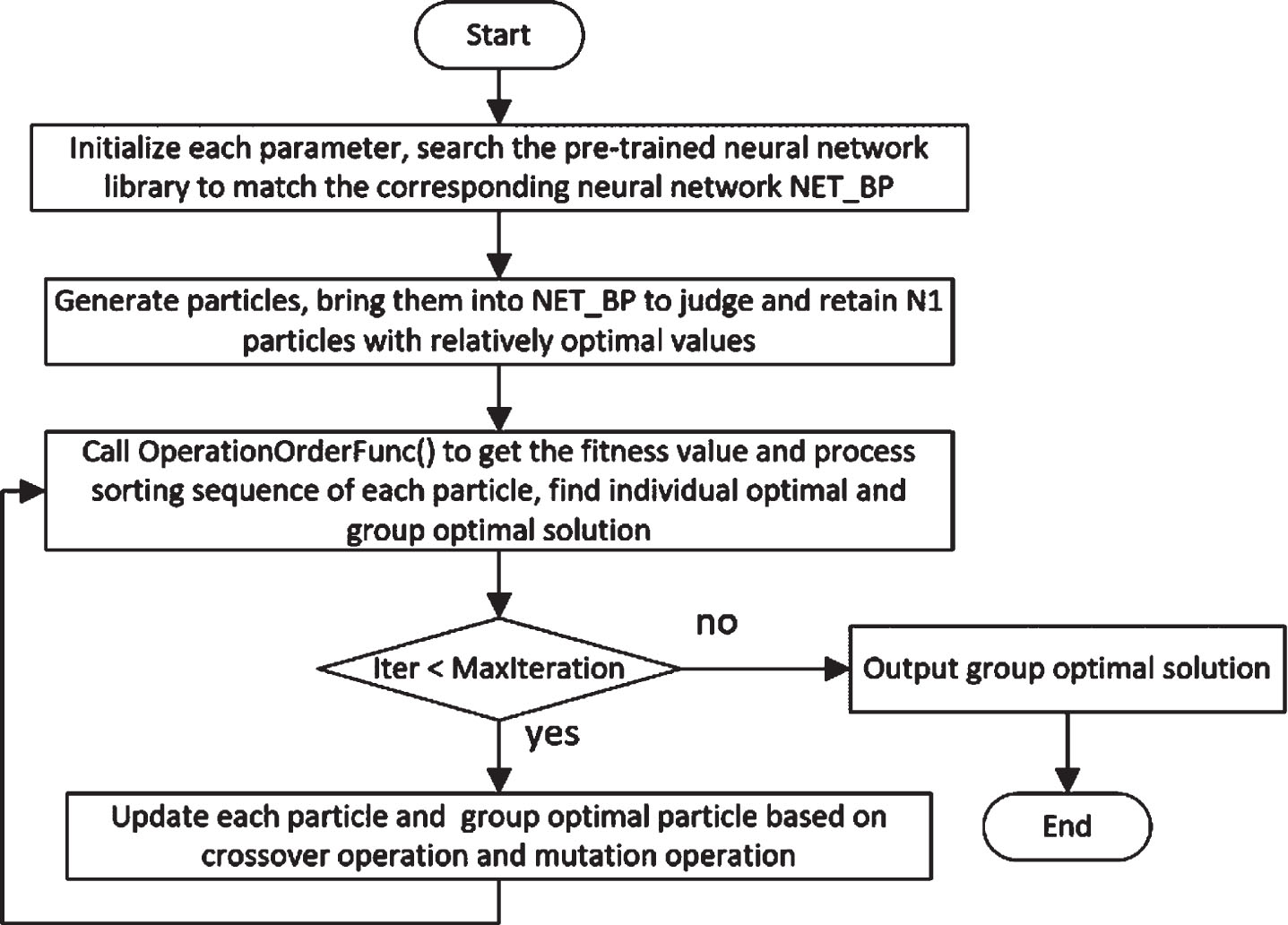
Flow chart of the BP-GA-PSO algorithm for the FJSP.

Fig. 2

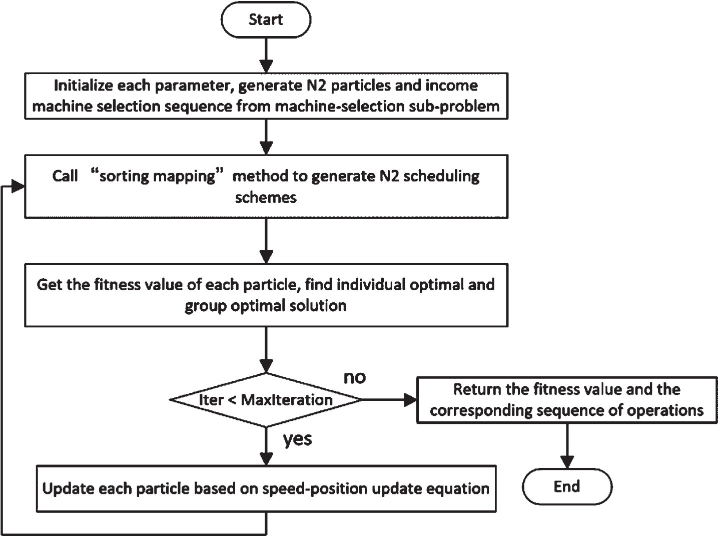
Flow chart of the operation-order sub-problem (OperationOrderFunc).

5 The BP-GA-PSO algorithm for the FJSP

5.1 GA for machine-selection sub-problem

5.1.1 Coding design

To apply a GA successfully to solve the FJSP, an appropriate representation of the particles is essential. For the machine-selection sub-problem in this study, a particle was represented by a chromosome (gene sequence) consisting of a machine-selection sequence. For the problem in Table 1, a gene sequence for machine selection can be expressed as [1 4 2 5 2 6 1 4 5 3 2 3], which means that operation O₁₁ of job J₁ selects machine m1 for processing, operation O₁₂ of J₁ selects machine m4 for processing, operation O₁₃ of J₁ selects machine m2 for processing, operation O₂₁ of J₂ selects machine m5 for processing, and the others have the same meaning.

Table 1
A FJSP (4×5 Kacem instance)

Job Operation Optional machine and processing time

M1 M2 M3 M4 M5

J₁ O₁₁ 2 5 4 1 2

O₁₂ 5 4 5 7 5

O₁₃ 4 5 5 4 5

J₂ O₂₁ 2 5 4 7 8

O₂₂ 5 6 9 8 5

O₂₃ 4 5 4 54 5

J₃ O₃₁ 9 8 6 7 9

. O₃₂ 6 1 2 5 4

O₃₃ 2 5 4 2 4

O₃₄ 4 5 2 1 5

J₄ O₄₁ 1 5 2 4 12

O₄₂ 5 1 2 1 2

Job	Operation	Optional machine and processing time
J₁	O₁₁	2	5	4	1	2
	O₁₂	5	4	5	7	5
	O₁₃	4	5	5	4	5
J₂	O₂₁	2	5	4	7	8
	O₂₂	5	6	9	8	5
	O₂₃	4	5	4	54	5
J₃	O₃₁	9	8	6	7	9
.	O₃₂	6	1	2	5	4
	O₃₃	2	5	4	2	4
	O₃₄	4	5	2	1	5
J₄	O₄₁	1	5	2	4	12
	O₄₂	5	1	2	1	2

5.1.2 Crossover operation

Crossover operation is one effective method of particle updating. Specifically, the particles are updated by exchanging fragments with the group-optimal particles. Two positions are randomly selected on the individual chromosome as marked points, and then the fragments between the marked points are exchanged with the group-optimal chromosomes at the same position. This method ensures that the descendants have legal sequences. Assume that the marked points are 5 and 10, respectively. The crossover operation is illustrated in Fig. 3.

Fig. 3

Crossover operation.

5.1.3 Mutation operation

For the machine-selection sub-problem, because each operation can be performed by more than one machine, n operations are randomly chosen, and each of the n operations reselects the machine number. The reselected machine number is placed in the corresponding machine-based sequence. To ensure the global nature of the mutation, each reselected machine number for each gene can still be the previous number after the mutation. The gene sequences obtained using this method ensure a legal solution. For example, if n = 2 and the randomly selected operations corresponding to the gene sequence number are two and five, the method is as shown in Fig. 4.

Fig. 4

Mutation operation.

5.2 PSO for operation-order sub-problem

5.2.1 Coding design

The operation-based coding method is generally adopted to ensure that the algorithm can obtain globally optimal solutions of the job-shop scheduling problem and has better performance [42].

Operation-based coding represents each operation sequence, and each gene sequence (chromosome) represents a scheduling scheme. All steps of the same job are represented by the same serial number, which is an integer from 1 to n that appears in the gene sequence.

The number of genes encoding this part of the chromosome is equal to the total number of operations, and the operation of each job is represented by the corresponding job number. The number of times the job number appears is equal to the number of job operations. Compiling is performed according to the order in which job numbers appear on the chromosome. Scanning the chromosome from left to right, the kth occurrence of the job number indicates the kth job operation. For the flexible job-shop scheduling problem presented in Table 1, a gene sequence based on the operation code can be expressed as [3 3 4 1 2 3 2 2 4 4 1 1], where 1 indicates an operation of job J₁ and 2, 3, and 4 have the same meaning. The three 1 s in the gene sequence represent the three operations of job J₁: operations 1, 2, and 3, respectively.

5.2.2 Update strategy for position and velocity vectors

In the standard particle swarm algorithm, the particle position and velocity are updated according to Equations (8) and (9) [43], respectively:

$\begin{matrix} V_{i}^{k + 1} = {wV}_{i}^{k} + c_{1} rand () ({pB}_{i}^{k} - X_{i}^{k}) \\ + c_{2} rand () ({gB}_{i}^{k} - X_{i}^{k}) \end{matrix}$ (8) $X_{i}^{k + 1} = X_{i}^{k} + V_{i}^{k + 1}$ (9)

In the above formulas, rand() is a random number generator, a random number in the interval (0, 1) occurs, w is an inertia factor of the degree of influence of the current speed on the speed of the next moment, and c₁ and c₂ are acceleration constants.

The updating of the position and velocity in the standard PSO algorithm is the key to the algorithm, but it is designed for the optimization of problems in the continuous domain. It does not apply to the JSP, which is a discrete-domain problem. Therefore, many researchers have changed this step. The most widely used method is to treat a chromosome as a particle directly and then to introduce the steps of the GA to crossover, mutate, and select the chromosome to transform a continuous problem into a discrete problem. The entire process is too complicated and does not take full advantage of the PSO. This paper proposes a scheduling sequence generation method, called “sorting mapping,” while maintaining the accuracy of PSO. The particle updating process still uses Equations (8) and (9) and runs in a continuous space.

Taking the problem of three jobs with two operations for each job as an example, this work introduce the following method.

$\begin{matrix} V_{i}^{k + 1} = {wV}_{i}^{k} + c_{1} rand () ({pB}_{i}^{k} - X_{i}^{k}) \\ + c_{2} rand () ({gB}_{i}^{k} - X_{i}^{k}) \end{matrix}$ (10) $X_{i}^{k + 1} = X_{i}^{k} + V_{i}^{k + 1}$ (11) $[A_{i}^{k}, B_{i}^{k}] = sort (X_{i}^{k})$ (12) ${array}_{i}^{k} = ceil (B_{i}^{k} / M)$ (13)

Step 1: Randomly generate 3*2 unequal real numbers in the interval (0, 1), and suppose that one of the particles is $X_{i}^{k} = [x_i_k_1, x_i_k_2, x_i_k_3, x_i_k_4, x_i_k_5, x_i_k_6]$ . In numerical terms, $X_{i}^{k}$ =[0.8825, 0.4073, 0.8266, 0.6096, 0.8844, 0.4378].

Step 2: The sort() function in Equation (10) sorts the six real numbers in $X_{i}^{k}$ from small to large and obtains $A_{i}^{k}$ =[0.4073, 0.4378, 0.6096, 0.8266, 0.8825, 0.8844] and $B_{i}^{k}$ =[2, 6, 4, 3, 1, 5], which is the index value of $A_{i}^{k}$ corresponding to $X_{i}^{k}$ , the ceil() function in Equation (11) obtains the largest integer not less than the argument, M is the maximum number of operations for each job (for jobs that are not up to the maximum number of operations, a virtual operation, i.e., an operation with a processing time of zero can be introduced; owing to limited space, no more tautology is given here), and ${array}_{i}^{k}$ =[1 3 2 2 1 3], which is a scheduling scheme.

Step 3: According to the position and velocity updating formulas of the PSO (Equations (8) and (9)), $X_{i}^{k + 1} = [x_i_(k + 1)_{1}, x_i_(k + 1)_{2}, x_i_(k + 1)_{3}, x_i_(k + 1)_{4}, x_i_(k + 1)_{5}, x_i_(k + 1)_{6}]$ can be calculated; that is, $X_{i}^{k + 1} = [1.2334, 0.5423, 1.3455, 0.4256, 0.5679, 0.9373]$ . Similarly, sorting the six real numbers in $X_{i}^{k + 1}$ from small to large gives $A_{i}^{k + 1}$ =[0.4256, 0.5423, 0.5679, 0.9373, 1.2334, 1.3455], and the index value of $A_{i}^{k + 1}$ corresponding to $X_{i}^{k + 1}$ is $B_{i}^{k + 1}$ =[4 , 3]. Then $B_{i}^{k + 1} / M$ is calculated and the numbers are rounded up toward positive infinity to obtain a sequence array _ i^k+1 = [213312], which is an updated scheduling scheme.

5.3 Reconstruction of the FJSP model based on JSON objection representation

For the machine-selection sub-problem, most of the running time of the algorithm is spent here because its iterative evolution is implemented by the value returned by the operation-order sub-problem. The initial population of the GA applied to the FJSP is randomly selected, which causes the algorithm to iterate many times to obtain optimal solutions. The method proposed in this study can obtain a better initial population, reducing the number of iterations to the optimal solutions. To determine the commonality between the optimal solutions of such FJSPs, this work introduce one of the most widely used machine learning methods, the BP neural network. Accordingly, it is necessary to generate samples, extract features, and train the BP neural network to make effective use of the generated BP neural network to predict optimal solutions. Most importantly, a method of clustering and reconstructing the FJSPs is necessary. Considering that JSON can conveniently and intuitively describe a class of problems and has the advantage of wide use in industrial scenarios, this work introduced JSON into this method. This study performed model reconstruction for the FJSP, called the JSON-FJSP.

The following is a JSON-FJSP:

{

“jobNumber”: IJobNum,

“machineNumber”: IMachineNum,

“validatedMaxProcessingTime”:

IMaxProcessingTime,

“operationList”: [

IJ₁,

IJ₂,

. . .

IJ_IJobNum

]

}

The corresponding descriptions of each field of the JSON-FJSP are shown in Table 2.

Table 2
Description of each field of a JSON-FJSP

Field of a JSON-FJSP Description

jobNumber job number

machineNumber machine number

validatedMaxProcessingTime max processing time of all operations

operationList the collection of the number of operations for each job

Field of a JSON-FJSP	Description
jobNumber	job number
machineNumber	machine number
validatedMaxProcessingTime	max processing time of all operations
operationList	the collection of the number of operations for each job

For the “operationList” field, the following conditions need to be met: $I J_{n} \leq I J_{n + 1} (0 < n \leq IJobNum)$

A JSON-FJSP is a series of FJSPs in which individual FJSPs can be constructed. These individual FJSPs can be used as samples to train the neural network. Such a neural network can be applied to the optimization of the JSON-FJSP.

To introduce the methodology proposed in this paper conveniently, this work used the JSON-FJSP as the research object called JSON-FJSP_Sample1 temporarily. The 4×5 Kacem instance belongs to JSON-FJSP_Sample1.

{

“jobNumber”: 4,

“machineNumber”: 5,

“validatedmMaxProcessingTime”: 12,

“operationList”: [

]

}

5.4 Optimization principle of BP-GA-PSO algorithm

The following is a comparison of the initial solution generation process of the GA-PSO algorithm without BP neural network filtering with that of the GA-PSO algorithm after BP neural network filtering. Taking a one-dimensional particle as an example, this work generated six one-dimensional particles. As can be seen from Fig. 5, because the unfiltered initial solution is randomly generated, the positions of these six particles are randomly distributed, and the positions corresponding to their fitness values are far from the optimal position, which means that more iterations are required to reach the optimal position in the later evolution process.

Fig. 5

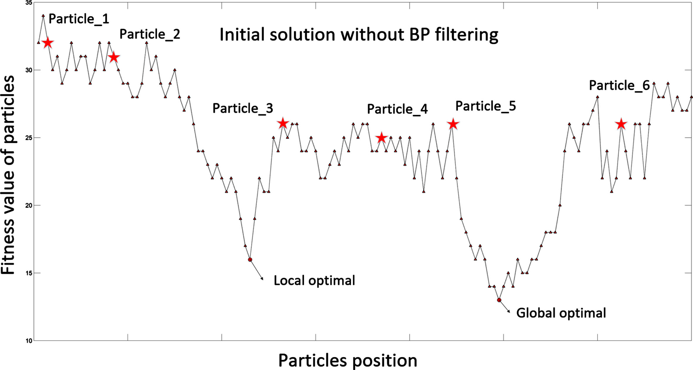
Initial solution generation process of the PSO algorithm without BP neural network filtering.

As shown in Fig. 6, the filtered particles are distributed in better positions, that is, the positions of the sub-optimal solution mentioned in the paper. They only require a few iterations, that is, short moving distances, to reach the optimal position.

Fig. 6

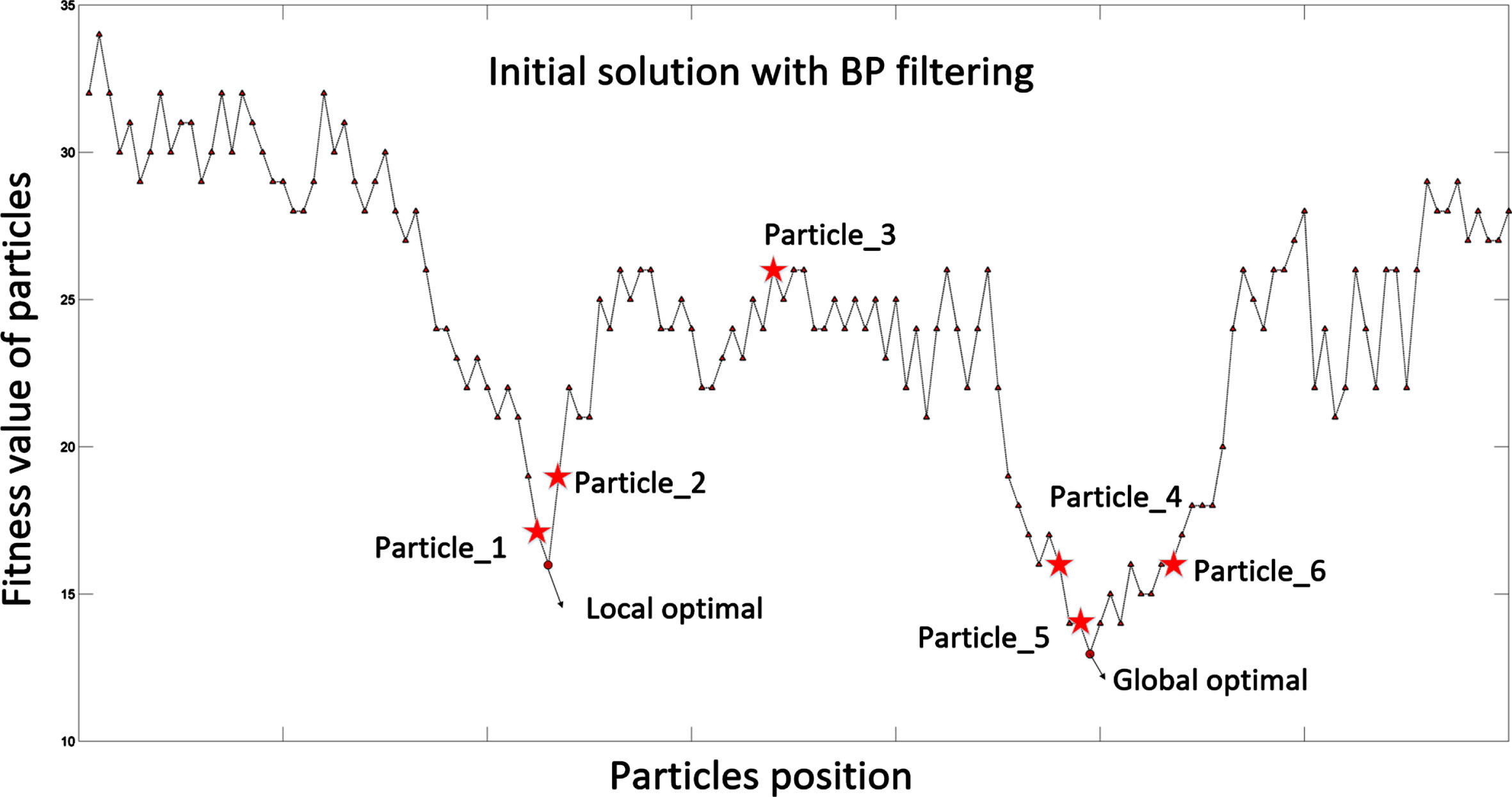
Initial solution generation process of the PSO algorithm after BP neural network filtering.

The proposed algorithm can also ensure the globality of the results and avoid falling into local optimal solutions through partial filtering. For example, as shown in Fig. 6, this work only filter out five of these six particles to make them suboptimal solutions; particle 3 is randomly generated, and the generation of particle 3 guarantees globality. In fact, it is not necessary to filter out many suboptimal solutions because a few suboptimal solutions can cause the particle swarm to move to the optimal solution position faster. Simultaneously, the filtration cost can be reduced.

The particles for solving the FJSP in this study are multi-dimensional, but the principle is the same as that described above.

5.5 BP neural network training

5.5.1 Feature extraction

This section discusses the identification of features that determine whether a solution is relatively optimal, considering the generation of random scheduling problems for JSON-FJSP_Sample1.

For JSON-FJSP_Sample1, this work constructed 10 FJSPs, of which 6 FJSPs were used as training sets, and 4 FJSPs were used as test sets. For each FJSP, a processing time t_i,j (1 ≤ t_i,j ≤ 12) was randomly generated on each machine for each operation. The solutions obtained by the six scheduling problems were different; therefore, the concept of the “relatively optimal-solution interval” was introduced. For a certain scheduling problem P(i), the completion time of its corresponding optimal solution is Tbest(i), and the completion time of a suboptimal solution is Tsub(i); then, the “relatively optimal-solution coefficient” is U = Tsub(i)/Tbest(i) and the relatively optimal-solution interval is [1, U].

The solution in the relatively optimal-solution interval is regarded as a good solution and marked as 1, and a solution that is not in the relatively optimal-solution interval is regarded as a bad solution and marked as 0. This process constructs a model that applies neural networks to solve classification problems, and the relatively optimal-solution interval is applicable to any scheduling problem in the JSON-FJSP. In this study, through multiple data attempts and verifications, 1.4 was chosen as the relatively optimal-solution coefficient for JSON-FJSP_Sample1, and the experimental verification process will be given later.

Six hundred machine-selection sequences were generated for each FJSP. Some were in the relatively optimal-solution interval, and the others were not. The 600 machine-selection sequences were converted into 600 training samples under the corresponding features of each scheduling problem, for a total of 3600 training samples.

Because this work regarded minimizing the completion time as the scheduling target, the feature selection was directly or indirectly related to time. Because which features were useful were not known at the beginning, this work listed as many features as possible. Next, this work extracted features that were useful for solving the problem.

The feature selection path map (FSP) and sparse-error contrast curve (SET) are two useful visual tools proposed by Benoít et al. [44] to assist feature extraction effectively. As shown in the left part of Fig. 7, the FSP displays the best feature subset for each subset size, with each column corresponding to a subset size and blue cells corresponding to the selected features. The SET on the right side of Fig. 7 shows the error for the corresponding feature subset. From these images, a suitable subset of the features can be selected. These diagrams indicate which features are useful for obtaining the correct results and which features are not worth extracting. The features obtained in this study are listed in Table 3, and the corresponding descriptions are as follows:

Fig. 7

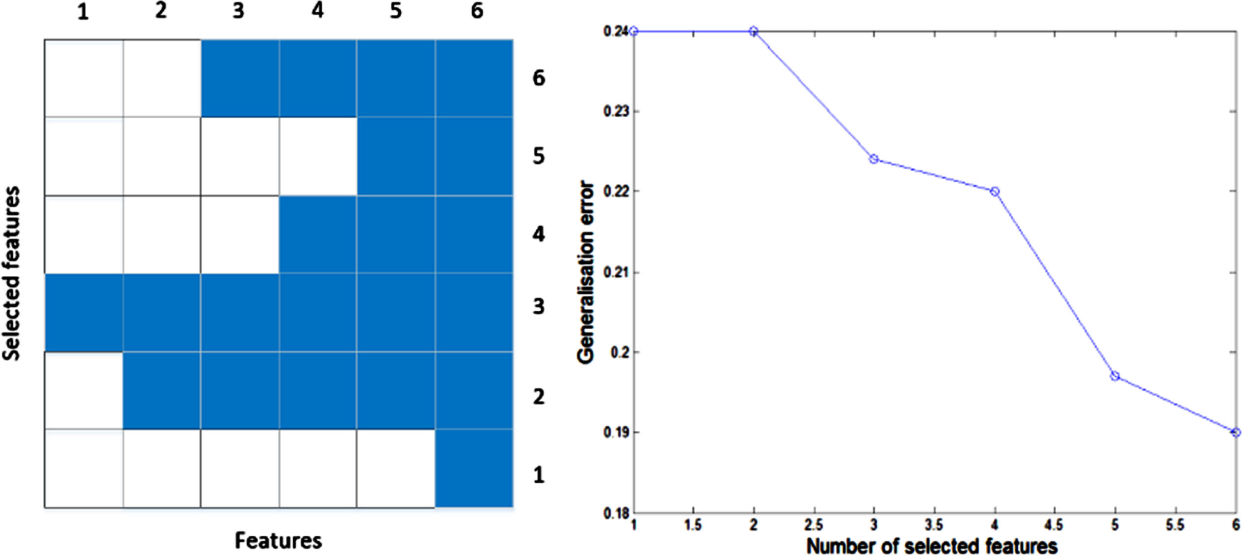
Feature Selection Path Map (FSP) and Sparse-Error Contrast Curve (SET) for feature extraction.

Table 3

Features that have been obtained in this paper

Feature	Formula description
Feature 1	D(count(i)/(2^{count _ min(i)}))
Feature 2	T_{sum _ chose}/T_sum
Feature 3	count_{min _ machine _ times}/count_times
Feature 4	T_{max _ chose}/T_{min _ chose}
Feature 5	T_{max _ chose}/T_{second _ max _ chose}
Feature 6	count_{samejob _ samemachine}/count_{sum _ operations}

Feature 1: For a certain machine-selection sequence and its corresponding scheduling problem matrix T, count(i) is the number of times i appears in the sequence, count_min(i) is the number of times i corresponds to the shortest time in T, and Feature 1 is D(count(i)/(2^{count _ min(i)})), where the function D() represents the variance.

Feature 2: T_{sum _ chose} is the total processing time of selected machines, T_sum is the total time of T, and Feature 2 is T_{sum _ chose}/T_sum;

Feature 3: count_{min _ machine _ times} is the number of times each operation of selecting the machines with the shortest processing time is performed, count_times is the number of all operations, and Feature 3 is count_{min _ machine _ times}/count_times.

Feature 4: the maximum processing time of the selected machines divided by the minimum processing time of the selected machines.

Feature 5: the maximum processing time of the selected machines divided by the second maximum processing time of the selected machines.

Feature 6: the number of times the same job selects the same machine, divided by the total number of operations.

This work randomly generated 3600 samples of six problems for neural network training and then randomly generated the seventh problem for prediction. The FSP and SET were drawn by implementing the prediction process for the seventh problem, as shown in Fig. 7. The detailed training and prediction processes are presented in the Subsection 5.2.2.

As can be seen from Fig. 7, as the number of features increases, the prediction error decreases; thus, all features obtained previously should be retained.

5.5.2 Training strategy for BP neural network

The model used in this study was a three-layer BP neural network. The error BP algorithm was used to learn the neural network model. The BP neural network structure is shown in Fig. 8 [45]. In the figure, the input layer contains m neurons corresponding to X={x₁, x₂,..., x_m}, the number of neurons in the hidden layer is n, and the output layer is a single neuron (whether it is a relatively optimal solution). The values of m and n are assigned later.

Fig. 8

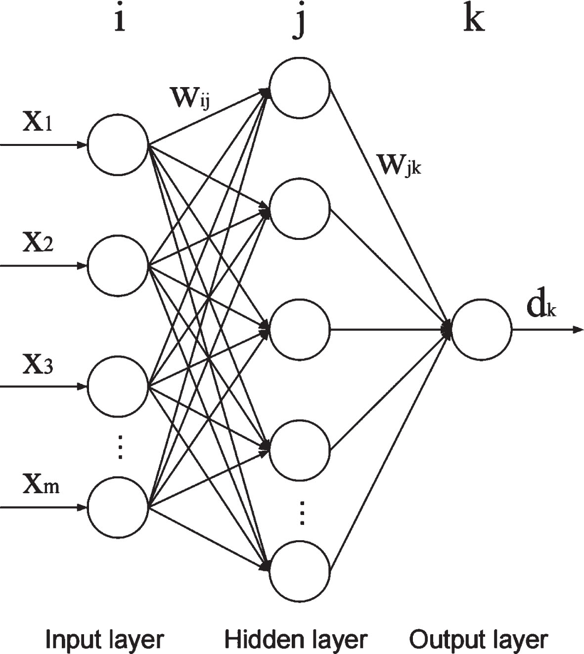
Three-layer BP neural network structure.

The input parameter set for the model was obtained by converting the machine-selection sequences into training samples under the corresponding features. However, because different feature parameters have different units and orders of magnitude, in order to eliminate the influence of different units and data magnitudes on the model prediction results, data normalization was performed before the parameters are input into the network model to ensure that the parameters were of the same order of magnitude [46]. Normalization was implemented using the calculation method shown in Equation (12), where X represents the current value; X_min and X_max represent the minimum and maximum values, respectively; and Y is the normalized value. The normalized data range is [0, 1]. $Y = \frac{X - X_{\min}}{X_{\max} - X_{\min}}$ (14)

The training and test sets were carefully designed. Neural network training was performed using 3600 samples generated by six problems, and Test 1, Test 2, and Test 3 were randomly generated; Test 4 was the 4×5 Kacem instance. Each problem yielded 600 solutions. These problems were divided into four groups for the prediction.

These problems are presented in Table 4. The prediction results and related experimental data are as follows.

Table 4

Tale 4 Training sets and test sets of JSON-FJSP_Sample1

		Mathematical model represented by a matrix model
Train sets	Train1	[2,3,2,5,4; 9,6,6,11,5; 3,8,4,5,2; 4,6,11,10,8; 5,10,8,1,5; 12,5,10,1,3; 3,4,9,8,6; 4,7,3,6,5; 6,8,3,11,7; 7,3,2,7,6; 8,12,9,4,5; 5,8,10,6,1]
	Train2	[11,8,6,7,8; 12,3,6,11,1; 10,7,1,1,2; 6,6,12,10,8; 7,10,10,1,5; 12,5,2,1,3; 1,4,9,7,6; 8,7,3,8,9; 9,6,3,11,5; 8,3,2,6,6; 8,12,9,4,10; 4,8,10,6,1]
	Train3	[5,3,6,2,8; 12,3,6,9,1; 10,7,10,1,2; 6,6,12,10,8; 6,5,5,9,5; 8,6,4,2,3; 1,4,9,7,6; 4,7,3,8,9; 9,6,3,11,5; 5,3,2,6,6; 7,12,9,4,10; 3,7,9,7,2]
	Train4	[8,3,5,6,7; 2,2,7,2,5; 8,9,6,2,10; 9,10,5,1,4; 2,2,2,10,9; 2,8,2,2,2; 3,4,11,7,9; 4,2,7,12,8; 12,5,8,5,2; 7,9,10,8,4; 9,7,2,6,6; 12,6,3,10,10]
	Train5	[1,9,10,9,4; 4,9,3,9,9; 2,3,12,10,2; 3,4,5,10,7; 1,7,12,6,5; 8,9,5,12,12; 7,5,11,9,4; 12,6,10,9,5; 8,3,4,9,5; 11,9,4,6,3; 6,5,11,10,7; 9,8,9,3,5]
	Train6	[8,11,7,2,9; 7,11,8,1,8; 1,12,2,9,6; 12,3,1,7,10; 10,3,4,10,4; 4,6,6,10,6; 2,3,2,2,9; 8,6,7,11,4; 4,4,2,2,11; 5,1,1,7,10; 8,1,9,2,1; 2,3,2,10,3]
Test sets	Test1	[4,8,10,4,6; 5,3,8,11,1; 12,7,10,11,9; 7,6,12,10,8; 7,3,4,1,5; 6,4,2,1,2; 2,4,7,7,6; 5,7,3,5,9; 8,6,3,6,5; 1,3,2,3,4; 7,12,9,4,10; 4,8,7,6,3]
	Test2	[2,1,4,4,7; 12,7,4,6,7; 10,5,11,10,8; 3,7,8,7,10; 5,9,2,7,7; 6,5,5,9,10; 2,5,1,6,8; 3,7,9,2,7; 7,8,1,6,10; 10,2,11,7,1; 1,8,10,8,7; 6,12,7,11,8]
	Test3	[3,9,2,5,6; 9,1,9,6,11; 2,6,1,10,10; 4,3,12,1,10; 6,9,11,7,8; 11,10,8,12,1; 5,12,4,7,5; 6,9,5,8,6; 6,11,6,6,9; 5,1,3,11,2; 3,6,1,12,8; 6,8,6,1,3]
	Test4	[2,5,4,1,2; 5,4,5,7,5; 4,5,5,4,5; 2,5,4,7,8; 5,6,9,8,5; 4,5,4,54,5; 9,8,6,7,9; 6,1,2,5,4; 2,5,4,2,4; 4,5,2,1,5; 1,5,2,4,12; 5,1,2,1,2]

Each problem in the training sets (Train 1–6) had 600 samples, of which 470 were used to train neural networks (70% of 470 samples were training sets, 15% were test sets, 15% were validation sets), and 130 were used for prediction. The three randomly generated problems (Test 1–3) and the problem of the 4×5 Kacem instance (Test 4) were used as prediction sets. Table 5 shows that the trained BP neural network has an extremely high predictive accuracy of approximately 91%. That is, with this trained BP neural network, one can determine in advance whether a solution is good or bad with approximately 91% accuracy.

Table 5

Prediction results

	Training sets						Test sets
	Train1	Train2	Train3	Train4	Train5	Train6	Test1	Test2	Test3	Test4
Optimal solution	12	16	13	11	15	9	14	13	16	11
Number of relatively optimal
solutions/relatively bad solutions	199/401	211/389	274/256	267/333	242/358	144/456	289/311	235/365	310/290	275/325
Accuracy of relatively optimal solution (%)							89.73	93.22	89.75	90.00
Accuracy of relatively bad solution (%)							86.67	92.37	93.72	93.75

5.6 Influence of relatively optimal-solution coefficient on predictive accuracy

The relatively optimal-solution coefficient is used for solution classification, which directly affects the predictive accuracy. If the relatively optimal-solution coefficient is too small to be close to 1, all the relatively optimal solutions will be optimal solutions. Because the number of optimal solutions in the sample is not large, the features of the optimal solutions cannot be learned sufficiently. If the relatively optimal-solution coefficient is too large, then the features of the relatively optimal solutions will be overwhelmed, and the relatively optimal solutions will not be distinguished well. Therefore, the optimal solution coefficient should be chosen appropriately. The following describes the relationship between the relatively optimal-solution coefficient and predictive accuracy.

Figure 9 shows that when the relatively optimal-solution coefficient is 1.4, the predictive accuracy of the relatively optimal solutions, predictive accuracy of the relatively bad solutions, and overall predictive accuracy are all relatively high, so this value is the best in all respects. Therefore, the relatively optimal-solution coefficients of all experimental data in this study were set to 1.4.

Fig. 9

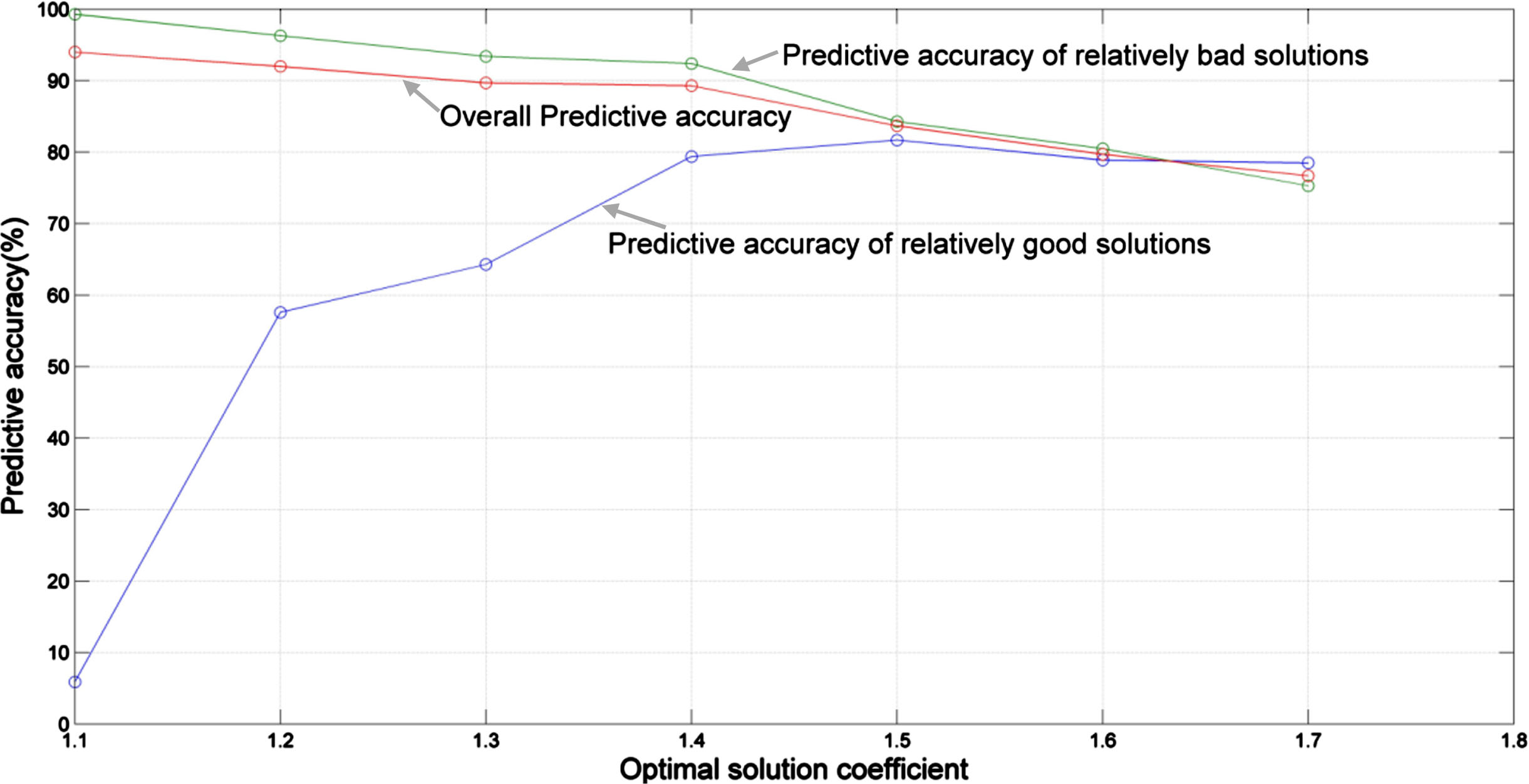
Relationship between the relatively optimal-solution coefficient and predictive accuracy.

6 Computation results

6.1 BP neural network performance test

To test the performance of the BP neural network obtained previously, this work compared BP-GA-PSO and GA-PSO on the 4×5 Kacem instance (Test 4), as shown in Table 6. Furthermore, this work performed the comparison between BP-GA-PSO and MOGA on the the 4×5 Kacem instance (Test 1), as shown in Table 7. BP neural network is the machine learning method introduced in this study. This work verified the effectiveness of the machine learning method by comparing the performance of the algorithm with and without a BP neural network. The former is BP-GA-PSO, and the latter is GA-PSO. The parameter values were as follows: the initial population number was 100, the number of iterations was 200, and the neural network was the single hidden layer neural network described in the previous section. The number of input layer neurons m was six, the number of hidden layer neurons n was 25, and the relatively optimal-solution coefficient U was 1.4.

Table 6
Initial solutions and results comparison of Test4

GA-PSO BP-GA-PSO

Relatively-optimal-solution coefficient N/A 1.4

C_max 11 11

Fitness values of initial population (top 20 out of 100) [29,65,23,22,22, 21,25,24,23,21, 70,70,27,20,28, 20,19,29,21,66] [15,16,15,15,13, 14,15,14,14,16, 28,14,14,14,16,23, 25,22,13,14]

Number of relatively optimal solutions 0 16

Wilcoxon W 251

Asymp. Sig. (2-tailed) <0.001

	GA-PSO	BP-GA-PSO
Relatively-optimal-solution coefficient	N/A	1.4
C_max	11	11
Fitness values of initial population (top 20 out of 100)	[29,65,23,22,22, 21,25,24,23,21, 70,70,27,20,28, 20,19,29,21,66]	[15,16,15,15,13, 14,15,14,14,16, 28,14,14,14,16,23, 25,22,13,14]
Number of relatively optimal solutions	0	16
Wilcoxon W	251
Asymp. Sig. (2-tailed)	<0.001

Table 7

Initial solutions and results comparison of Test1

	MOGA	BP-GA-PSO
Relatively-optimal-solution coefficient	N/A	1.4
C_max	14	14
Fitness values of initial population (top 20 out of 100)	[28,35,32,24,38,25, 24,27,23,28,28,30,42, 41,38,32,39,39,26,27]	[15,16,15,20,18,18, 19,22,17,19,19,22,18, 17,17,23,19,17,17,20]
Number of relatively optimal solutions	0	17
Wilcoxon W	210.5
Asymp. Sig. (2-tailed)	<0.001

For the 4×5 Kacem instance (Test 4), C_max is 11, and the corresponding fitness value of the relatively optimal-solution is ceil (11*1.4) (the ceil() function obtains the largest integer not less than the argument), yielding 16 as the fitness value of the relatively optimal-solution. This work used GA-PSO and BP-GA-PSO to generate 100 initial solutions, and the fitness values of the first 20 initial solutions are listed Table 6. Sixteen of the initial solutions obtained by BP-GA-PSO are relatively optimal, whereas the number of relatively optimal solutions among the initial solutions obtained by GA-PSO is 0. In other words, the initial population of BP-GA-PSO is much better than that of GA-PSO because the BP neural network has judged the initial solutions in advance and maintains the relatively optimal solutions. In addition, the BP-GA-PSO results are statistically investigated with the Wilcoxon rank-sum test, the Wilcoxon W is 251 and the asymptotic significance is less than 0.001 which means the data obtained by BP-GA-PSO differs significantly from the one by GA-PSO.

For the 4×5 Kacem instance (Test 1), C_max is 14, and the corresponding fitness value of the relatively optimal-solution is ceil (14*1.4) (the ceil() function obtains the largest integer not less than the argument), yielding 20 as the fitness value of the relatively optimal-solution. This comparison used BP-GA-PSO and GA-PSO to generate 100 initial solutions, and the fitness values of the first 20 initial solutions are listed Table 7. Seventeen of the initial solutions obtained by BP-GA-PSO are relatively optimal, whereas the number of relatively optimal solutions among the initial solutions obtained by MOGA is 0. In other words, the initial population of BP-GA-PSO is much better than that of MOGA because the BP neural network has judged the initial solutions in advance and maintains the relatively optimal solutions. Furthermore, the BP-GA-PSO results are statistically investigated with the Wilcoxon rank-sum test, the Wilcoxon W is 210.5 and the asymptotic significance is less than 0.001 which means the data obtained by BP-GA-PSO differs significantly from the one by MOGA.

6.2 Comparison of BP-GA-PSO success rates

To test the performance of BP-GA-PSO further, this work compared its results with those of other well-known algorithms using two sets of benchmark studies: ten BRdata instances [4] and five Kacem instances.

For the first set of data, the BRdata instances, this work repeatedly ran BP-GA-PSO 10 times and listed the best results. Table 8 compares the makespans of the optimal solutions of BP-GA-PSO and those in the literature (TS [4], PVNS [47], MOGA [48], PSO+TS [30], and P-EDA [49]). For the ten instances of BRdata, the best results obtained by BP-GA-PSO are equal to or less than those obtained by other algorithms. For the MK01 instance, BP-GA-PSO outperforms TS and is on par with the other four algorithms. For instance, in MK02, the BP-GA-PSO outperformed TS, PSO+TS, and MATSLO. For instance, in MK03, BP-GA-PSO outperformed TS and MATSLO. For the MK04 instance, the makespan 60 obtained by the BP-GA-PSO dominates the other four algorithms, as the PVNS does. For MK05 and MK06, the BP-GA-PSO outperforms the others. For M07, the BP-GA-PSO gets the makespan 139 which equals the one by MOGA and is better than the other four algorithms. For MK08, our algorithm and the others get the same result. For M09, the BP-GA-PSO gets the makespan 307 which equals the one by PVNS and is better than the other four algorithms. For MK10, our algorithm is a little worse than PVNS, but is better than the other four algorithms.

Table 8
Comparison of results on Bandimarte instances

TS PVNS MOGA PSO+TS MATSLO BP-GA-PSO

MK01 42 40 40 40 40 40

MK02 32 26 26 27 32 26

MK03 211 204 204 204 207 204

MK04 81 60 62 63 67 60

MK05 186 173 173 173 188 172

MK06 86 60 62 65 85 58

Mk07 157 141 139 145 154 139

MK08 523 523 523 523 523 523

MK09 369 307 310 331 437 307

MK10 296 208 214 223 380 212

	TS	PVNS	MOGA	PSO+TS	MATSLO	BP-GA-PSO
MK01	42	40	40	40	40	40
MK02	32	26	26	27	32	26
MK03	211	204	204	204	207	204
MK04	81	60	62	63	67	60
MK05	186	173	173	173	188	172
MK06	86	60	62	65	85	58
Mk07	157	141	139	145	154	139
MK08	523	523	523	523	523	523
MK09	369	307	310	331	437	307
MK10	296	208	214	223	380	212

For the second set of data, the Kacem instances, this work repeatedly ran BP-GA-PSO 10 times and listed the best results.

Table 9 compares the best and average values between BP-GA-PSO and those in the literature (AL+CGA [50], BBO [51], BEDA [52], KBACO [53], ABC [54], HDE-N2 [55] and SEA [56]). In Table 9, the following notations are used:

Table 9

Comparison result for the Kacem instances

Instance	Job×Machine	C ^*	AL+CGA		BBO		BEDA		KBACO
			C_max	AVG	C_max	AVG	C_max	AVG	C_max	AVG
Kacem 1	4×5	11	16	N/A	11	11	11	11	11	11
Kacem 2	8×8	14	15	N/A	14	14.75	14	14	14	14.3
Kacem 3	10×7	11	15	N/A	N/A	N/A	11	11	11	11
Kacem 4	10×10	7	7	N/A	7	7.75	7	7	7	7.4
Kacem 5	15×10	11	23	N/A	13	13	11	11	11	11.3
Instance	Job×Machine	ABC		HDE-N2		SEA		BP-GA-PSO
			C_max	AVG	C_max	AVG	C_max	AVG	C_max	AVG
Kacem 1	4×5	11	11	11	11	11	11	11	11
Kacem 2	8×8	14	14	14	14	14	14	14	14
Kacem 3	10×7	11	11	11	11	11	11	11	11
Kacem 4	10×10	7	7	7	7	7	7	7	7
Kacem 5	15×10	11	11	11	11	11	11	11	11

BBO: on a 2.4 GHz CPU and 4GB RAM. BEDA: on a 3.2 GHz CPU. KBACO: on a 2.4 GHz CPU and 1 GB RAM. TSPCB: on a 1.6 GHz CPU and 512 MB RAM. ABC: on a 2.83 GHz CPU and 3.21 GB RAM. BP-GA-PSO: on a 2.6 GHz CPU and 8.0 GB RAM. HDE-N2: on a 2.83 GHz CPU and 15.9 GB RAM.

C ^*	best known solution for makespan
C_max	best solution for makespan
AVG	average of the solution for makespan

From Table 9, it can be concluded that BP-GA-PSO is not worse than the other algorithms and is even better than several improved algorithms. Further, BP-GA-PSO can obtain an optimal solution with a 100% success rate.

Figure 10 compares BP-GA-PSO and several effective algorithms, including BBO [51] and MOGA [48], for a 10×7 Kacem instance. BP-GA-PSO can quickly obtain the best makespan with very few iterations.

Fig. 10

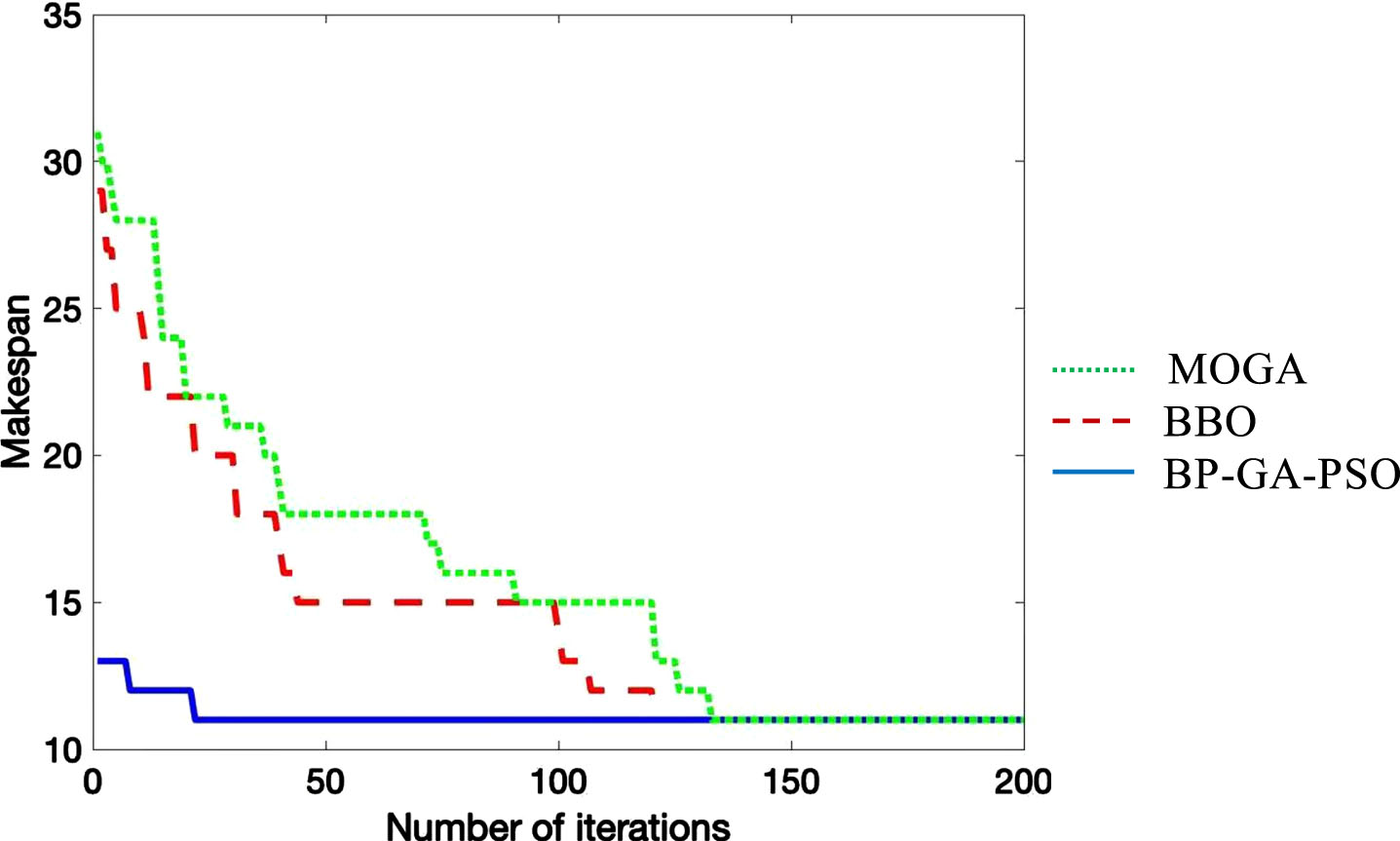
The comparison of convergence between MOGA, BBO and BP-GA-PSO on 10×7 Kacem instance.

Figures 11 and 12 show the Gantt charts of the optimal solutions obtained by BP-GA-PSO when solving the 4×5 and 10×10 instances, respectively. This work obtain 11, which is the makespan of the best-known solution for the 4×5 instance, and 7, which is the makespan of the best-known solution, for the 10×10 instance.

Fig. 11

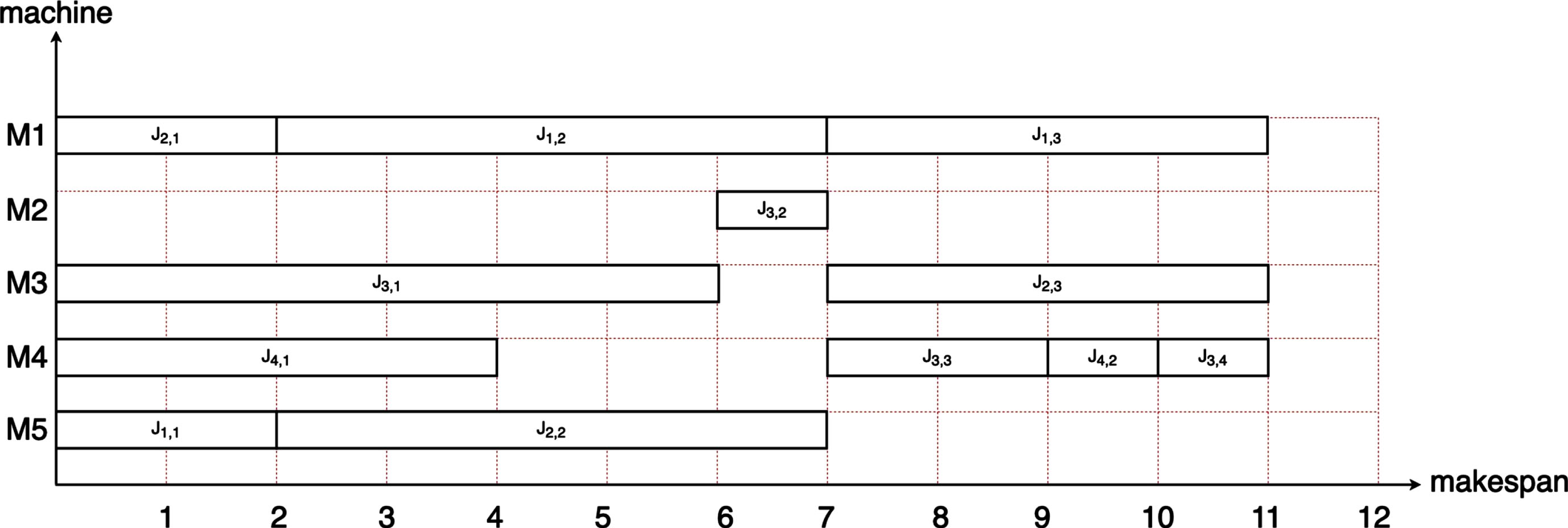
The Gantt chart of instance 1 (4×5).

Fig. 12

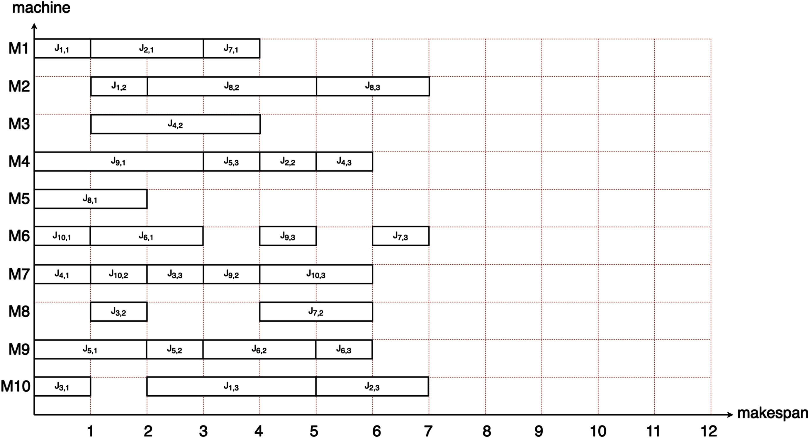
The Gantt chart of instance 4 (10×10).

7 Conclusion

This study addressed one of the most challenging combinatorial problems: the FJSP. The JSON-FJSP is proposed and a machine learning method to optimize the solutions is introduced. The FSP and SET were also introduced into the feature extraction process; thus, some valuable features were extracted. The pre-trained BP neural network was verified to optimize the initial population, accelerate the convergence of the algorithm, and improve the probability of convergence to the optimal solution.

The originality of this approach consists of reconstructing the mathematical model of the FJSP so that machine learning strategies can be introduced to optimize the algorithms for the FJSP. This reconstructed model (JSON-FJSP) seems to be a new direction for introducing more interesting methodologies to solve the FJSP. Thus far, many machine learning methods have provided scientific benefits, but these methods are rarely used to solve the FJSP. The BP-GA-PSO approach for the FJSP proposed in this study proved to be feasible and effective.

The approach proposed in this article can not only be applied to the FJSP with the goal of “shortest processing time”, but also to the FJSP with other goals, bringing a new optimization concept to the solution of these problems.

The disadvantage of this approach proposed in this paper is that a large number of sample training is required to obtain the corresponding BP neural networks before the algorithm is implemented. However, these trainings are done offline in advance, the efficiency of the algorithm is not affected.

References

Chaudhry

I.A.

and Khan

A.A.

, A research survey: review of flexiblejob shop scheduling techniques, International Transactions inOperational Research 23(3) (2015), 551–591.

Alburaikan

, Garg

and Khalifa

H.A.E.W.

, A novel approach for minimizing processing times of three-stage flow shop scheduling problems under fuzziness, Symmetry 15(1) (2023), 130.

Gao

K.Z.

, Cao

Z.G.

and Zhang

, A review on swarm intelligence and evolutionary algorithms for solving flexible job shop scheduling problems, IEEE/CAA JOURNAL OF AUTOMATICA SINICA 6(4) (2019), 904–916.

Brandimarte

, Routing and scheduling in a flexible job shop by tabu search, Annals of Operations Research 41(3) (1993), 157–183.

Zakarian

and Kusiak

, Process analysis and reengineering, Computers & Industrial Engineering 41(2) (2001), 135–150.

and Wu

, An elitist quantum-inspired evolutionary algorithm for the flexible job-shop scheduling problem, Journal of Intelligent Manufacturing 28(6) (2017), 1441–1457.

Kacem

, Genetic algorithm for the flexible job-shop scheduling problem. SMC’03 Conference Proceedings. IEEE International Conference on Systems, Man and Cybernetics. Conference Theme-System Security and Assurance (Cat. No. 03CH37483) 4(4) (2003), 3464–3469.

Chen

J.C.

, Wu

C.C.

, Chen

C.W.

and Chen

K.H.

, Flexible job shop scheduling with parallel machines using genetic algorithm and grouping genetic algorithm, Expert Systems with Applications 9(11) (2012), 10016–10021.

Zhan

Z.H.

, Shi

, Tan

K.C.

and Zhang

, A survey on evolutionary computation for complex continuous optimization, Artificial Intelligence Review 55(1) (2022), 59–110.

10.

Luo

G.F.

, Song

J.J.

, Zhang

Z.F.

and Li

J.C.

, Solving flexible job shop scheduling problem based on improved genetic algorithm, IOP Conference Series Materials Science and Engineering 394(3) (2018).

11.

Wang

Y.H.

, Fu

L.Q.

, Su

Y.Q.

, Yang

and Wu

L.F.

, Genetic algorithm in flexible workshop scheduling based on multi-objective optimization, Journal of Interdisciplinary Mathematics 21(5) (2018), 1249–1254.

12.

, Chen

, Gao

, Li

, Zhang

Multiobjective flexible job-shop rescheduling with new job insertion and machine preventive maintenance, IEEE Transactions on Cybernetics (2022), 1–13.

13.

Liu

S.C.

, Chen

Z.G.

, Zhan

Z.H.

, Jeon

S.W.

, Kwong

, Zhang

Many-objective job-shop scheduling: a multiple populations for multiple objectives-based genetic algorithm approach, IEEE Transactions on Cybernetics (2022), 1–15.

14.

Gao

, Peng

C.Y.

, Zhou

, Li

P.G.

Solving flexible job shop scheduling problem using general particle swarm optimization, Proceedings of the 36th CIE Conference on Computers & Industrial Engineering (2006).

15.

Ding

and Gu

, Improved particle swarm optimization algorithmbased novel encoding and decoding schemes for flexible job shopscheduling problem, Computers & Operations Research 121(3) (2020), 104951.

16.

X.L.

, Huang

and Liang

, A discrete particle swarm optimization algorithm with adaptive inertia weight for solving multiobjective flexible job-shop scheduling problem, IEEE Access 1(1) (2020), 99–112.

17.

Zhan

Z.H.

, Matrix-based evolutionary computation, IEEE Transactions on Emerging Topics in Computational Intelligence 6(2) (2022), 315–328.

18.

Jian

J.R.

, Chen

Z.G.

, Zhan

Z.H.

and Zhang

, Region encoding helps evolutionary computation evolve faster: a new solution encoding scheme in particle swarm for large-scale optimization, IEEE Transactions on Evolutionary Computation 1(1) (2021), 99.

19.

J.Y.

, Zhan

Z.H.

, Liu

R.D.

, Wang

, Kwong

and Zhang

, Generation-level parallelism for evolutionary computation: a pipeline-based parallel particle swarm optimization, IEEE Transactions on Cybernetics 51(10) (2021), 4848–4859.

20.

Xia

, Triple archives particle swarm optimization, IEEE Transactions on Cybernetics 50(12) (2020), 4862–4875.

21.

Wang

Z.J.

et al. Dynamic group learning distributed particle swarm optimization for large-scale optimization and its application in cloud workflow scheduling, IEEE Transactions on Cybernetics 50(6) (2022), 2715–2729.

22.

Huang

R.H.

, Yang

C.L.

and Cheng

W.C.

, Flexible job shop scheduling with due window-a two-pheromone ant colony approach, International Journal of Production Economics 141(2) (2013), 685–697.

23.

Rossi

, Flexible job shop scheduling with sequence dependent setup and transportation times by ant colony with reinforced pheromone relationships, International Journal of Production Economics 153 (2014), 253–267.

24.

Gao

and Pan

Q.K.

, A shuffled multi-swarm micro-migrating birds optimizer for a multi-resource-constrained flexible job shop scheduling problem, Information Sciences 372 (2016), 655–676.

25.

Kavitha

, Venkumar

, Rajini

and Pitchipoo

, An efficient social spider optimization for flexible job shop scheduling problem, Journal of Advanced Manufacturing Systems 17(2) (2018), 181–196.

26.

Chiang

T.C.

and Lin

H.J.

, A simple and effective evolutionaryalgorithm for multi-objective flexible job shop scheduling, International Journal of Production Economics 141(1) (2013), 87–98.

27.

Gao

K.Z.

, Yang

F.J.

, Zhou

M.C.

, Pan

Q.K.

and Sugnathan

P.N.

, Flexible job shop rescheduling for new job insertion by using discrete Jaya algorithm, IEEE TRANSACTIONS ON CYBERNETICS 49(5) (2019), 1944–1955.

28.

Garg

A hybrid GSA-GA algorithm for constrained optimization problems, Information Sciences (2019), 478.

29.

Kundu

, Garg

LSMA-TLBO: A hybrid ITLHHO algorithm for numerical and engineering optimization problems, International Journal of Intelligent Systems (2021), 37.

30.

, Pan

, Xie

, Jia

and Wang

, A hybrid particle swarmoptimization and tabu search algorithm for flexible job-shopscheduling problem, International Journal of Computer Theoryand Engineering 2(2) (2010), 189.

31.

Tang

J.C.

, Zhang

G.J.

, Lin

B.B.

and Zhang

B.X.

, A hybrid algorithmfor flexible job-shop scheduling problem, ProcediaEngineering 15 (2011), 3678–3683.

32.

Tang

H.T.

, Chen

, Li

Y.B.

, Peng

, Guo

S.S.

and Du

Y.Z.

, Flexible job-shop scheduling with tolerated time interval and limited starting time interval based on hybrid discrete PSO-SA: An application from a casting workshop, Applied Soft Computing 78 (2019), 176–194.

33.

Wang

, Yang

L.I.

and Xinyu

L.I.

, Solving flexible job shop scheduling problem by a multi-swarm collaborative genetic algorithm, Journal of Systems Engineering and Electronics 32(2) (2021), 261–271.

34.

, Gao

, Duan

P.Y.

, Li

J.Q.

, Zhang

An improved artificial bee colony algorithm with Q-learning for solving permutation flow-shop scheduling problems, IEEE Transactions on Systems, Man, and Cybernetics: Systems, 2022.

35.

Alawad

N.A.

, Abed-alguni

B.H.

Discrete jaya with refraction learning and three mutation methods for the permutation flow shop scheduling problem, The Journal of Supercomputing, 2022.

36.

Abed-alguni

B.H.

, David Paul , Island-based Cuckoo Search with elite opposition-based learning and multiple mutation methods for solving optimization problems, Soft Computing 26 (2022), 1–20.

37.

Alkhateeb

, Abed-alguni

B.H.

and Al-rousan

M.H.

, Discrete hybrid cuckoo search and simulated annealing algorithm for solving the job shop scheduling problem, The Journal of Supercomputing 78(4) (2022), 4799–4826.

38.

Ming

and Zheng

, Application of improved genetic algorithm based on machine learning in job shop scheduling, Machinery 42(11) (2004), 47–48.

39.

Gong

and Xiong

G.L.

, Application of machine learning in intelligent job shop scheduling system, Control and Decision 3 (1997), 32–37+43.

40.

Demir

and Isleyen

S.K.

, Evaluation of mathematical models for flexible job-shop scheduling problems, Applied Mathematical Modelling 37(3) (2013), 977–988.

41.

Kacem

and Hammadi

, Approach by localization and multiobjective evolutionary optimization for flexible job-shop scheduling problems, IEEE Transactions on Systems, Man, and Cybernetics, Part C (Applications and Reviews) 32(1) (2002), 1–13.

42.

Teekeng

and Thammano

, Modified genetic algorithm for flexiblejob-shop scheduling problems,, Procedia Computer Science 12 (2012), 122–128.

43.

, Chen

H.P.

, Lu

B.Y.

and Gu

C.S.

, Particle swarm optimizationfor flexible job shop scheduling, Systems Engineering 23(9) (2005), 22–23.

44.

Benoít

, Van Heeswijk

, Miche

, Verleysen

and Lendasse

, Feature selection for nonlinear models with extreme learning machines, Neurocomputing 102 (2013), 111–124.

45.

Zhang

G.Y.

and Hu

, Improved bp neural network model and its stability analysis, Journal of Central South University (Science and Technology) 42(1) (2011), 115–124.

46.

Tang

P.Z.

and Xi

Z.C.

, The research on bp neural network model based on guaranteed convergence particle swarm optimization, 2008 Second International Symposium on Intelligent Information Technology Application 2 (2008), 13–16.

47.

Yazdani

, Amiri

and Zandieh

, Flexible job-shop scheduling with parallel variable neighborhood search algorithm, Expert Systems with Applications 37(1) (2010), 678–687.

48.

Wang

, Liang

, Zhang

and Shao

, A multi-objective genetic algorithm based on immune and entropy principle for flexible job-shop scheduling problem, International Journal of Advanced Manufacturing Technology 51(5) (2010), 757–767.

49.

Wang

, Wang

S.Y.

and Liu

, A Pareto-based estimation of distribution algorithm for the multi-objective flexible job-shop scheduling problem, INT J PROD RES 51(12) (2013), 3574–3592.

50.

Kacem

, Hammadi

and Borne

51.

Rahmati

S.H.A.

and Zandieh

, A new biogeography-based optimization (BBO) algorithm for the flexible job shop scheduling problem, The International Journal of Advanced Manufacturing Technology 58(9) (2012), 1115–1119.

52.

Wang

, Wang

and Xu

, A bi-population based estimation ofdistribution algorithm for the flexible job-shop scheduling problem, Computers & Industrial Engineering 62(4) (2012), 917–926.

53.

Xing

L.N.

, Chen

Y.W.

, Wang

, Zhang

Q.S.

and Xiong

, A knowledge-based ant colony optimization for flexible job shop scheduling problems, Applied Soft Computing 10(3) (2010), 888–896.

54.

Wang

, Zhou

, Xu

, Wang

and Liu

, An effective artificial bee colony algorithm for the flexible job-shop scheduling problem, The International Journal of Advanced Manufacturing Technology 60(1-4) (2013), 303–315.

55.

Yuan

, Flexible job shop scheduling using hybrid differential evolution algorithms, Comput Ind Eng 65 (2013), 246–260.

56.

Chiang

T.C.

and Lin

H.J.

, A simple and effective evolutionary algorithm for multiobjective flexible job shop scheduling, International Journal of Production Economy 141 (2013), 87–98.

Machine learning and evolutionary optimization approach for solving the flexible job-shop scheduling problem

Abstract

Keywords

1 Introduction

2 Literature review

3 FJSP model formulation

5.1 GA for machine-selection sub-problem

5.1.1 Coding design

Table 1 A FJSP (4×5 Kacem instance) Job Operation Optional machine and processing time M1 M2 M3 M4 M5 J1 O11 2 5 4 1 2 O12 5 4 5 7 5 O13 4 5 5 4 5 J2 O21 2 5 4 7 8 O22 5 6 9 8 5 O23 4 5 4 54 5 J3 O31 9 8 6 7 9 . O32 6 1 2 5 4 O33 2 5 4 2 4 O34 4 5 2 1 5 J4 O41 1 5 2 4 12 O42 5 1 2 1 2

5.2.1 Coding design

5.2.2 Update strategy for position and velocity vectors

Table 2 Description of each field of a JSON-FJSP Field of a JSON-FJSP Description jobNumber job number machineNumber machine number validatedMaxProcessingTime max processing time of all operations operationList the collection of the number of operations for each job

5.5.1 Feature extraction

6.1 BP neural network performance test

References

Table 2
Description of each field of a JSON-FJSP

Field of a JSON-FJSP Description

jobNumber job number

machineNumber machine number

validatedMaxProcessingTime max processing time of all operations

operationList the collection of the number of operations for each job