Research on the performance of harmony search with local search algorithms for solving flexible job-shop scheduling problem

Abstract

Combining the harmony search algorithm (HS) with the local search algorithm (LS) can prevent the HS from falling into a local optimum. However, how LS affects the performance of HS has not yet been studied systematically. Therefore, in this paper, it is first proposed to combine four frequently used LS with HS to obtain several search algorithms (HSLSs). Then, by taking the flexible job-shop scheduling problem (FJSP) as an example and considering decoding times, study how the parameters of HSLSs affect their performance, where the performance is evaluated by the difference rate based on the decoding times. The simulation results mainly show that (I) as the harmony memory size (HMS) gradually increases, the performance of HSLSs first increases rapidly and then tends to remain unchanged, and HMS is not the larger the better; (II) as harmony memory considering rate increases, the performance continues to improve, while the performance of pitch adjusting rate on HSLSs goes to the opposite; Finally, more benchmark instances are also used to verify the effectiveness of the proposed algorithms. The results of this paper have a certain guiding significance on how to choose LS and other parameters to improve HS for solving FJSP.

Keywords

Algorithm analysis local search harmony search flexible job-shop scheduling problem

1 Introduction

It is generally known that scheduling plays a crucial role in production and manufacturing [2]. Among them, the flexible job-shop scheduling problem (FJSP), due to its generality and complexity, has been extensively studied [16]. In an FJSP, an operation of a job can be processed on several machines. Therefore, FJSP is more in line with the actual production situation, and is more complex than the job-shop scheduling problem (where an operation can only be processed on a given machine) which is already an NP-hard problem [12].

Traditionally, researchers proposed numerous exact algorithms to solve FJSP [5], including branch and bound [3], Lagrange relaxation [24], mixed-integer linear programming [26], and so on. These exact algorithms can find optimal solutions within acceptable time bounds for small-scale FJSPs, but may be prohibitive for large-scale ones. Heuristic algorithms can find suboptimal solutions within acceptable time bounds for large-scale FJSPs, but not necessarily optimal ones.

Recently, numerous researchers have used meta-heuristic algorithms to solve FJSP [17], such as genetic algorithm [31], ant colony optimization algorithm [45], grey wolf optimization algorithm [38], etc. Among them, the harmony search algorithm (HS), a relatively new meta-heuristic algorithm, has begun to be used to solve FJSP and performs well [19, 46]. It is found that combining HS with some local searches can improve the performance of HS when solving FJSPs [41]. Actually, there are many local search algorithms adapted to solve FJSP, such as tabu search (TB) [36], simulated annealing (SA) [6], etc. Unfortunately, how different local search algorithms and the related parameters affect the performance of HS and hence how to choose a suitable local search algorithm (or other parameters) to improve HS in the context of solving FJSP are not yet studied systematically.

Therefore, in this paper, we first use the frequently used local search algorithms to improve HS, obtaining several HSs, i.e., harmony search with local search algorithms (HSLSs). Then, with the goal of minimizing makespan and under a certain number of evaluation times (i.e., decoding times [9]), study how different parameters (e.g., harmony memory size (HMS), harmony memory considering rate (HMCR), pith adjusting rate (PAR), different local search algorithms, local search frequency (L_r), and local search intensity (L_i), etc.) affect the performance of HSLSs, giving some insights into choosing a suitable local search algorithm to improve HS for solving FJSP.

The remainder of this paper is organized as follows. Section 2 gives a related literature review. Section 3 describes FJSP. Section 4 describes HS and the four frequently used local search algorithms, obtaining different HSLSs. In Section 5, how different parameters affect the performance of HSLSs is addressed. And Section 6 gives a conclusion and some future directions.

2 Literature review

Since Brucker and Schile [29] first proposed a polynomial algorithm to solve FJSP, an increasing number of algorithms have been proposed to solve it, mainly including exact algorithms, heuristic algorithms, and meta-heuristic algorithms [13]. Exact algorithms perform very well when solving small-scale FJSPs because they can find optimal solutions. Lloyd et al. [35] proposed an algorithm based on Petri net and improved branch and bound search, which uses the Pertri net model to generate and search partial feasible solutions, and combines the improved branch and bound method to obtain the optimal makespan. Hoitomt et al. [4] proposed to solve FJSP using Lagrangian relaxation method, which decomposes the scheduling problem into two subproblems and can obtain the lower bound of the optimal cost. Gomes et al. [27] proposed a mixed-integer linear programming model to solve multi-objective FJSP. This model takes into account both the re-entrant process and the final assembly stage, and optimizes the three objectives of order earliness, order tardiness, and in-process inventory. Elazeem et al. [5] presented the mathematical model of FJSP and its dual problem (i.e., Abdou’s problem), where the objective is to minimize the makespan, and shown that the optimal value of Abdou’s problem is a lower bound of the objective value of the primal problem. However, exact algorithms may be prohibitive for large-scale FJSPs, which encourages researchers to seek other algorithms.

Therefore, numerous meta-heuristic algorithms have been used to solve FJSP recently. Zhang et al. [7] proposed genetic algorithm to solve FJSP, and designed three initial population strategies using global selection, local selection, and random selection to improve the quality of initial individuals. Wang et al. [21] proposed an improved ant colony optimization algorithm to solve the FJSP with the goal of minimizing the makespan, which improves the selection of machine, the uniform distribution mechanism of initializing ants and the guidance mechanism of pheromone, and hence can provide better solutions in a reasonable amount of computing time. The FJSP with makespan minimization was solved by Caldeira and Gnanavelbabu [33] using the modified Jaya algorithm which is featured as using an efficient local search algorithm and an acceptance criterion that can effectively balance the exploration and exploitation. Ge et al. [10] proposed an efficient artificial fish swarm distribution estimation model to solve FJSP, which has improved the diversity of the population and the performance of their algorithm by adjusting the pre-principle and post-principle arrangement mechanisms of machine assignment and operation sequence in different orders. Gao et al. [18] proposed a pareto-based discrete harmony search algorithm to solve multi-objective FJSP. The discrete machine permutation method is used for machine assignment and the job permutation is used for operation sequence. However, these aforementioned algorithms have the drawback of choosing parameters through trial and error. Wang et al. [22] proposed an improved adaptive binary search algorithm with adaptively changing parameters, which can improve the flexibility and robustness of their algorithm. Aiming at minimizing the makespan, Huang et al. [25] designed adaptive mutation and crossover probabilities based on genetic algorithm to improve the robustness and convergence speed of their proposed algorithm. However, none of these papers have considered the impact of algorithm parameters on algorithm performance.

There is no single algorithm that works well for every problem, and each algorithm has its own suitable situations. Therefore, the combination of multiple optimization algorithms has become an effective means to improve the performance of some algorithms. So far, algorithms that have achieved good results on standard test problems are mostly hybrid algorithms. Li and Gao [39] proposed a combination of genetic algorithm and tabu search to solve the FJSP with makespan minimization, where genetic algorithm is used for global search and tabu search is used to improve its local search ability. Xu et al. [23] proposed to add a variable neighborhood search (VNS) to genetic algorithm to minimize the makespan of FJSP, and proposed two-layer coding based on process and machine in the initial population, which effectively improves the optimization ability of their proposed algorithm. Zhang et al. [8] combined genetic algorithm and variable neighborhood algorithm, and proposed three kinds of improved neighborhood structures to effectively improve the search ability of their algorithm. Zhang and Wu [32] designed a hybrid optimization algorithm by adding the immune process to the simulated annealing algorithm, which effectively improves the convergence speed of the algorithm for solving FJSP. Li et al. [14] proposed a hybrid Pareto-based discrete artificial bee colony algorithm for solving the multi-objective FJSP. The algorithm introduced fast Pareto set and several local search algorithms, which effectively balances the exploration and exploitation capability of their algorithm. However, none of these papers explain why this local search method was chosen. Yuan et al. [46] proposed a hybrid harmony search algorithm, which introduces heuristic and random strategies to improve the quality and diversity of initial solutions, and embeds local search to enhance the local search ability. Gao et al. [20] proposed a Pareto-based grouping discrete harmony search algorithm, which embeds two local searches based on critical path and due date to enhance the exploitation ability of the algorithm. The computational results demonstrated the efficiency and effectiveness of the proposed algorithm for solving FJSP. Li et al. [15] proposed the combination of genetic algorithm and variable neighborhood search algorithm, and effectively solved the multi-objective flexible job-shop scheduling problem under the same number of iterations. Shi et al. [40] studied how the sub-population number and size and the propagation rate of advantageous genes affect the performance of MPGA-ER under a certain number of total individuals. For large-scale problems, hybrid algorithms can show obvious advantages in search efficiency and solution quality. However, these papers do not compare and explain the parameter selection and selected local search of HS.

Therefore, this study will investigate the effect of local search frequency and local search intensity on the performance of HSLSs by combining local search with HS to solve FJSP. At the same time, how the parameters of HS affect the performance of HSLSs is also studied. Finally, more FJSP instances are solved by using the HSLSs with optimized parameters. Compared with the algorithms proposed in other research, the effectiveness of the combination of local search and HS is proved experimentally. In solving FJSP, investigating how to choose a suitable local search algorithm to improve HS provides some guidance.

3 Flexible job-shop scheduling problem

FJSP is mainly divided into total FJSP (T-FJSP) and partial FJSP (P-FJSP) [11]. In a T-FJSP, an operation can be processed on every machine, while in a P-FJSP an operation cannot be processed on at least one machine. Table 1 shows an example of P-FJSP with 3 jobs, 5 machines, and 7 operations. Each integer in the table represents the processing time of an operation on that machine, and the symbol ‘–‘ indicates that the corresponding operation cannot be processed on that machine. Generally speaking, FJSP can be described as follows.

Table 1
An instance of P-FJSP

Jobs Operations M ₁ M ₂ M ₃ M ₄ M ₅

J ₁ O ₁₁ 7 5 – – 5

O ₁₂ 3 – 2 – 7

O ₁₃ – 4 – 9 2

J ₂ O ₂₁ – 2 6 – 5

O ₂₂ 4 4 – 5 9

J ₃ O ₃₁ – – 4 5 –

O ₃₂ 7 – – 3 –

Jobs	Operations	M ₁	M ₂	M ₃	M ₄	M ₅
J ₁	O ₁₁	7	5	–	–	5
	O ₁₂	3	–	2	–	7
	O ₁₃	–	4	–	9	2
J ₂	O ₂₁	–	2	6	–	5
	O ₂₂	4	4	–	5	9
J ₃	O ₃₁	–	–	4	5	–
	O ₃₂	7	–	–	3	–

There are n jobs (J₁, J₂, …, J_n) to be processed on m machines (M₁, M₂, …, M_m). The j^th operation of the i^th job (denoted by Q_ij) is processed on a machine M_k of its candidate machine set. The processing order of the operations of the same job is known and unchangeable. Finally, the mathematical model and constraints of FJSP are as follows [42, 43]. $f = min (max_{1 \leq i \leq n} (C_{J_{i}}))$ (1) $S_{Q_{ij}} + X_{Q_{ij} k} \times P_{Q_{ij} K} \leq S_{Q_{ij} + 1}$ (2) $S_{Q_{ij}} + X_{Q_{ij} k} \times P_{Q_{ij} K} \leq S_{Q_{ij} + 1}$ (3) $\sum_{i = 1}^{m_{Q_{ij}}} X_{Q_{ij} k} = 1$ (4) $S_{Q_{ij}}, P_{Q_{ij} K}, X_{Q_{ab} k} \geq 0$ (5)

Equation (1) is an objective function, where C_{J
_i} represents the completion time of the last operation of J_i. “min ()” and “max ()” represent the functions that set the minimum and maximum values, respectively. Equation (2) represents the processing constraint of each job, where S_{Q
_ij} represents the start time of Q_ij, and P_{Q
_ij
K} represents the processing time of Q_ij on M_k (k ∈ { 1, 2, …, m }). X_{Q
_ij
k} represents whether Q_ij is processed on machine M_k or not. X_{Q
_ij
k} = 1 when Q_ij is processed on M_k, and X_{Q
_ij
k} = 0 otherwise. Equation (3) means that the same machine can only process one operation at a time. Z represents a large positive number. If Q_ij starts earlier than Q_ab on machine M_k, then Y_{Q
_ijab
k} = 1, and Y_{Q
_ijab
k} = 0 otherwise. Equation (4) represents the machine constraint, that is, the same operation can only be processed by one machine at a time. m_{Q
_ij} represents the number of machines available for Q_ij. Equation (5) indicates that both the start machining time of the workpiece and the machining time on the machine should be greater than 0.

4 Harmony search with local search

Harmony search is a relatively new meta-heuristic algorithm, which simulates the music creation process. The algorithm first initializes the harmony memory (HM) and then generates new harmony in the HM randomly. If the new harmony is better than the worst harmony in the HM, it is replaced. The loop continues until the termination condition is met. HM is a solution set composed of randomly generated solution, and its size (harmony memory size) directly affects the global search ability. The harmony memory considering rate is another major parameter. Its value is in the closed interval [0, 1], which determines the generation mode of new solutions in each iteration. In order to make the objective function value escape the local optimum, the pitch adjusting rate is used to control the local search. However, when a single harmony search is used to solve a certain problem, it is easy to fall into local optimum, so it is necessary to add local search to make the solution escape from local optimum. The frequently used local search algorithms (i.e., insertion, swap and reverse operators (ISR), TB, SA and VNS) and HS are combined to obtain HSLSs to improve the performance of the original HS.

The details of the HSLSs are as follows.

Step 1: Set the algorithm parameters and randomly initialize HMS individuals in HM according to the coding rules described later.

Step 2: If the algorithm has reached the given maximum number of decoding times, exit the program and output the optimal solution. Otherwise, go to Step 3.

Step 3: Calculate the fitness of all individuals in HM according to the objective function (minimization of makespan) and label the best X_best and worst X_worst solutions.

Step 4: Generate a random number r₁ (r₁ ∈ [0, 1]). If r₁ is less than HMCR (HMCR ∈ [0, 1]), pick a variable randomly in HM, and pick a variable within the allowed range otherwise. And the variables are randomly perturbed with PAR (PAR ∈ [0, 1]).

Step 5: Repeat Step 4 until the selected variable length is 2l (l is the total number of operations).

Step 6: Perform a local search (ISR, TB, SA, or VNS) on the newly generated solution.

Step 7: Compute the fitness of each new solution. If the new solution is better than the worst solution in the HM, the replacement is performed and the HM is updated. Go to Step 2.

4.1 HSLS for solving FJSP

The main operators for solving FJSP using HSLS are coding, decoding, variables selection, and local search. The flowchart of HSLS is shown in Fig. 1.

Fig. 1

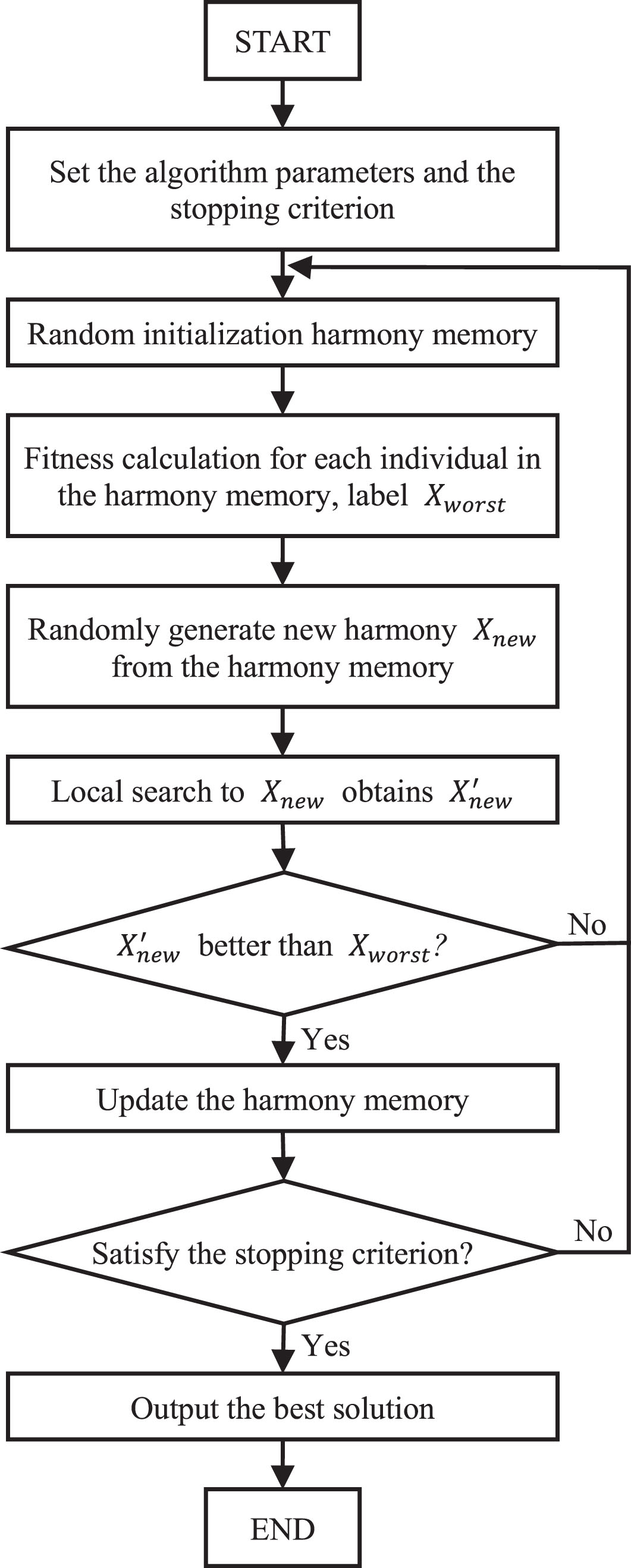
The flow chart of HSLS.

4.1.1 Coding

FJSP encode consists of machine coding and operation coding. The FJSP coding can be represented as a feasible solution using integer coding. The machine coding consists of integers of length l equal to the total number of operations, with each integer representing the number of machines on which the corresponding operation is processed. For example, in the P-FJSP example in Table 1, the job has seven operations, so the machine coding consists of integers of length seven [3 2 2 1 3 1 1]. The first integer 3 means that job 1 picks the fifth machine from the candidate machine set m∈ { m₁, m₂, m₅ } to be processed instead of m₃, and so on. The operation coding also consists of integer of length l, each representing the corresponding job number. For example, the operation coding of the P-FJSP example in Table 1 [2 3 1 2 1 3 1]. Job 1 has three operations so it happens exactly three times. The first integer 2 means that the first operation of job 2 is processed first, and the second integer 2 means the second operation of job 2 is processed. And so on. Finally, machine coding and operation coding are combined to represent a solution, such as [3 2 2 1 3 1 1 2 3 1 2 1 3 1].

4.1.2 Decoding

For ease of computation and understanding, the evolved individual encodings need to be decoded into practically feasible scheduling schemes. Using the decoding algorithm proposed in the paper by Shi et al [42] paper, the previously mentioned encodings are decoded as (2 1 2 2 0 2; 3 1 3 4 0 4; 1 1 5 5 0 5; 2 2 4 5 2 7; 1 2 3 2 5 7; 3 2 1 7 4 11; 1 3 4 9 7 16). The decoding method will not be described repeatedly here. The reader is referred to [40, 42] for a detailed description.

4.1.3 Variables chosen

The initial harmony vector generates a new harmony vector based on three rules: HMCR, PAR and random selection $X_{new} = {X_{1}^{new}, X_{2}^{new}, X_{3}^{new}, \dots, X_{HMS}^{new}}$ . First, $x_{i}^{new} (i = 1, 2, 3, \dots, HMS)$ is generated by HMCR and random selection. $x_{i}^{new} = {\begin{matrix} x_{i}^{new} \in x_{i}^{1, \dots, HMS}, r_{1} < HMCR \\ x_{i}^{new} \in X_{i}, other \end{matrix}$ (6) where r₁ ∈ [0, 1] the random number.

If, $x_{i}^{new}$ takes the value HM, then Pitch adjusting is performed on $x_{i}^{new}$ , i.e. $x_{i}^{new} = {\begin{matrix} x_{i}^{new} \pm B, r_{2} < PAR \\ x_{i}^{new}, other \end{matrix}$ (7) where r₂ ∈ [0, 1] the random number. B adjusts the bandwidth for the tone.

4.2 Local search

a) Insertion, swap and reverse operators [14]

These three operators are frequently used in local search. Insertion is the random insertion of an operation from its current location to other locations in a sequence of operations. If the insertion is backward, the operation between the start points and the insertion point moves forward; otherwise, it moves backward. Swap is used to randomly swap the locations of two operations. Reverse is to reverse the order of operations between two randomly selected points.

b) Tabu search [36]

TB is a global stepwise optimization algorithm. Tabu table is used to label the researched neighborhood and local optimal point, and the repeated search of the searched area in tabu table is avoided in the next search, which is beneficial to expand the search space to find the global optimal solution.

TB mainly considers tabu object, tabu length, number of candidate solution set, amnesty condition and termination rule. Tabu length is a very important parameter, which directly affects the search process and behavior of the whole algorithm. The size of candidate solution set refers to the number of candidate neighborhood solution. Termination iteration size refers to the number of tabu searches.

c) Simulated annealing [6]

SA is a global optimization algorithm that converges to the global optimal solution with probability, which is derived from the solid annealing principle. SA mainly includes two parts, metropolis criterion and annealing process. When the particle is at temperature T, with time, the temperature is continuously reduced according to the attenuation factor until the critical value is reached. According to the metropolis criterion, a new solution with a certain probability of exp(- Δt′/T) is accepted. Where Δt′ represents the difference between the new objective value and the previous one.

d) Variable neighborhood search [34]

VNS is a general framework to solve optimization problems. The basic idea is to use different neighborhood structures to search. First, search in the smallest neighborhood. When the optimal solution cannot be improved, search in a slightly larger neighborhood. If the optimal solution is improved, it will return to the smallest neighborhood structure to continue the search, otherwise, it will continue to replace the larger neighborhood structure to search. And so on until the termination condition is met.

The first level of the neighborhood structure operates only on machine codes. A process is randomly selected and the processing machine of the process is replaced by the machine with the shortest processing time. The second level of neighborhood structure operates only on job codes. A process is randomly selected and the process is interchanged with the head or tail of the process. The third level of neighborhood structure operates on both machine and job codes. Two processes are randomly selected to be interchanged and the machine is changed accordingly.

4.3 Evaluation index

It proposes for solving the FJSP with the criterion to deviation rate (D_r). Deviation rate can be expressed by the following formula. $D_{r} = \frac{\sum_{i}^{n = 50} (V_{i} - V_{m})}{n} \times 100 %$ (8) where V_i is the optimal value found, V_m refers to the best solution found in the literature so far, and n is the number of independent runs.

5 Experimental results and discussions

Firstly, how the HMS, HMCR and PAR affect the performance of HSLSs with a given number of decodes is investigated. Secondly, the effect of L_r and L_i on the performance of HSLSs is discussed. Finally, the optimal parameter and local search combinations are chosen to solve more FJSP examples to verify the effectiveness of HSLS in solving FJSP.

5.1 Effect of harmony memory size on HSLSs

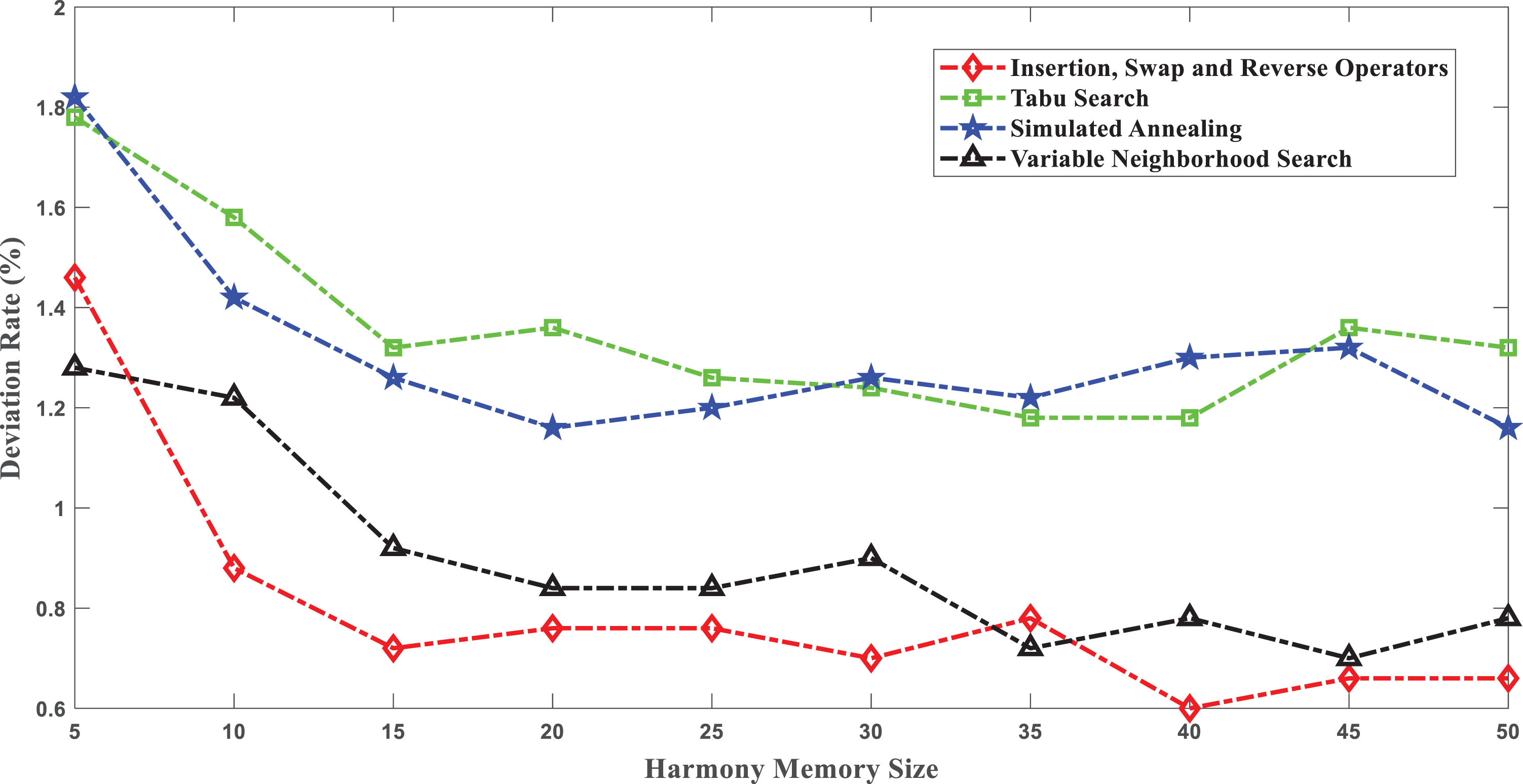
The MK01 instance (10 × 10 FJSP) mentioned in Brandimart [28] was used to study the effect of the harmony memory size on HSLSs. This instance, which has a reasonable number of machines and jobs and moderate difficulty, has been extensively studied in several studies (Yuan et al. [46]; Gao et al. [19]; Kong et al. [38]). The tabu search length (TB) was set to 13 and the number of candidate solution sets was set to 20. The initial temperature of SA was set equal to the total number of processes and the decay factor was set to 0.3. To ensure that the four local searches were investigated with the same number of decodes, the number of decodes was set to a larger number of 500,000. The other parameters were set as follows: HMCR = 0.9, PAR = 0.05, L_r = 0.2, L_i = 1000, HMS varies from 5 to 50 with a step size of 5. Each algorithm is run 50 times independently and the performance of the HSLSs is measured by D_r. The simulation results are shown in Fig. 2.

Fig. 2

Effect of harmony memory size on HSLSs.

In Fig. 2, the X-axis and Y-axis represent HMS and D_r respectively. When HMS is 5, the D_r of the four local searches is the largest, and the performance of the HSLSs is extremely poor. No optimal value of 40 can be found (the optimal value of MK01 FJSP is 40, and Fig. 3 shows its Gantt chart). As the HMS increases to 15, the performance of the HSLSs improves rapidly. However, as the HMS continues to increase, the performance of the HSLSs slowly decreases and levels off. When HMS = 40, the minimum D_r of HSLS-TB is 1.18. When HMS = 50, HSLS-SA has a minimum D_r of 1.16. If HMS = 45, the minimum D_r of HSLS-VNS is 0.7. When HMS = 40, the minimum D_r of HSLS-ISR is 0.6. HSLS-ISR and HSLS-VNS perform significantly better than HSLS-TB and HSLS-SA. The best performance is achieved with HSLS-ISR. To obtain HSLSs with good performance, the value of HMS should be large, but not too large. In general, values should be in the range of 15 to 40.

Fig. 3

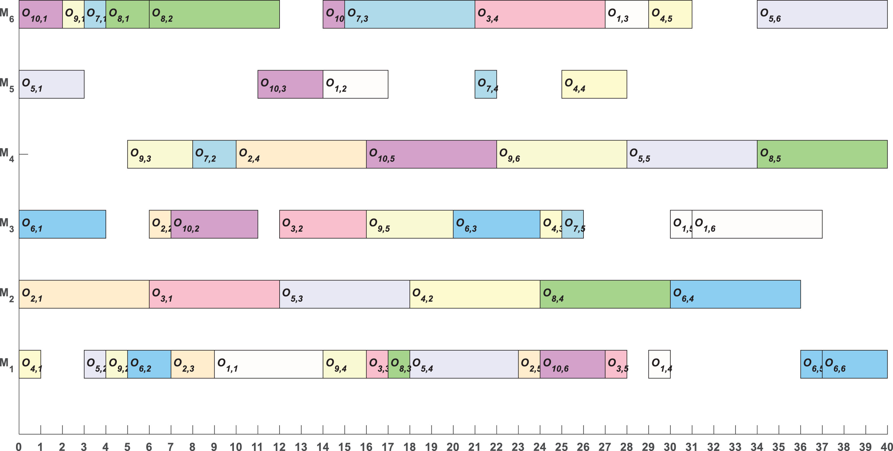
Gantt chart of a solution to MK01.

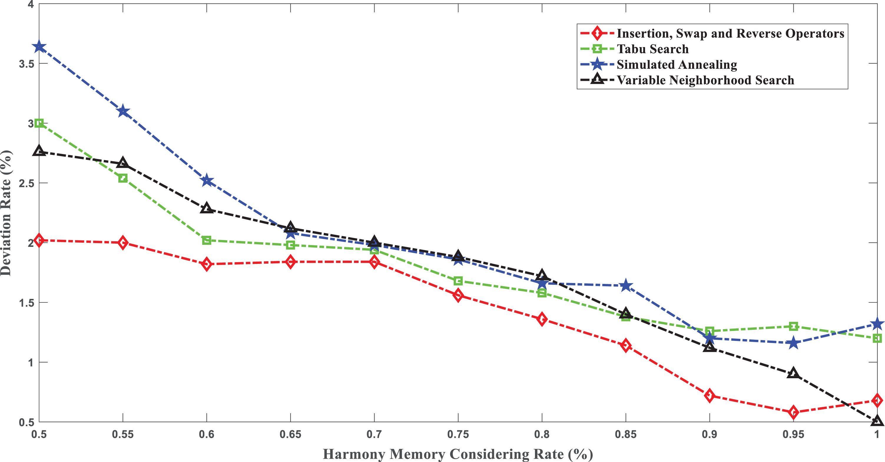
5.2 Effect of harmony memory considering rate on HSLSs

The MK01 example is used again. First, the effect of HMCR on HSLS performance was investigated. The HMCR varies from 0.5 to 1 in steps of 0.05. Based on the study in Section 5.1, HM = 40 is used in the following study. The other parameters are the same as those chosen in Section 5.1. The simulation results are shown in Fig. 4.

Fig. 4

Effect of harmony memory considering rate on HSLSs.

In Fig. 4. When HMCR = 0.5, the D_r values of the four local searches are the largest, and HSLSs also has the worst performance. Can’t find the optimal solution 40. As the HMCR increases, the performance of HSLSs improves. When HMCR = 0.95, the D_r of HSLS-ISR and HSLS-SA are 0.58 and 1.16 respectively. When HMCR = 1, the D_r of HSLS-TB and HSLS-VNS are 1.2 and 0.5 respectively. The minimum D_r of HSLS-VNS is lower than that of HSLS-ISR, but the overall performance of HSLS-ISR is better than the other three. Therefore, for a given number of decoding times, the performance of HSLSs increases as the HMCR increases. To obtain HSLSs with good performance, the value of HMCR should be as close to 1 as possible rather than equal to 1. In general, the range of values should be [0.9, 0.95].

5.3 Effect of pith adjusting rate on HSLSs

The MK01 FJSP instance mentioned above is used again. The effect of PAR on HSLS performance was investigated. The PAR was varied from 0 to 0.5 in steps of 0.05. Based on the study in Section 5.2, HMCR = 0.95 is used in the following study. The other parameters are the same as those selected in Section 5.2. The simulation results are shown in Fig. 5.

Fig. 5

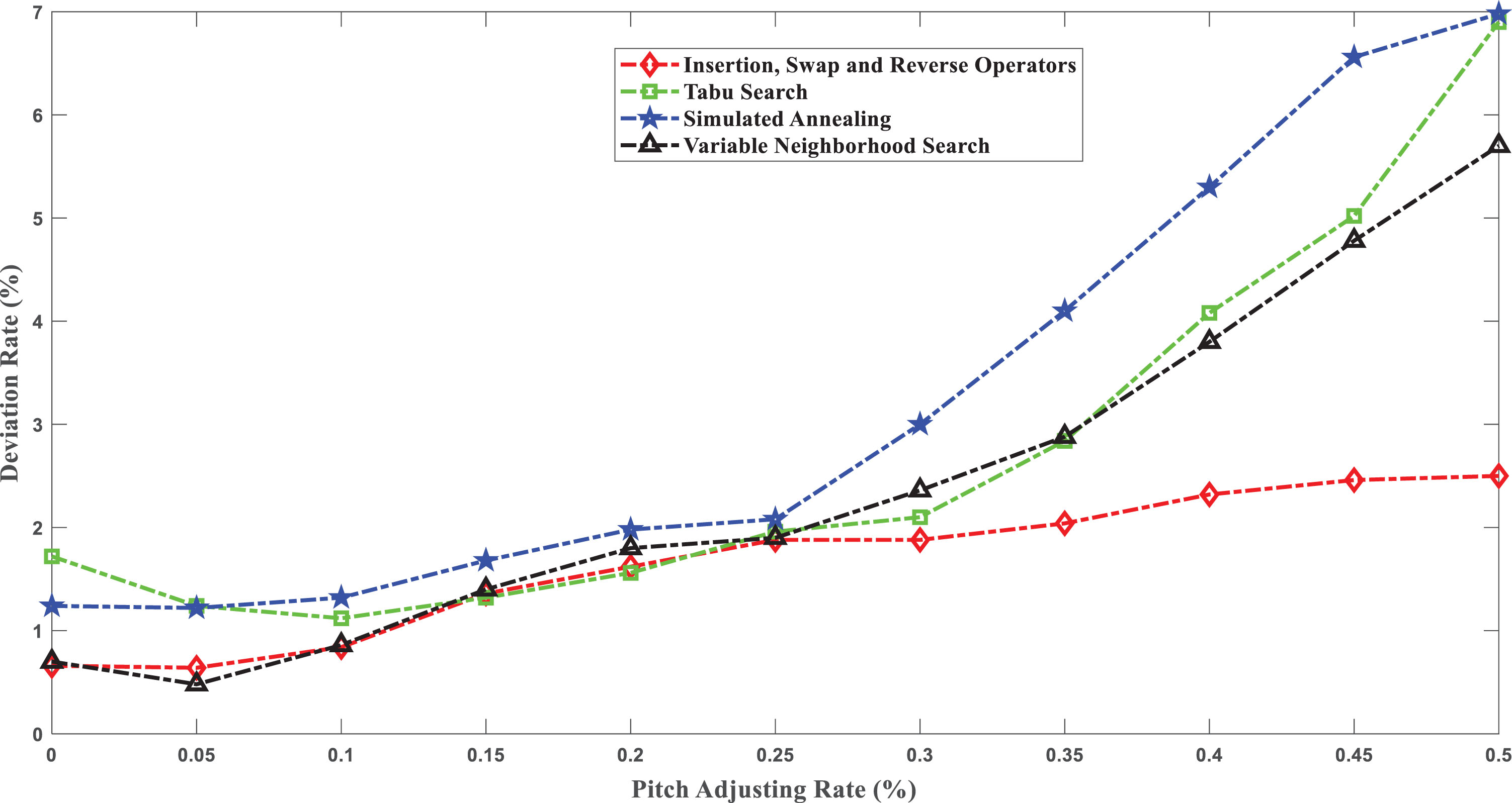
Effect of pith adjusting rate on HSLSs.

When PAR = 0.05, HSLS-ISR, HSLS-SA and HSLS-VNS achieve the best performance with D_r values of 0.64, 1.22 and 0.48 respectively. The best performance of HSLS-TB is achieved with PAR = 0.1 and D_r = 1.12. As PAR increases, the D_r of the four local searches also increases, and the performance of the HSLSs deteriorates slowly and then rapidly. When PAR = 0.5, the D_r of HSLS-TB and HSLS-SA are 6.9 and 6.98 respectively, at which point it is difficult for both to find the optimal solution. When PAR is between 0.05 and 0.25, the performance of the HSLSs is almost the same, but when PAR is greater than 0.25, HSLS-ISR performs significantly better than the other three. In general, the performance of HSLSs is better when the value of PAR is smaller, but the value of PAR should not be 0. In general, the value range should be [0.05, 0.1].

5.4 Effect of local search frequency on HSLSs

The MK01 FJSP example was used again to investigate the effect of local search frequency L_r on HSLSs performance. L_r was varied between 0.1 and 1 in steps of 0.1. Based on the study in Section 5.3, PAR = 0.05 is used in the following study. The remaining parameters are the same as those selected in Section 5.3. The simulation results are shown in Fig. 6.

Fig. 6

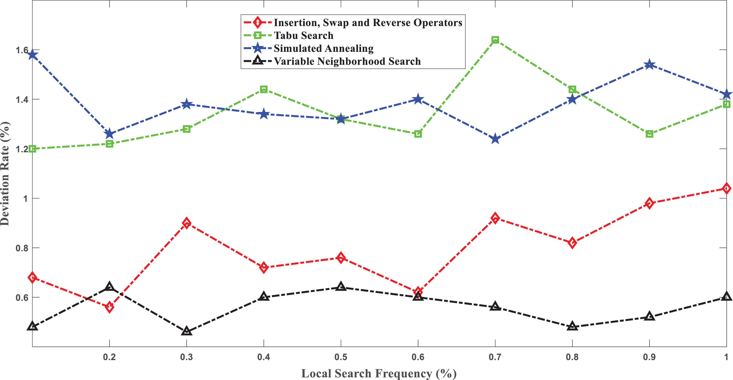
Effect of local search frequency on HSLSs.

When L_r is 0.2 and 1, the D_r of HSLS-ISR is 0.56 and 1.04 respectively. And the performance of HSLS-ISR is best and worst, respectively. When L_r is 0.1 and 0.7, the D_r of HSLS-TB and HSLS-SA are 1.2 and 1.24 respectively, which is the best performance of the two, but the optimal solution is still not found 40. The performance of HSLS-ISR and HSLS-VNS is significantly better than that of HSLS-TB and HSLS-SA. Only when L_r = 0.2 the performance of HSLS-ISR better than that of HSLS-VNS, with D_r of 0.56 and 0.64 respectively. However, the overall performance of HSLS-VNS is better than that of HSLS-ISR, not the reverse. As L_r increases, D_r first becomes small, then flattens out and then becomes large. In general, the value of L_r should be between 0.2 and 0.7 for the same number of decoding times.

5.5 Effect of local search intensity on HSLSs

The MK01 FJSP example was used again to investigated the effect of the local search intensity L_i on HSLSs performance. The L_i was varied between 500 and 1,500 in steps of 100. Based on the study in Section 5.4, the following study takes L_r = 0.2. The remaining parameters are the same as those selected in Section 5.4. The simulation results are show in Fig. 7.

Fig. 7

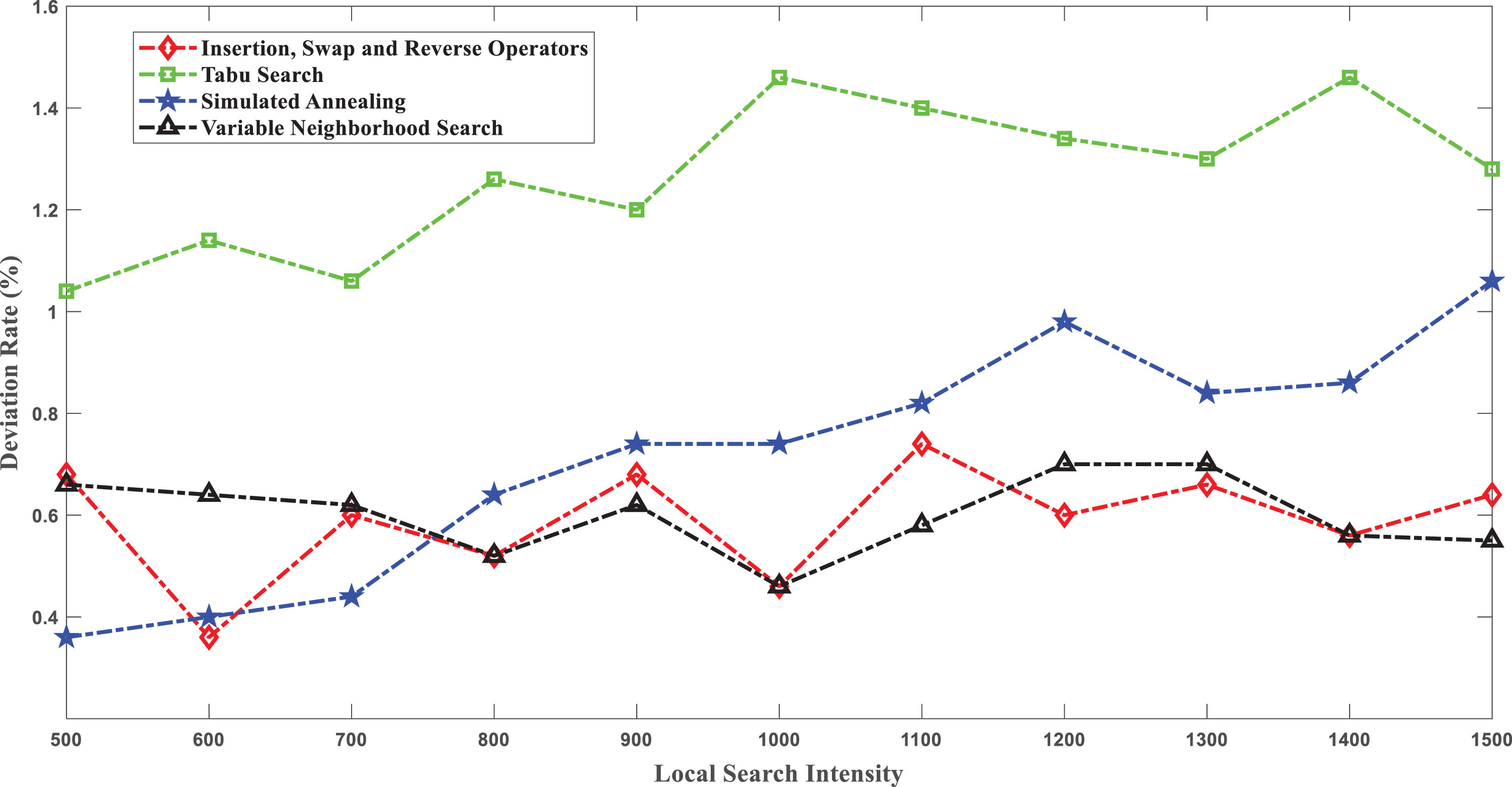
Effect of local search intensity on HSLSs.

When L_i is 500 and 600, the D_r of both HSLS-TB and HSLS-ISR is 0.36, at which point the HSLSs perform best and both can find the optimum value of 40. As L_i increases, the performance of HSLSs decreases continuously, after which the performance fluctuates continuously up and down, HSLS-TB and HSLS-SA have the best performance at L_i = 500, with D_r of 1.04 and 0.36 respectively. At L_i = 1000 and 1400, HSLS-ISR and HSLS-VNS have the same performance and D_r is the same 0.46 and 0.56. HSLS-TB has the worst performance of the three, followed by HSLS-SA. In general, the higher the L_i, the worse the performance of the HSLSs. In general, the range of values should be [500, 1000].

5.6 Comparison of local search algorithms

The optimal parameters of each local search are obtained through the above experiments, and the comparative analysis of the algorithms is carried out through K-data and F-data. The results of the experimental comparison are shown in Table 2. As can be seen from Table 2, for small instances SFJS01∼10,

Table 2
Comparison results of local search algorithms

Problems	HSLS-ISR	HSLS-TB	HSLS-SA	HSLS-VNS
8 × 8	14	15	15	14
10 × 10	7	8	7	8
15 × 10	11	15	14	12
SFJS01	66	66	66	66
SFJS02	107	107	107	107
SFJS03	221	221	221	221
SFJS04	355	355	355	355
SFJS05	119	119	119	119
SFJS06	320	320	320	320
SFJS07	397	397	397	397
SFJS08	253	253	253	253
SFJS09	210	210	210	210
SFJS10	516	516	516	516
MFJS01	468	468	468	468
MFJS02	448	460	448	465
MFJS03	466	468	468	469
MFJS04	564	568	564	571
MFJS05	514	539	514	514
MFJS06	634	634	645	649
MFJS07	879	881	909	890
MFJS08	884	891	911	884

the four local search algorithms can find the optimal value. For medium and large instances MFJS07, the local search ISR can obtain the optimal value 879, while TB can only obtain the suboptimal value 881, and the worst value obtained by SA is 909. For 15x10 examples, the local search ISR can obtain the optimal value 11, while the other three local searches cannot obtain the optimal value 11, which shows that the local search ISR has the best performance when solving large examples.

5.7 Effectiveness of HSLS in solving FJSP

To further prove the correctness of the parameters of the proposed algorithm. In this study FJSPs were solved and compared with other algorithms (Kacem et al. [11]; Xia and Wu [37]; Bagheri et al. [1]; Demir and İşleyen [44]; Xie et al. [13]; Yuan et al. [46]). The FJSP instance data are Kacem data [11] and F-data [30]. Local search selects ISR. The algorithm parameters are: HM = 40, HMCR = 0.95, PAR = 0.05, L_r = 0.2 and L_i = 600. Tables 3 and 4 show the results, with the symbol “N/A” indicating that the author of the original text did not provide the corresponding data.

Table 3
Results of comparison with other algorithms on K-data

Problems AL + CGA PSO + SA AIA HSLS-ISR

8 × 8 15 15 14 14

10 × 10 7 7 7 7

15 × 10 24 12 11 11

Problems	AL + CGA	PSO + SA	AIA	HSLS-ISR
8 × 8	15	15	14	14
10 × 10	7	7	7	7
15 × 10	24	12	11	11

Table 4

Results of comparison with other algorithms on F-data

Problems	M2	HA	HHS	AIA	HSLS-ISR
SFJS01	66	66	66	66	66
SFJS02	107	107	107	107	107
SFJS03	221	221	221	221	221
SFJS04	355	355	355	355	355
SFJS05	119	119	119	119	119
SFJS06	320	320	320	320	320
SFJS07	397	397	397	397	397
SFJS08	253	253	253	253	253
SFJS09	210	210	210	210	210
SFJS10	516	516	516	516	516
MFJS01	468	468	468	468	468
MFJS02	446	446	446	448	448
MFJS03	466	466	466	468	466
MFJS04	564	554	564	554	564
MFJS05	514	514	514	527	514
MFJS06	634	634	634	636	634
MFJS07	928	879	879	879	879
MFJS08	N/A	884	884	884	884

As shown in Table 3, when 8 × 8 is solved by HSLS-ISR, the optimal solution is 14, which is better than 15 of the “AL+CGA” algorithm. When 15 × 10 is solved, it is better than 12 of “PSO+SA”. When solving MFJS05 with HSLS-ISR, the optimal value is 514, which is better than 527 of AIA algorithm. When solving MFJS07 with HSLS-ISR, the optimal solution is 879, which is better than 928 of M2 algorithm. Figure 8 is a Gantt chart of the solution of the 15 × 10 problems.

Fig. 8

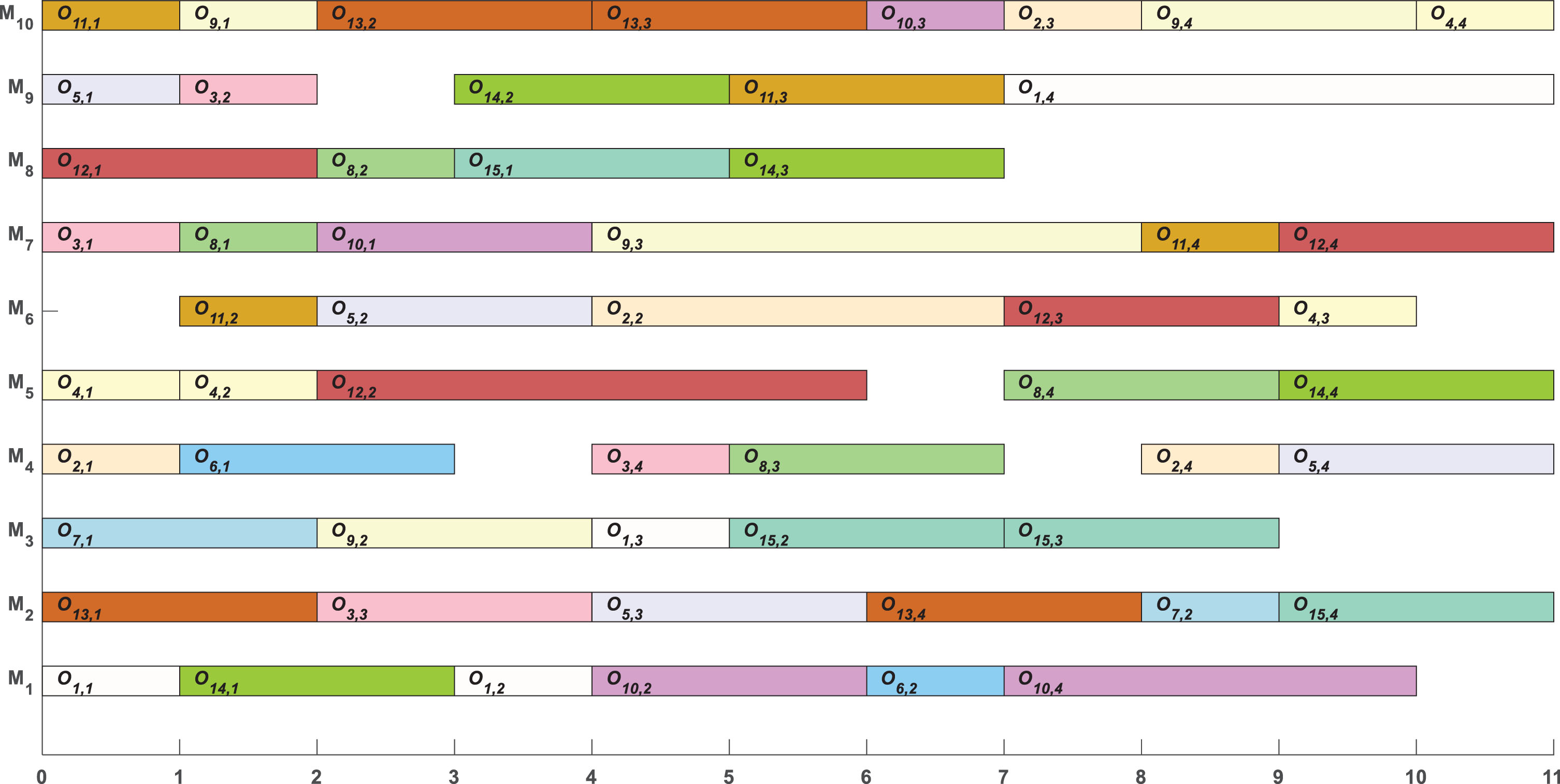
Gantt chart of a solution to 15 × 10.

5.8 Discussion

As mentioned in Section 5.1, for a certain number of decoding times, the performance of HSLSs increases with HMS, and the ability to find the global optimal solution becomes stronger. However, as the HMS increases, so does the amount of computation, which affects the speed of the final search for the optimal solution, and performance is reduced. So bigger is not always better.

As mentioned in Sections 5.2 and 5.3. As HMCR increases, the overall trend of D_r is downward, and the performance of HSLSs is constantly improving. In generally, the performance of HSLSs is optimal when HMCR is 0.95 rather than 1. PAR and HMCR have the opposite trend. As PAR increases, the performance of HSLS-TB, HSLS-SA and HSLS-VNS decreases slowly and then rapidly. However, the performance of HSLS-ISR decreases slowly. The optimum performance of the HSLSs is all concentrated at PAR = 0.05 instead of 0. The values of HMCR and PAR can be set to sum to 1.

As mentioned in Sections 5.4 and 5.5, the performance of the HSLSs varies continuously with different L_r. The overall performance of HSLS-ISR and HSLS-VNS is better than that of HSLS-TB and HSLS-SA. The performance of HSLS-ISR is better than that of HSLS-VNS only when L_r is 0.2, but the overall performance of HSLS-VNS is better than that of HSLS-ISR. HSLS-VNS can find the optimal value 40 for L_r values between 0 and 1. As the local search intensity increases, the performance of HSLSs first improves and then deteriorates towards continuous variation. The smallest D_r of HSLS-TB is 1.04 for L_i = 500, and none of the optimal solutions can be found at 40. The largest D_r of HSLS-VNS is 0.7 for L_i = 4000 and the optimal solution can be found in almost all cases 40. HSLS-SA, HSLS-ISR and HSLS-VNS have similar overall performance, but are better than HSLS-TB.

6 Conclusion and future work

In this study, four commonly used local search algorithms were combined with HS to obtain HSLSs. At a certain number of decoding times, HSLSs were used to solve the MK01 FJSP instance, and the influence of parameters such as HMS, HMCR, PAR, L_r and L_i on HSLSs was systematically investigated. The simulation results showed that the combination of harmony search and local search can significantly improve the performance compared with the standard HS, and the performance of different local searches is also different. For HMS, the parameter should be larger, but the performance will degrade if it is too large, and the expectation interval is [15, 40]. The opposite is true for HMCR and PAR. HMCR should be as close to 1 as possible, but it cannot be 1. PAR should be as close to 0 as possible. The best value is 0.05 and the sum of these two values is 1. For L_r the expected value is in [0.2, 0.7]. The expected value of L_i is in the range [500, 1,000]. Overall, HSLS-ISR and HSLS-VNS perform better than HSLS-TB and HSLS-SA, with HSLS-ISR performing best. The results of the study can help researchers understand how to achieve better HSLSs using local search.

In this study, multiple local search algorithms combined with standard harmony search algorithms were used to obtain HSLSs. However, this may limit its performance and only solves small FJSPs. In the future, adaptive parameters and improvements to the local search structure will be considered to better address larger scale FJSPs.

Conflicts of interest

The authors declare no conflicts of interest regarding the publication of this paper.

Footnotes

Acknowledgments

This research is partially supported by the Natural Science Foundation of Sichuan Province (Grant No. 2023NSFSC0507), the Program for HUST State Key Laboratory of Intelligent Manufacturing Equipment and Technology (Grant No. IMETKF2023026), the Key Laboratory of Icing and Anti/De-icing of CARDC (Grant No. IADL20220405), and the Natural Science Foundation of Southwest University of Science and Technology (Grant No. 20zx7117).

References

Bagheri

, Zandieh

, Mahdavi

and Yazdani

, An artificial immune algorithm for the flexible job-shop scheduling problem, Future Generation Computer Systems 26(4) (2010), 533–541.

Destouet

, Tlahig

, Bettayeb

and Mazari

, Flexible job shop scheduling problem under industry 5.0: a survey on human reintegration, environmental consideration and resilience improvement, Journal of Manufacturing Systems 67 (2023), 155–173.

Soto

, Dorronsoro

, Fraire

, Cruz-Reyes

, Gomez-Santillan

and Rangel

, Solving the multi-objective flexible job shop scheduling problem with a novel parallel branch and bound algorithm, Swarm and Evolutionary Computation 53 (2020), 100632.

Hoitomt

D.J.

, Luh

P.B.

and Pattipati

K.R.

, A practical approach to job-shop scheduling problems,Transactions, on Robotics and Automation 9(1) (1993), 1–13.

Abd

E.M.A.E.

, Mohamed

S.A.O.

and Mohamed

B.A.H.

, Optimality of the flexible job shop scheduling problem, African Journal of Mathematics and Computer Science Research 4(10) (2011), 321–328.

Defersha

F.M.

, Obimuyiwa

and Yimer

A.D.

, Mathematical model andsimulated annealing algorithm for setup operator constrainedflexible job shop scheduling problem, Computers & Industrial Engineering 171 (2022), 108487.

Zhang

, Gao

and Shi

, An effective genetic algorithm for the flexible job-shop scheduling problem, Expert Systems with Applications 38(4) (2011), 3563–3573.

Zhang

, Zhang

, Song

, Wang

and Zhou

, A variable neighborhood search based genetic algorithm for flexible job shop scheduling problem, Cluster Computing 22 (2019), 11561–11572.

Zhang

, Hu

, Sun

and Zhang

, An improved genetic algorithm for the flexible job shop scheduling problem with multiple time constraints, Swarm and Evolutionary Computation 54 (2020), 100664.

10.

, Sun

, Chen

and Liang

, An efficient artificial fish swarm model with estimation of distribution for flexible job shop scheduling, International Journal of Computational Intelligence Systems 9(5) (2016), 917–931.

11.

Kacem

, Hammadi

and Borne

, Approach by localization and multi-objective evolutionary optimization for flexible job-shop scheduling problems, IEEE Transactions on Systems, Man, and Cybernetics, Part C (Applications and Reviews) 32(1) (2002), 1–13.

12.

Fan

, Shen

, Gao

, Zhang

and Zhang

, A hybrid Jaya algorithm for solving flexible job shop scheduling problem considering multiple critical paths, Journal of Manufacturing Systems. 60 (2021), 298–311.

13.

Xie

, Gao

, Peng

, Li

and Li

, Review on flexible job shop scheduling, IET Collaborative Intelligent Manufacturing 1(3) (2019), 67–77.

14.

J.Q.

, Pan

Q.K.

and Gao

K.Z.

, Pareto-based discrete artificial bee colony algorithm for multi-objective flexible job shop scheduling problems, The International Journal of Advanced Manufacturing Technology 55 (2011), 1159–1169.

15.

J.Q.

, Pan

Q.K.

and Liang

Y.C.

, An effective hybrid tabu searchalgorithm for multi-objective flexible job-shop scheduling problems, Computers & Industrial Engineering 59(4) (2010), 647–662.

16.

Gao

, Yang

, Zhou

, Pan

and Suganthan

P.N.

, Flexible job-shop rescheduling for new job insertion by using discrete Jaya algorithm, IEEE transactions on cybernetics 49(5) (2019), 1944–1955.

17.

Gao

, Cao

, Zhang

, Chen

, Han

and Pan

, A review on swarm intelligence and evolutionary algorithms for solving flexible job shop scheduling problems, IEEE/CAA Journal of Automatica Sinica 6(4) (2019), 904–916.

18.

Gao

K.Z.

, Suganthan

P.N.

and Chua

T.J.

, Pareto-based discrete harmony search algorithm for flexible job shop scheduling, In 2012 12th International Conference on Intelligent Systems Design and Applications (ISDA) 11 (2012), 953–956.

19.

Gao

K.Z.

, Suganthan

P.N.

, Pan

Q.K.

, Chua

T.J.

, Cai

T.X.

and Chong

C.S.

, Discrete harmony search algorithm for flexible job shop scheduling problem with multiple objectives, Journal of Intelligent Manufacturing 27 (2016), 363–374.

20.

Gao

K.Z.

, Suganthan

P.N.

, Pan

Q.K.

, Chua

T.J.

, Cai

T.X.

and Chong

C.S.

, Pareto-based grouping discrete harmony search algorithm for multi-objective flexible job shop scheduling, Information Sciences 289 (2016), 76–90.

21.

Wang

, Cai

, Li

, Liu

Flexible job shop scheduling problem using an improved ant colony optimization, Scientific Programming (2017), 2017.

22.

Wang

, Yang

, Xu

, Niu

, Pardalos

P.M.

and Fei

, An improved adaptive binary harmony search algorithm, Information Sciences 232 (2013), 58–87.

23.

, Sun

and Ming

, Flexible job shop scheduling based on multi-population genetic-variable neighborhood search algorithm, In 2015 4th International Conference on Computer Science and Network Technology (ICCSNT) 9(1) (2015), 244–248.

24.

Hajibabaei

and Behnamian

, Fuzzy cleaner production in assembly flexible job-shop scheduling with machine breakdown and batch transportation: Lagrangian relaxation, Journal of Combinatorial Optimization 45(5) (2023), 112.

25.

Huang

, Wang

L.M.

and Liang

, An improved adaptive genetic algorithm in flexible job shop scheduling, In 2016 2nd International Conference on Cloud Computing and Internet of Things (CCIOT) 10 (2016), 177–184.

26.

Bragin

M.A.

, Survey on Lagrangian relaxation for MILP: importance, challenges, historical review, recent advancements, and opportunities, Annals of Operations Research (2023), 1–17.

27.

Gomes

M.C.

, Barbosa-Póvoa

A.P.

and Novais

A.Q.

, Reactive scheduling in a make-to-order flexible job shop with re-entrant process and assembly: a mathematical programming approach, International Journal of Production Research 51(17) (2013), 5120–5141.

28.

Brandimarte

, Routing and scheduling in a flexible job shop by tabu search, Annals of Operations Research 41(3) (1993), 157–183.

29.

Brucker

and Schlie

, Job-shop scheduling with multipurpose machines, Computing (1990).

30.

Fattahi

, Mehrabad

M.S.

and Jolai

, Mathematical modeling and heuristic approaches to flexible job shop scheduling problems, Journal of Intelligent Manufacturing 18 (2007), 331–342.

31.

Chen

, Yang

, Li

and Wang

, A self-learning geneticalgorithm based on reinforcement learning for flexible job-shopscheduling problem, Computers & Industrial Engineering 149 (2020), 106778.

32.

Zhang

and Wu

, A hybrid immune simulated annealing algorithm for the job shop scheduling problem, Applied Soft Computing 10(1) (2010), 79–89.

33.

Caldeira

R.H.

and Gnanavelbabu

, Solving the flexible job shopscheduling problem using an improved Jaya algorithm, Computers& Industrial Engineering 137 (2019), 106064.

34.

Jun

, Lee

and Chun

, Learning dispatching rules using random forest in flexible job shop scheduling problems, International Journal of Production Research 57(10) (2019), 3290–3310.

35.

Lloyd

, Yu

and Konstas

, FMS scheduling using Petri net modeling and a branch & bound search. In Proceedings, IEEE International Symposium on Assembly and Task Planning 8 (1995), 141–146.

36.

Mahmud

, Abbasi

, Chakrabortty

R.K.

and Ryan

M.J.

, Multi-operator communication based differential evolution with sequential Tabu Search approach for job shop scheduling problems, Applied Soft Computing 108 (2021), 107470.

37.

Xia

and Wu

, An effective hybrid optimization approach formulti-objective flexible job-shop scheduling problems, Computers & Industrial Engineering 48(2) (2005), 409–425.

38.

Kong

, Yao

, Yang

and Su

, Solving the flexible job shop scheduling problem using a discrete improved grey wolf optimization algorithm, Machines 10(11) (2022), 1100.

39.

and Gao

, An effective hybrid genetic algorithm and tabu search for flexible job shop scheduling problem, International Journal of Production Economics 174 (2016), 93–110.

40.

Shi

, Long

, Li

and Deng

, Multi-population genetic algorithm with ER network for solving flexible job shop scheduling problems, PloS One 15(5) (2020), e0233759.

41.

and Li

, Two layered approaches integrating harmony searchwith genetic algorithm for the integrated process planning andscheduling problem, Computers & Industrial Engineering 155 (2021), 107194.

42.

Shi

X.Q.

, Long

, Li

Y.Y.

, Wei

Y.L.

and Deng

D.S.

, Different performances of different intelligent algorithms for solving FJSP: a perspective of structure, Computational Intelligence and Neuroscience 2018 (2018).

43.

, Chen

, Gao

, Li

and Zhang

, Multi-objective flexible job-shop rescheduling with new job insertion and machine preventive maintenance, IEEE Transactions on Cybernetics 5(53) (2023), 3101–3113.

44.

Demir

and İşleyen,

S.K.

, Evaluation of mathematical modelsfor flexible job-shop scheduling problems. Applied, MathematicalModelling 37(3) (2013), 977–988.

45.

, Huang

, Wu

and Guo

, An improved artificial bee colony algorithm for solving multi-objective low-carbon flexible job shop scheduling problem, Applied Soft Computing 95 (2020), 106544.

46.

Yuan

, Xu

and Yang

, A hybrid harmony search algorithm for the flexible job shop scheduling problem, Applied soft computing 13(7) (2013), 3259–3272.

Research on the performance of harmony search with local search algorithms for solving flexible job-shop scheduling problem

Abstract

Keywords

1 Introduction

2 Literature review

3 Flexible job-shop scheduling problem

Table 1 An instance of P-FJSP Jobs Operations M 1 M 2 M 3 M 4 M 5 J 1 O 11 7 5 – – 5 O 12 3 – 2 – 7 O 13 – 4 – 9 2 J 2 O 21 – 2 6 – 5 O 22 4 4 – 5 9 J 3 O 31 – – 4 5 – O 32 7 – – 3 –

4.1 HSLS for solving FJSP

4.1.2 Decoding

4.1.3 Variables chosen

4.3 Evaluation index

5.1 Effect of harmony memory size on HSLSs

Table 2 Comparison results of local search algorithms

Table 3 Results of comparison with other algorithms on K-data Problems AL + CGA PSO + SA AIA HSLS-ISR 8 × 8 15 15 14 14 10 × 10 7 7 7 7 15 × 10 24 12 11 11

6 Conclusion and future work

Conflicts of interest

Footnotes

Acknowledgments

References

Table 1
An instance of P-FJSP

Jobs Operations M ₁ M ₂ M ₃ M ₄ M ₅

J ₁ O ₁₁ 7 5 – – 5

O ₁₂ 3 – 2 – 7

O ₁₃ – 4 – 9 2

J ₂ O ₂₁ – 2 6 – 5

O ₂₂ 4 4 – 5 9

J ₃ O ₃₁ – – 4 5 –

O ₃₂ 7 – – 3 –

Table 2
Comparison results of local search algorithms

Table 3
Results of comparison with other algorithms on K-data

Problems AL + CGA PSO + SA AIA HSLS-ISR

8 × 8 15 15 14 14

10 × 10 7 7 7 7

15 × 10 24 12 11 11