Engine misfire fault diagnosis based on SC

Abstract

Misfire fault is a common engine failure which is caused by incomplete combustion in the engine cylinders. Conventionally, the misfire fault is diagnosed manually by mechanics, but the diagnosis process is time-consuming. Therefore, this study aims to explore the feasibility of using Subtractive Clustering based Adaptive Neuro-Fuzzy Inference System (SC-ANFIS) algorithm to assist in diagnosing misfire faults. The Subtractive Clustering (SC) approach initializes the parameters of Adaptive Neuro-Fuzzy Inference System (ANFIS), whereas Back Propagation (BP) and Least Square Estimation (LSE) approaches are implemented to optimize the ANFIS parameters. The proposed algorithm will pre-diagnose the cause of misfire faults based on the engine exhaust gas. In this work, exhaust gases for different causes of misfire faults are collected from Volkswagen 1.8TSI 4-cylinder petrol engine. These collected data are used to train the proposed algorithm. The performances of the proposed algorithm are compared to two commonly used algorithms, namely Fuzzy C-Mean Clustering based ANFIS (FCM-ANFIS) and BP algorithms. The simulation results show the proposed algorithm has improved 2.4% to 5.5% averagely in terms of accuracy, efficiency and stability.

Keywords

Engine misfire fault diagnosis SC-ANFIS FCM-ANFIS

1 Introduction

Misfire faults are common engine failures when the air-fuel mixture in the cylinder cannot be combusted normally due to the failure in mechanical or electronic parts [1]. The failures may manifest as either single-cylinder or multi-cylinder misfires, and either intermitted or continuous misfires. For a multi-cylinder engine, misfire faults are difficult to detect as misfires vary in terms of severity, impact and difficulty in diagnosis under various conditions.

Misfire faults occur in most of vehicles in the market. It will cause serious consequences if it is not solved. The consequences of misfire can be categorized into three categories based on their severities:

If the misfire fault is not serious, the air-fuel mixture will not fully burn, and it resulted in inefficient fuel consumption that decreases the vehicular output power. A misfire fault can cause a loss of 0% to 100% of engine power [2].

If the misfire fault is serious, the engine will fail to burn the air-fuel mixture and eventually damage the three-way catalytic converter. This will lead to components in exhaust emissions exceeding the standard and cause serious air pollution. Based on statistical data [3, 4], when the engine cylinder misfire rate becomes 2%, the mobile exhaust pollutants will increase by 50% compared to the normal condition. In China, mobile exhaust pollution accounted for 70% of urban pollution in Shenzhen [5].

If the misfire fault is very serious, the engine will not work properly and eventually get damaged and even will pose safety issues to other road users. According to the World Health Organization (2018), 1.35 million people died in road traffic accidents in 2016. Road accident is the “number one killer” of children aged 5- to 14-year-old worldwide [6]. Based on the study of National Bureau of Statistics of China, there were 167,000 vehicular traffic accidents with 46,000 deaths in 2018 resulting in direct property losses of RMB 1.19 billion [7]. Vehicle malfunction is one of the main causes of traffic accidents [8].

Thus, it can be stated that misfire is a common vehicular failure that might result in serious consequences, such as loss of engine power, safety issue, air pollution, monetary loss [9]. Therefore, it is important to have a reliable, fast and accurate diagnosis system for engine misfire faults.

Engine misfire fault diagnosis is difficult to be conducted manually due to the lack of auxiliary equipment and diagnostic systems for engine monitoring. In common practice, On-Board Diagnostics (OBD) approach is implemented in engine misfire monitoring. However, the diagnostic capability of this approach is relatively low [10]. OBD can report fault codes for misfires, but it cannot diagnose the cause and degree of misfire faults. It has limited capability (70% to 80% only) in detecting faults in electronic control system [11].

Therefore, many studies had been conducted to seek for a reliable, efficiency and stable engine misfire fault diagnosis system. The misfire symptoms, such as exhaust gas composition [12], crankshaft speed [13], engine vibration [14], and integrating artificial intelligence (AI) in diagnosis approaches, such as Artificial Neural Network [15], Fuzzy Logic [16], and Support Vector Machine [17], were the main focus in those recent studies. However, the comprehensive performances of all the reported algorithms are inadequate in pre-diagnosing the misfire faults in terms of accuracy, efficiency and stability. This is because of the complex structure of engine, harsh working environment, uncertain and dynamic characteristics of misfire fault. Since misfire is highly-nonlinear, diagnosis becomes more challenges as it can be caused by multiple factors.

In order to overcome the inherent weakness of the reported algorithms, scholars tend to hybrid those algorithms [18]. Adaptive Neuro-Fuzzy Inference System (ANFIS) is one of the commonly reported algorithm for engine misfire diagnosis as it combines the advantages of both Artificial Neural Networks (has adaptive learning ability) and Fuzzy Logic (powerful in dealing uncertainty) [19]. With those advantages, ANFIS becomes a good candidate for fault diagnosis, pattern recognition, predictive systems, system identification, and non-linear control systems [20, 21]. However, traditional ANFIS has the disadvantages of being computationally intensive, slow to converge and a “dimensional disaster” [22, 23].

Thus, this work would like to improve the classical ANFIS by integrating Subtractive Clustering (SC) approach into it to form a SC-ANFIS algorithm. The proposed algorithm is trained using the collected experimental exhaust gas composition data under various misfire factors. The experiments were conducted using Volkswagen 1.8TSI 4-cylinder petrol engine as most of the on-road vehicles in China are using this model of engine. The aim of this work is to explore the feasibility of implementing SC-ANFIS to pre-diagnose engine misfire faults. The main contribution is the proposal to optimise the parameters of ANFIS using the generation and hybrid algorithms of the SC optimised initial fuzzy inference system. The construction of the SC-ANFIS engine misfire fault diagnosis platform improves the recognition speed, recognition rate and recognition stability of fault diagnosis. This provides a reference for academic research, a method for online diagnosis and prediction of misfire faults, and guidance and advice for maintenance engineers.

This paper is organized as follows: Section II critically reviews the engine misfire fault diagnosis approaches. Section III discusses the methodology of the proposed SC-ANFIS. Section IV presents the results and discuss the performances of the proposed algorithm. Section V concludes the findings of this work.

2 Literature review

Engine misfire is a hot topic in vehicle fault diagnosis research [24]. According to the relevant literature, currently, engine misfire fault diagnosis is carried out using the premise that the engine assembly is not disassembled or partially disassembled [25]. However, the engine is a complex system integrating different fields such as electronics, hydraulics, mechanics and electrics. The use of traditional fault diagnosis methods is clearly inadequate. The introduction of fault diagnosis methods of artificial intelligence into engine misfire fault diagnosis is a hot topic for research scholars.

Generally, the use of artificial intelligence for engine misfire fault diagnosis mainly consists of 2 parts, namely (1) fault sign information collection and (2) fault diagnosis methods. The engine fault sign information includes internal cylinder sign information and external cylinder sign information [26]. The fault diagnosis method includes single diagnosis method and comprehensive diagnosis method.

2.1 Fault diagnosis using signal information

In terms of diagnosis based on information from internal engine cylinder signs. The main internal cylinder signs for engine misfire diagnosis are ion current signals, optical signals, cylinder pressure, oil spectrum signs, thermal performance parameter signals, etc. Based on the cylinder internal signs information of misfire fault diagnosis, can be identified by direct measurement of the way misfire fault. This method is simple, reliable data, misfire fault diagnosis accuracy is high. However, the sensor quality requirements and manufacturing costs are high, and installation is very difficult. The market value of this method is limited and its practical significance is not significant [27].

In the area of diagnostics based on information from external engine cylinder signs. The external cylinder sign information for engine misfire diagnosis mainly includes crankshaft instantaneous angular velocity, crankshaft instantaneous angular acceleration, crankshaft instantaneous net torque, crankshaft angle, engine vibration signal, exhaust gas pressure, exhaust gas composition, exhaust gas temperature signal, exhaust gas noise, body noise signal, oxygen sensor signal, engine roughness, etc. Engine misfire fault diagnosis based on information from external cylinder signs is less expensive to implement and a simpler and easier process than information from internal cylinder signs. And the use of exhaust gas, vibration and crankshaft speed and other signs information, fast response, real-time better, can achieve online misfire fault diagnosis, the practice is more meaningful [12, 27].

Exhaust gas is an important external sign of an engine misfire. The essence of an engine misfire is whether the mixture in the cylinder is burning properly, and the engine exhaust is a product of the combustion of the mixture, so the engine exhaust composition can reflect the combustion situation very well. The volume fraction in engine exhaust gas varies under different misfire level fault conditions, and the content of HC, CO₂, CO, O₂, NO_X and other components in the exhaust gas can be used as engine misfire fault diagnosis sign information [28, 29]. Using the difference in volume fraction of each gas in engine exhaust gas composition to infer engine failure is an important trend in vehicle engine fault diagnosis [30].

The literature [12] points out that theoretical analysis and experimental evidence show that exhaust gas detection and analysis is an effective means of diagnosing engine faults. The exhaust gas composition is directly related to the engine operating conditions and can examine the combustion, ignition energy and mechanical conditions of the internal combustion engine. The use of exhaust gas sign information for engine misfire fault diagnosis is a mainstream direction of research.

2.2 Fault diagnosis using diagnostic methods

Typically, fault diagnosis methods are single diagnosis methods and integrated diagnosis methods. Common single diagnosis methods include Expert System (ES), Decision Fault Tree (DFT), Fuzzy Logic (FL), Artificial Neural Network (ANN), Support Vector Machine (SVM), Genetic Algorithm (GA), etc. Common integrated diagnostic methods include Fuzzy Expert System (FES), ANFIS, GA-SVM, etc. A single diagnostic method has characteristics and advantages in one aspect. Integrated diagnostic methods have characteristics and advantages in several aspects. Different diagnostic methods will vary in terms of where they are applicable due to their different characteristics and advantages.

FL and ANN are 2 important artificial intelligence techniques [31]. It has an important role for engine misfire fault diagnosis. This is because there are 2 very important characteristics of engine misfire faults and fault sign information. (1) Engine misfire faults are ambiguous in nature. (2) Engine misfire faults have a non-linear relationship with the main fault sign information. For the engine misfire fault characteristics (1), FL is most suitable because it is more reasonable to use fuzzy logic method for the diagnosis of engine misfire ambiguity. The literature [16] uses four engine misfire fault sign parameters for misfire diagnosis by fuzzy logic operations, and the results prove the scientific nature of this method. For engine misfire fault characteristics (2), ANN is most suitable as it is particularly suitable for dealing with non-linear problems [32]. The literature [15] and [33] demonstrate the feasibility and effectiveness of using ANN to diagnose engine misfire faults.

FL and ANN are two very potential methods for diagnosing engine misfire faults, but they are not ideal. This is because a single fault diagnosis theory and diagnostic technique is not a good solution to a practical problem [34]. FL can solve the fuzzy problem of engine misfire fault degree well, but it does not perform well on the dynamic problem of engine misfire fault with stochastic time-varying and uncertainties. However, ANN is outstanding in stochastic time-varying, uncertain and nonlinear dynamic problems, but ANN does not perform well in fuzzy problems and lacks explanatory power. At the same time, the engine is a closed-loop system composed of multiple systems. Engine misfire failure is an intricate problem. To solve the actual problem, we should not only focus on one aspect of the problem, but should consider the engine misfire failure problem comprehensively. A comprehensive intelligent diagnosis technology formed by integrating and complementing a variety of different fault diagnosis techniques or theories is an inevitable trend in the development of complex fault intelligent diagnosis technology [35]. Therefore, FL and ANN are combined to form fuzzy neural to improve the diagnostic performance of FL and ANN. There are many combinations of FL and ANN, among which ANFIS is a typical representative of the combination of FL and ANN. ANFIS has been proven to combine the advantages of ANN and FL, and has the advantages of strong adaptive learning ability, fast training speed, fast convergence speed and high prediction accuracy [20, 36]. It is suitable for dealing with ambiguity, uncertainty, time-varying, nonlinear dynamic problems [37]. Table 1 summarizes and compares FL, ANN, and ANFIS. Therefore, in theory ANFIS is well suited to handle engine misfire failures.

Table 1
Comparison of FL, ANN and ANFIS

Projects Technology FL ANN ANFIS

Structure Composition Fuzzy rule Neuron Fuzzy rule, Neuron

Knowledge Knowledge acquisition Expert knowledge Self-study Self-study

Knowledge representation membership function Distributed representation Distributed representation, membership function

reasoning Reasoning mechanisms Fuzzy rule combination Learn function calculations Fuzzy rule-based learning function calculations

Reasoning calculation Membership function calculation Neuronal superimposition Membership function calculation, Neuronal superimposition

Adaptive Learning mechanisms Summarization Adjustment of weights Adjustment of weights

Fault tolerance Low High High

Natural Language Achieving Explicit Not obvious Explicit

Flexibility High Low High

Uncertainty Information Quantity and quality Number Quantity and quality

Cognition Decision-making Perception Perception

Advantages and disadvantages Advantages Expert experience can be leveraged and reasoning is strong Strong self-learning and self-organisation skills Strong self-learning, self-organisation and reasoning skills. No a priori knowledge is required and automatic extraction of data features can be performed. Has interpretability.

Disadvantages Poor self-learning ability Black box model, difficult to express knowledge Single output

Projects	Technology	FL	ANN	ANFIS
Structure	Composition	Fuzzy rule	Neuron	Fuzzy rule, Neuron
Knowledge	Knowledge acquisition	Expert knowledge	Self-study	Self-study
	Knowledge representation	membership function	Distributed representation	Distributed representation, membership function
reasoning	Reasoning mechanisms	Fuzzy rule combination	Learn function calculations	Fuzzy rule-based learning function calculations
	Reasoning calculation	Membership function calculation	Neuronal superimposition	Membership function calculation, Neuronal superimposition
Adaptive	Learning mechanisms	Summarization	Adjustment of weights	Adjustment of weights
	Fault tolerance	Low	High	High
Natural Language	Achieving	Explicit	Not obvious	Explicit
	Flexibility	High	Low	High
Uncertainty	Information	Quantity and quality	Number	Quantity and quality
	Cognition	Decision-making	Perception	Perception
Advantages and disadvantages	Advantages	Expert experience can be leveraged and reasoning is strong	Strong self-learning and self-organisation skills	Strong self-learning, self-organisation and reasoning skills. No a priori knowledge is required and automatic extraction of data features can be performed. Has interpretability.
	Disadvantages	Poor self-learning ability	Black box model, difficult to express knowledge	Single output

In theory ANFIS is well suited to deal with engine misfire faults. However, the traditional ANFIS still has some shortcomings in the determination of the initial structure and the parameter updating algorithm, which need to be improved.

The determination of the initial structure of the model is an important element in the process of building the ANFIS model. The initial structure of the ANFIS model determines the complexity and computational effort of the final model. Because once the initial structure is determined, this structure will not produce changes during subsequent training, but only adjust and optimise the structural parameters. This involves the extraction of fuzzy rules, the division of the input-output space, the selection of initial parameters and many other issues [38]. For the traditional ANFIS input space partitioning usually uses grid partitioning [39], the automatic extraction of fuzzy rules and the determination of initial parameters usually use the fuzzy C-mean clustering algorithm (FCM) [40, 41] (referred to as FCM-ANFIS in this paper). For FCM, the number of clusters needs to be pre-determined, but pre-determining the number of clusters is equivalent to artificially deciding the number of fuzzy rules, thus not making full use of the features containing object information data and easily causing the clustering objective function to fall into local optimal solutions, which affects the accuracy. At the same time, since FCM uses Euclidean distances for computation, the problem of “dimensional catastrophe” can arise as the dimensionality of the problem increases [38, 42]. The subtractive clustering method (SCM) is a density clustering algorithm that treats each data point in the sample set as a potential cluster centre and uses the density size to measure the likelihood of becoming a cluster centre, with a simple linear relationship between computation and data points, overcoming the shortcomings of FCM, which grows exponentially with the dimensionality of the problem, and making the clustering results independent of the dimensionality of the problem [43], and there is no need to determine the number of clusters in advance using SCM modelling, and the cluster centres can be quickly determined based on the sample data only. Table 2 summarises the construction of the ANFIS initial structure algorithms SCM and FCM.

Table 2

Algorithm for building the initial structure of ANFIS

Projects	SCM	FCM
Description	SCM is a density clustering algorithm that treats all data objects in a sample set as potential clustering centres.	FCM is a clustering algorithm that uses affiliation to determine the degree to which each data point belongs to a particular cluster.
The same point	Unsupervised learning methods, clustering algorithms	Unsupervised learning methods, clustering algorithms
Differences	1. The number of clustering categories and cluster centres are automatically extracted from the sample information. 2. The cluster centre must be a certain data point. 3. The amount of computation is independent of the dimensionality of the input data.	1. The number of clustering categories and clustering centres need to be selected artificially. 2. The clustering centres are the means after clustering. 3. The computational effort grows exponentially with the number of dimensions of the problem
Advantages	1. The calculation is fast. The amount of computation is simply linear in the number of data points. 2. The computation is not affected by the dimensionality of the input data. 3. It can make full use of the features of the object data, without the need to determine the number of clusters in advance.	1. can objectively reflect the “fuzzy” reality of things, in line with the characteristics of human cognition. 2. good for data clustering to meet the normal distribution. 3. strong adaptability.
Disadvantages	1. Disadvantages that the parameters need to be selected in advance and that the parameters are difficult to correct. 2. Poor immunity to noise.	1. The characteristics of the object data cannot be fully utilized. The number of clustering categories and clustering centres need to be artificially selected. 2. High computational effort. Each iteration needs to recalculate the affiliation of all data samples to each cluster centre. 3. High sensitivity to initial value setting, too dependent on human a priori knowledge, easy to fall into local optimum. 4. Using Euclidean distance for calculation, there is a “dimensional disaster” problem.

The update parameter algorithm is an important element of the learning algorithm of ANFIS. In the structure of ANFIS there are two different sets of parameters: the premise parameters and the conclusion parameters. These parameters are determined by an optimisation algorithm to update them. The traditional approach is to use the BP algorithm to update the premise and conclusion parameters. However, this method has been shown to have disadvantages such as slow convergence, the tendency to fall into local minima and low accuracy [44]. The output of an adaptive network is a linear combination of certain network parameters, so linear least squares can be used to identify the linear parameters, while LSE can effectively reduce the space complexity of the BP algorithm. The BP algorithm is therefore used to identify the premise parameters and the LSE algorithm to identify the conclusion parameters. A hybrid learning algorithm using a combination of the BP algorithm and the least squares estimation (LSE) algorithm has a faster convergence rate and easier to find global optima than the BP algorithm [45]. a comparison of the 2 ANFIS parameter learning algorithms is shown in Table 3.

Table 3

ANFIS parameter learning algorithm

Optimisation algorithms	Learning process	Signal transmission	Prerequisite parameters	Concluding parameters	Performance
Hybrid learning algorithms (BP algorithm and LSE algorithm)	Forward propagation	Node output	Fixed	Least squares estimation algorithm	Fast convergence, easy to find global optimum, high accuracy
	Backwards propagation	Error signals	BP algorithm	Fixed
Single learning algorithm (BP algorithm)	Forward propagation	Node output	Fixed	BP algorithm	Slow convergence, easy to fall into local minima, not very accurate
	Backwards propagation	Error signals	BP algorithm	Fixed

In summary, and as shown in Table 4 Engine Misfire Fault Diagnosis Research. There are many excellent fault diagnosis methods currently available, but not every method is suitable for engine misfire fault diagnosis. Internal cylinder sign information reflects misfire faults most directly and has the highest diagnostic accuracy, but the information is difficult to collect. Numerous single fault diagnosis methods are excellent in one aspect but are not suitable for solving complex practical problems.

Table 4

Engine misfire fault diagnosis studies

No	Author	Year	Diagnosis	Describe	Feature
1	Wenzhi Gao, et al. [13]	2022	Speed signal	Real-time Diesel Engine Misfire Diagnosis via Convolutional Neural Network Using Speed Signals	The information on the external signs of the engine cylinders is responsive,
2	João L. Firmino [15]	2021	vibration signal	Using Fourier Transform (FFT) to extract vibration signal, and carry out misfire fault diagnosis through artificial neural network	real-time and easy to collect, enabling online misfire fault diagnosis with high practical significance.
3	Peng Lu [46]	2021	vibration signal	The feature information of diesel engine misfire fault is extracted by multi-domain value analysis, and the misfire diagnosis of diesel engine is carried out through artificial neural network.
4	Cheng Gu, et al. [17]	2021	vibration signal	Multivariate variational modal decomposition is used to extract vibration characteristic signals, and different misfire faults are identified by support vector machine.
5	Pruthvish Rajput, et al. [47]	2020	Exhaust signal	On-Board Diagnostics based remote emission test for Light Motor Vehicles
6	Zhixue Tan, et al. [48]	2020	Crankshaft Torsional Vibration signal	A fault diagnosis method for determining the misfired cylinder by detecting the starting point of the torsional vibration signal in the crankshaft speed signal
7	Weixing LI, et al. [49]	2019	Vibration signal	Diesel engine misfire fault diagnosis using vibration signals
8	Bo Yang [12]	2019	Exhaust signal	Using the exhaust gas composition information to carry out engine misfire fault diagnosis through the fault diagnosis model of reliability vector machines
9	Weiqi Ding, et al. [50]	2022	ionic current	Early ignition determination of petrol engines using ionic currents	Reliable data on internal engine cylinder signs and high accuracy for misfire fault diagnosis, but difficult information collection, high implementation costs and limited market value make it of little practical significance.
10	YanqingCui, et al. [51]	2022	Optical signal	Misfire diagnosis using optical signals
11	Kassa M, et al. [52]	2021	Cylinder pressure	Analysis of in-cylinder pressure oscillation and its effect on wall heat transfer
12	Rubio, J.A.P., et al. [53]	2018	Thermodynamic	Thermodynamic model-based engine fault diagnosis
13	Syed MaazShahid, et al. [54]	2022	Convolutional neural network	Using the crank angle signal, the engine misfire diagnosis is performed in real time through a convolutional neural network.	A single diagnostic technique or theory, which achieves good results in one aspect of fault diagnosis, but underperforms in the comprehensive performance of many aspects of practical application requirements.
14	Xinwei Wang, et al. [55]	2022	long short-term memory recurrent neural network	Diesel engine misfire detection using long and short-term memory recurrent neural networks
15	Sheng Zhu, et al. [56]	2021	Probabilistic neural networks	Diagnosis of engine faults using probabilistic neural networks
16	Zhang, P, et al. [57]	2021	Convolutional Neural Network	Diesel Misfire Detection Using Convolutional Neural Networks Using Speed Signals
17	Pan Zhang, et al. [33]	2020	Artificial neural networks	Using the amplitude-frequency and phase-frequency characteristics of the crankshaft instantaneous speed, the fault diagnosis of engine misfire is carried out through artificial neural network.
18	Jiameng Liu, et al. [58]	2020	Noisy-Max model	Using Vibration Information to Diagnose Diesel Engine Misfire Failure Probability by Noisy-Max Model
19	Qifeng Lu [59]	2020	logical diagnosis	Using Angular Acceleration Information to Diagnose Engine Misfire Faults by Logic Diagnosis
20	Jessica L. Suda, et al. [10]	2020	Combination Classifiers	Diagnosing engine misfire faults using a combined classifier
21	Canyi Du, et al. [14]	2020	Probabilistic Neural Network	Misfire Fault Diagnosis by Probabilistic Neural Network Using Vibration Acceleration Signal
22	TaixiongZheng, et al. [1]	2019	ENN	Engine misfire fault diagnosis using Elman Neural Network (ENN)
23	Changyuan Liu, et al. [30]	2019	Twin support vector machine	Using the exhaust gas composition information, engine fault diagnosis is carried out by twin support vector machine.
24	Chunli Xie, et al. [60]	2018	Extension theory	Engine misfire failure mode identification based on extension theory using exhaust gas components.

In the proposed method, the engine exhaust gas composition not only directly reflects the misfire situation, but also overcomes the disadvantage that it is difficult to extract information about the signs inside the cylinder. ANFIS combines the advantages of ANN and FL, and overcomes the disadvantage that a single method has a single advantage. SCM overcomes the shortcoming that FCM artificially determines the number of clusters, and the computational effort grows exponentially with the growth of the problem dimension. The hybrid learning algorithm overcomes the disadvantage that the BP algorithm tends to fall into local minima and has low accuracy. The SC-ANFIS diagnostic method is a scientific and effective way to diagnose engine misfire faults by reasonably using the information of engine exhaust gas composition signs.

3 Engine misfire fault diagnosis

3.1 Data collection for engine misfire fault

3.1.1 Selection for engine and signal information

Volkswagen 1.8TSI 4-cylinder petrol engine was chosen in this study because the multi-cylinder petrol engine misfires are not easily detectable and common [61]. As well as the fact that this engine is more used in the market and the misfire control technology is relatively advanced. The parameters of the engine used are shown in Table 5.

Table 5
Engine parameters

Parameter Value / Method

Air intake method Turbocharged

Fuel form gasoline

Maximum power speed (rpm) 5000-6200

Fuel supply method Direct injection

Cylinder stroke (mm) 84.1

Displacement (L) 1.798

Maximum torque (N.m) 250

Compression ratio 9.6

Maximum power (kw) 118

Bore (mm) 82.5

Parameter	Value / Method
Air intake method	Turbocharged
Fuel form	gasoline
Maximum power speed (rpm)	5000-6200
Fuel supply method	Direct injection
Cylinder stroke (mm)	84.1
Displacement (L)	1.798
Maximum torque (N.m)	250
Compression ratio	9.6
Maximum power (kw)	118
Bore (mm)	82.5

The selection of the type of fault is an important part of whether the experimental study is of value. There are many causes of engine misfires, but they can be grouped into fuel supply system faults, air intake system faults and ignition system faults. In order to select the representaive faults, this study selects a typical fault in each of these 3 system faults, namely: throttle fault, ignition coil fault and fuel injector fault. In the experiment these three faults are set to different levels, specifically 8 different states of slight throttle fault, severe throttle fault, slight ignition fault, severe ignition fault, slight injection fault, severe injection fault, overlapping fault (Multiple faults occurring simultaneously) and normal.

The selection of sign information is a key factor in high-quality fault diagnosis. The volume fraction values of the components in engine exhaust gas contain a lot of information about the combustion process [62], and among hundreds of engine exhaust gases, the volume fractions of five gases - HC, CO₂, CO, O₂ and NOx - have a corresponding relationship with engine misfire faults [63, 64]. The literature [62 , 65] indicates that HC, NO and CO₂ are effective in analysing the cause of fuel system failure, CO is effective in analysing the cause of ignition system failure and O₂ is effective in analysing the cause of gas supply system failure. When an engine misfires, its exhaust gas emission volume fraction values will change accordingly. Therefore, the parameter of engine exhaust gas HC, CO, NO, O₂ and CO₂ are chosen as fault signatures in this study.

3.1.2 Experimental data collection and processing

The acquisition of experimental data for this study was carried out on an intelligent fault diagnosis experimental platform (Volkswagen 1.8 TSI engine test stand). The engine test rig was set up artificially and the exhaust gas analyser was used to collect the values of five exhaust gas parameters in eight different states. A BOSCH KT660 fault diagnostic instrument was also used to verify the accuracy of the fault settings. The specific steps are shown in Table 6.

Table 6
Steps for engine misfire data acquisition

Steps Contents

1 Start the engine and preheat the engine test bench for 10 minutes.

2 Set the throttle for a slight fault at idle speed.

3 The troubleshooter verifies the accuracy of the fault settings.

4 The exhaust gas analyser collects engine exhaust gas (HC, CO, NO, O₂, CO₂) and collects 40 random sets of data with an interval of 5 s or more between each set.

5 Stop the machine and end data collection.

Steps	Contents
1	Start the engine and preheat the engine test bench for 10 minutes.
2	Set the throttle for a slight fault at idle speed.
3	The troubleshooter verifies the accuracy of the fault settings.
4	The exhaust gas analyser collects engine exhaust gas (HC, CO, NO, O₂, CO₂) and collects 40 random sets of data with an interval of 5 s or more between each set.
5	Stop the machine and end data collection.

Fig. 1

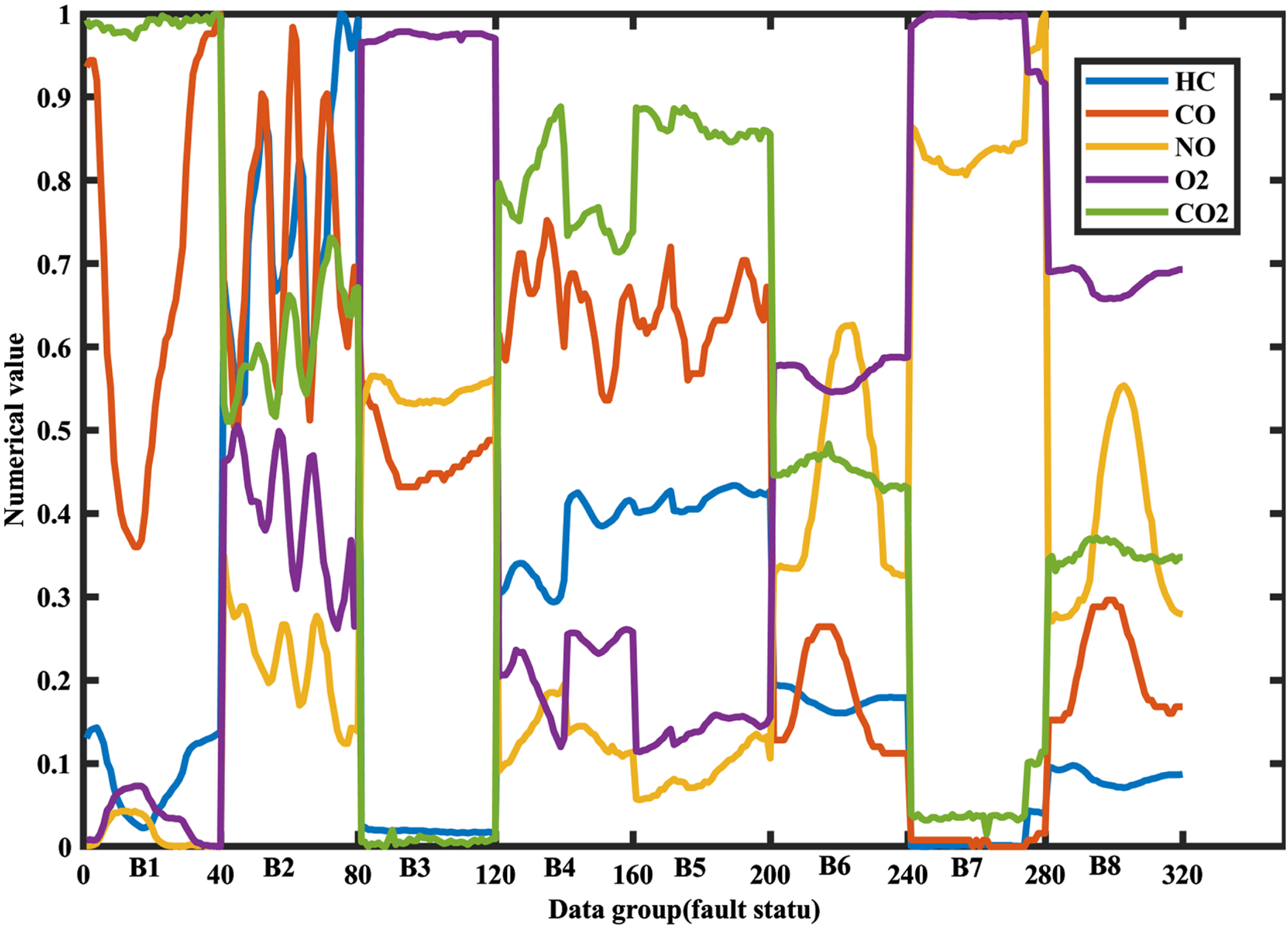
Data distribution map.

The above steps are repeated to collect engine exhaust data for 8 fault types. 8 fault types are normal (B1), ignition minor fault (B2), ignition severe fault (B3), throttle minor fault (B4), throttle severe fault (B5), injection minor fault (B6), injection severe fault (B7) and overlap fault (B8). Of these, minor faults are set to occasional (faults occurring at a frequency interval of 3 S or more) faults and severe faults are set to continuous faults. Overlapping faults are set to 2 different faults. The faults are all set on the control wire line. Forty sets of data were collected for each fault type and a total of 320 sets of experimental data were collected for the eight fault types.

Data normalisation. As the input sign vectors HC, CO, NO, O₂ and CO₂ have different ranges and units of values, the data need to be normalised to eliminate the effect of variable dimensionality on modelling accuracy. Equation (1) was used to normalise the volume fraction values of HC, CO, NO, O₂ and CO₂ to the interval [0, 1], respectively, according to the needs of this study. $y_{i} = \frac{X_{i} - X_{min}}{X_{max} - X_{min}}$ (1)

Where: x_min is the minimum value of the entire group of data, x_max is the maximum value of the entire group of data; x_i is the i-th input data; y_i is the normalized output value. The distribution of the data after normalisation is shown in Fig. 1.

3.2 Engine misfire fault diagnosis approach

3.2.1 Adaptive neural network fuzzy inference system

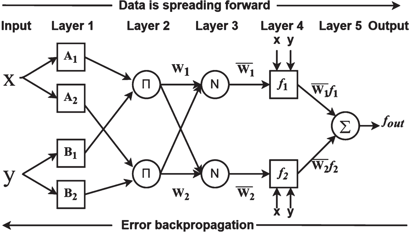
ANFIS [66] is a new fuzzy inference system based on the TS model proposed by J. S. R. Jang in 1993. ANFIS implements fuzzification, fuzzy inference, and anti-fuzzification using a neural network modeling approach, and can automatically generate If-Then rules. In order to reduce model complexity, this study is presented using a typical ANFIS system structural model, the structure of which is shown in Fig. 2 [67]. The system shown is a two-input, one-output five-layer structural network, which contains two if-then inference rules for the Takagi-Sugeno fuzzy model, with square nodes being system adaptive nodes, indicating that the parameters in these nodes are adjustable. Round nodes are fixed nodes, indicating that the parameters in these nodes are fixed and that each node in the same layer of the network has a similar function, and that the output data of the nodes in the previous layer will be the input data in the current layer.

Fig. 2

ANFIS structure diagram.

In Fig. 2, x and y are the two inputs of the system, and f_out is the output of the inference system, both of which are available data sets. The typical fuzzy inference rules R₁ and R₂ are: $R_{1} : If x is A_{1} and y is B_{1}, Then f_{1} = p_{1} x + q_{1} y + r_{1}$ (2) $R_{2} : If x is A_{2} and y is B_{2}, Then f_{2} = p_{2} x + q_{2} y + r_{2}$ (3)

The nodes of the first layer are adaptive nodes, represented by node functions, whose function is to blur the input signal and determine the degree to which a given input satisfies the corresponding fuzzy set. Use O_1,i to denote the output of the i-th node in the first layer, and so on. Node i has an output function: $O_{1, i} = μ A_{i} (x), i = 1, 2$ (4) $O_{1, i} = μ B_{i - 2} (y), i = 3, 4$ (5)

Among them, x and y are the inputs of node i, A_i and B_i are fuzzy sets, representing fuzzy meanings such as “Minor” and “Serious”; μA_i(x) and μB_i - 2(y) are membership functions, representing x, y It belongs to the degree of fuzzy set A_i, B_i (i = 1, 2). The membership function usually adopts a Gaussian function, the maximum value is equal to 1, and the minimum value is equal to 0, as shown below: $μ (x) = exp {\frac{- {(x - c)}^{2}}{2 σ^{2}}}$ (6)

Among them, {c,σ} are the premise parameters. It needs to be determined in advance. As the value of the premise parameter changes, the shape of the function will change. Therefore, the premise parameters should be set according to different mapping needs.

The nodes of the second layer are fixed nodes. The nodes of this layer are used to calculate the applicability of each rule, that is, multiplying the membership degrees of each input signal as the output signal. Its output signal W_i represents the activation intensity of the rule. $O_{2, i} = μ A_{i} (x) \cdot μ B_{i} (y) = w_{i}, i = 1, 2$ (7)

The nodes of the third layer are fixed nodes, and the node function is used to normalize the activation intensity by calculating the ratio of the activation intensity of the i-th node to the sum of the activation intensity of all rules. $O_{3, i} = \frac{w_{i}}{\sum w_{i}} = \frac{w_{i}}{w_{1} + w_{2}} = {\bar{w}}_{i}, i = 1, 2$ (8)

The nodes on the fourth layer are adaptive nodes, which are used to calculate the output of each rule. The node function is: $O_{4, i} = {\bar{w}}_{i} f_{i} = {\bar{w}}_{i} (r_{i} + p_{i} x + q_{i} y), i = 1, 2$ (9)

Among them, ${\bar{w}}_{i}$ is the normalized excitation intensity from the third layer, and {p_i, q_i, r_i} are the conclusion parameters.

The nodes on the fifth layer are fixed nodes, which play a role of defuzzification and get the total output of the system. $O_{5, i} = \sum_{i} {\bar{w}}_{i} f_{i} = \frac{\sum_{i} w_{i} f_{i}}{\sum_{_{i}} w_{i}} = f_{o u t}$ (10)

ANFIS contains the premise parameters {c, σ} and conclusion parameters {p_i, q_i, r_i} of the membership function. During the training process, these parameters can be continuously adjusted to achieve adaptive learning.

3.2.2 Subtractive clustering algorithm

In order to improve the recognition speed, recognition rate and stability of fault diagnosis. This study uses the Subtractive Clustering Method (SCM) to optimise the ANFIS to generate the initial Fuzzy Inference System (FIS) structure. This is because the SCM algorithm generates the initial FIS with a non-linear partitioning of the input space. This will reduce the complexity of the network model and thus increase the speed of operation. And while traditional ANFIS requires human settings to estimate the number of categories and cluster centres, the SCM algorithm is obtained automatically. This reduces the human influence and will improve the speed and stability of fault diagnosis.

The specific algorithm [67] is: Assuming a sample of M-dimensional n data points, X={x₁, x₂, . . . , x_n}, calculate the density value of each sample point x_i: $D_{i} = \sum_{j = 1}^{n} \exp (- \frac{{‖ x_{i} - x_{j} ‖}^{2}}{{(r \frac{a}{2})}^{2}})$ (11)

In the formula, r_a > 0 is the radius of the effective neighborhood of the cluster center. Select a sample point with the most surrounding data as the first cluster center. According to the cluster center, the density value of other data is calculated as: $D_{i} = D_{i} - D_{c}_{k} \sum_{j = 1}^{n} \exp (- \frac{{‖ x_{i} - x_{c}_{_{k}} ‖}^{2}}{{(r_{\frac{b}{2}})}^{2}})$ (12)

After screening and calculation, the kth cluster center and density values are x_ck and D_ck, respectively. r_b is the radius of the neighborhood where the density index is significantly reduced. In order to prevent the possible intersection of clustering, let r_b > r_a. Repeat the above calculation process, using formula (11) as the condition for the termination of the calculation. After the calculation, k is the number of cluster centers. $\frac{D_{c}_{_{k + 1}}}{D_{c_{1}}} < δ$ (13)

In the formula, δ<1, the larger the δ, the shorter the calculation time, and the fewer the cluster centers.

3.2.3 Parameter optimization of adaptive neural network fuzzy inference system

To improve the speed and quality of learning, the model parameters are decomposed into non-linear premise parameters and linear conclusion parameters, and a hybrid learning algorithm [68, 69] combining the BP (back propagation) algorithm and the LSE (least squares extimation) algorithm is used for parameter optimisation. Each stage of this hybrid learning process consists of forward and backward transfer.

The first is forward pass. First fix the premise parameters, and use the linear least squares estimation algorithm to optimize the conclusion parameters of the neural network. From Equations (2)–(10), the total output of the system can be expressed as a linear combination of conclusion parameters, namely: $f_{o u t} = \bar{w_{1}} f_{1} + \bar{w_{2}} f_{2} = \bar{w_{1}} (p_{1} x + q_{1} y + r_{1}) + \bar{w_{2}} (p_{2} x + q_{2} y + r_{2}) = (\bar{w_{1}} x) p_{1} + (\bar{w_{1}} y) q_{1} + \bar{w_{1}} r_{1} + (\bar{w_{2}} x) p_{2} + (\bar{w_{2}} y) q_{2} + \bar{w_{2}} r_{2}$ (14) Assumptions (15), (16), and (17): $f = {(f_{out 1}, f_{out 2}, \dots, f_{out 3})}^{T}$ (15) $θ = {(p_{1}, q_{1}, r_{1}, p_{2}, q_{2}, r_{2})}^{T}$ (16) $B = [\begin{matrix} \bar{w_{1}} x_{1} & \bar{w_{1}} y_{1} & \bar{w_{1}} & \bar{w_{2}} x_{1} & \bar{w_{2}} y_{1} & \bar{w_{2}} \\ \bar{w_{1}} x_{2} & \bar{w_{1}} y_{2} & \bar{w_{1}} & \bar{w_{2}} x_{2} & \bar{w_{2}} y_{2} & \bar{w_{2}} \\ ⋮ & ⋮ & ⋮ & ⋮ & ⋮ & ⋮ \\ \bar{w_{1}} x_{n} & \bar{w_{1}} y_{n} & \bar{w_{1}} & \bar{w_{2}} x_{n} & \bar{w_{2}} y_{n} & \bar{w_{2}} \end{matrix}]$ (17) Then Equation (14) can be expressed as Equation (18): $f = B \cdot θ$ (18) Suppose there are n items in the given training data. Define the overall error as: $E = \sum_{i = 1}^{n} E_{i} = \sum_{i = 1}^{n} {(T_{i} - f_{outi})}^{2}$ (19)

Where E_i is the ith error metric of the given training set, T_i is the expected output of the i-th input, and f_outi is the actual output of the i-th calculated by ANFIS.

According to the principle of least squares method, in order to minimize E, the least squares estimate θ* is: $θ * = {(B^{T} B)}^{- 1} B^{T} f$ (20)

In the forward pass, after each input vector is given, the corresponding node output is calculated until the matrices B and f in Equation (18) are determined, and the conclusion parameters are obtained by Equation (20).

The second step of parameter optimization is passed backward. Fix the conclusion parameters and calculate the error through Equation (19), and use the error back propagation method of gradient descent to make the error propagate from the output layer to the input layer. Use this to train and update the prerequisite parameters. Using the given sample data, repeat the above optimization steps until the error index requirement or the maximum number of training times is reached and the training process stops.

3.2.4 Fault diagnosis model performance evaluation

The performance of a fault diagnosis model is the key to achieving the fault diagnosis goal. In order to show the performance of the model more intuitively, three recognition rate indicators, one speed indicator and Excellent Rate (ER) were chosen to evaluate the performance of the model in this study. The three recognition rate metrics are root mean square error (RMSE), mean absolute percentage error (MAPE) and mean absolute error (MAE). The speed metric is the fault diagnosis model testing time (T). ER is the Excellent Rate of the SC-ANFIS model relative to other models in terms of recognition rate and speed, respectively. the equation for calculating the metrics is as follows. $RMSE = \sqrt{\frac{1}{n} \sum_{i = 1}^{n} {({\hat{y}}_{i} - y_{i})}^{2}}$ (21) $MAPE = \frac{100 %}{n} \sum_{i = 1}^{n} | \frac{{\hat{y}}_{i} - y_{i}}{y_{i}} |$ (22) $MAE = \frac{1}{n} \sum_{i = 1}^{n} | {\hat{y}}_{i} - y_{i} |$ (23) $T = t_{1} - t_{0}$ (24) $ER = \frac{A - B}{B} \times 100 %$ (25)

In the formula, $\hat{y}$ is the estimated value, and y_i is the actual value. n is the number of samples. t₀ is the start time, t₁ is the end time, A is the SC-ANFIS model indicator and B is other model indicators. The smaller the RMSE, the smaller the MAPE, the smaller the MAE and the smaller the T the better the model performance. A positive ER indicates that the SC-ANFIS model improves performance, and a negative ER indicates that the SC-ANFIS model reduces performance.

3.2.5 Simulation experiments of anfis network model based on subtractive clustering

The performance of an engine misfire fault diagnosis model directly determines the effectiveness of the fault diagnosis. Therefore, it is crucial to assess the performance of the engine misfire fault diagnosis model. Recognition rate, recognition speed and recognition stability are important performance indicators for fault diagnosis, so this study evaluates these three performances of the fault diagnosis model separately. The evaluation is based on the simulation results of the simulation platform software MATLAB.

Different input volumes and different sample sizes are 2 important factors in validating a network model. This is also true for the engine misfire fault diagnosis model. Therefore, this paper uses exhaust gas components with 3 different inputs (3, 4, 5) that have been proven to be useful for engine misfire fault diagnosis and 5 different sample sizes (10%, 30%, 50%, 70%, 90%) of the collected data to validate the network model.

In order to verify the superiority of SC-ANFIS in recognition rate, recognition speed and recognition stability of fault diagnosis. The traditional FCM-ANFIS [39] network model and the most used BP [70] network model were chosen for comparison. the parameters of the three network models are shown in Table 7. to enhance the validity of the comparison, each case was simulated and trained and tested 10 times respectively, and the results of the 10 simulations were used for comparison. the sample data for the 10 simulations were chosen randomly. The sample training data and test data used for the comparison models were the same for each case.

Table 7
Table of 3 network model parameters

Models SC-ANFIS FCM-ANFIS BP

Total number of floors 5 5 5

Learning Algorithm BP+LSE BP+LSE BP

maximum number of iterations 50 100 1000

Training error 0.0001 0.0001 0.00000001

Membership /activation Gaussian Gaussian Logsig

functions function function function

Number of membership Automatic 3n 0.001

functions/Learning Rate determination

Range of influence 0.5 Note: 3n denotes 3×n (n

Squash factor 0.7 denotes the number of

Accept ratio 0.2 dimensions of the input

Reject ratio 0.1 quantity)

Models	SC-ANFIS	FCM-ANFIS	BP
Total number of floors	5	5	5
Learning Algorithm	BP+LSE	BP+LSE	BP
maximum number of iterations	50	100	1000
Training error	0.0001	0.0001	0.00000001
Membership /activation	Gaussian	Gaussian	Logsig
functions	function	function	function
Number of membership	Automatic	3n	0.001
functions/Learning Rate	determination
Range of influence	0.5	Note: 3n denotes 3×n (n
Squash factor	0.7	denotes the number of
Accept ratio	0.2	dimensions of the input
Reject ratio	0.1	quantity)

The process for fault diagnosis based on the SC-ANFIS network model is shown in Fig. 3.

Simulation experiments with different inputs. 3 models were simulated 10 times with different inputs (3, 4 and 5). For the SC-ANFIS network model simulations with different inputs. Firstly, 90% (288 total data sets, 36 data sets for each of the 8 states) of the total sample data (320 total data sets, 40 data sets for each of the 8 states) of the 3 inputs (component values of HC, CO and NO) were randomly selected as training data, and the remaining 10% (32 total data sets, 4 data sets for each of the 8 states) of the data were used as test data. Next, the training data and test data were then fed into the network for simulation training and testing. The time and error values of the simulation tests are recorded. This is a 3-input simulation experiment. 10 simulations are conducted to improve the validity of the simulation experiment. 10 simulations are divided randomly. The simulation experiment is continued with 4 and 5 inputs according to the 3-input method. 4 inputs are the component values of HC, CO, NO and O₂; 5 inputs are the component values of HC, CO, NO, O₂ and CO₂. At the end of the SC-ANFIS network model simulation experiments with different inputs, the FCM-ANFIS and BP network models were carried out in the same way using the same simulation training, test data.

Fig. 3

Flow chart for SC-ANFIS based fault diagnosis.

Simulation experiments with different sample sizes. 3 models were simulated 10 times with different sample sizes (10%, 30%, 50%, 70%, 90%). The test data for the different sample size simulation experiments were all 10% of the total sample data. The sample data input volume was used with 4 inputs. The simulation experiments were conducted in the same way as the simulation experiments with different input amounts.

4 Results and discussion

The purpose of this simulation experiment is to validate the fault diagnosis performance of the proposed SC-ANFIS network model. The average of the simulation test results for the three network models with different input amounts and different sample sizes are shown in Tables 8 9.

Table 8
Average of the results of 10 simulations of the 3 models with different inputs

Inputs Models RMSE MAPE(%) MAE T

3 SC-ANFIS 0.1271 0.0174 0.0597 0.00661

FCM-ANFIS 0.1516 0.024 0.074 0.00668

BP 0.1311 0.0181 0.0687 0.00721

ER_{FCM - ANFIS}(%) 16.18 27.54 19.28 1.00

ER_BP(%) 3.06 4.09 13.08 8.32

4 SC-ANFIS 0.0113 0.002 0.0067 0.00652

FCM-ANFIS 0.0161 0.0024 0.0069 0.00676

BP 0.0123 0.0021 0.0072 0.00690

ER_{FCM - ANFIS}(%) 29.99 16.13 2.91 3.52

ER_BP(%) 8.03 2.41 7.12 5.47

5 SC-ANFIS 0.0114 0.0022 0.0071 0.00683

FCM-ANFIS 0.0131 0.0022 0.0059 0.00729

BP 0.0132 0.0023 0.0074 0.00734

ER_{FCM - ANFIS}(%) 13.09 1.41 -20.44 6.36

ER_BP(%) 13.47 2.81 4.05 7.00

Inputs	Models	RMSE	MAPE(%)	MAE	T
3	SC-ANFIS	0.1271	0.0174	0.0597	0.00661
	FCM-ANFIS	0.1516	0.024	0.074	0.00668
	BP	0.1311	0.0181	0.0687	0.00721
	ER_{FCM - ANFIS}(%)	16.18	27.54	19.28	1.00
	ER_BP(%)	3.06	4.09	13.08	8.32
4	SC-ANFIS	0.0113	0.002	0.0067	0.00652
	FCM-ANFIS	0.0161	0.0024	0.0069	0.00676
	BP	0.0123	0.0021	0.0072	0.00690
	ER_{FCM - ANFIS}(%)	29.99	16.13	2.91	3.52
	ER_BP(%)	8.03	2.41	7.12	5.47
5	SC-ANFIS	0.0114	0.0022	0.0071	0.00683
	FCM-ANFIS	0.0131	0.0022	0.0059	0.00729
	BP	0.0132	0.0023	0.0074	0.00734
	ER_{FCM - ANFIS}(%)	13.09	1.41	-20.44	6.36
	ER_BP(%)	13.47	2.81	4.05	7.00

Remarks: ER_{FCM - ANFIS} indicates the percentage of SC-ANFIS that is better than FCM-ANFIS. ER_BP indicates the percentage of SC-ANFIS that is better than BP.

Table 9

Average of 10 simulation test results for 3 models with different sample sizes

Sample	Models	RMSE	MAPE(%)	MAE	T
sizes
10%	SC-ANFIS	0.0508	0.0108	0.0284	0.00706
	FCM-ANFIS	0.1649	0.0266	0.0689	0.00820
	BP	0.2743	0.0675	0.1861	0.00830
	ER_{FCM - ANFIS}(%)	69.21	59.36	58.75	13.89
	ER_BP(%)	81.49	83.98	84.74	14.87
30%	SC-ANFIS	0.0283	0.0042	0.0141	0.00688
	FCM-ANFIS	0.0790	0.0122	0.0318	0.00748
	BP	0.0518	0.0108	0.0312	0.00715
	ER_{FCM - ANFIS}(%)	64.14	65.85	55.71	7.93
	ER_BP(%)	45.27	61.41	54.84	3.77
50%	SC-ANFIS	0.0174	0.0025	0.0092	0.00677
	FCM-ANFIS	0.0975	0.0138	0.0326	0.00731
	BP	0.0204	0.0030	0.0102	0.00720
	ER_{FCM - ANFIS}(%)	82.15	81.55	71.89	7.39
	ER_BP(%)	14.86	14.27	10.53	5.95
70%	SC-ANFIS	0.0131	0.0026	0.0079	0.00655
	FCM-ANFIS	0.0519	0.0079	0.0183	0.00684
	BP	0.0137	0.0029	0.0085	0.00696
	ER_{FCM - ANFIS}(%)	74.76	67.45	56.54	4.20
	ER_BP(%)	4.04	12.48	6.92	5.83
90%	SC-ANFIS	0.0113	0.002	0.0067	0.00652
	FCM-ANFIS	0.0161	0.0024	0.0069	0.00676
	BP	0.0123	0.0021	0.0072	0.00690
	ER_{FCM - ANFIS}(%)	29.99	16.13	2.91	3.52
	ER_BP(%)	8.03	2.41	7.12	5.47

Remarks: ER_{FCM - ANFIS} indicates the percentage of SC-ANFIS that is better than FCM-ANFIS. ER_BP indicates the percentage of SC-ANFIS that is better than BP.

4.1 Fault diagnosis recognition rate & stability

4.1.1 Various input quantities for rate & stability tests

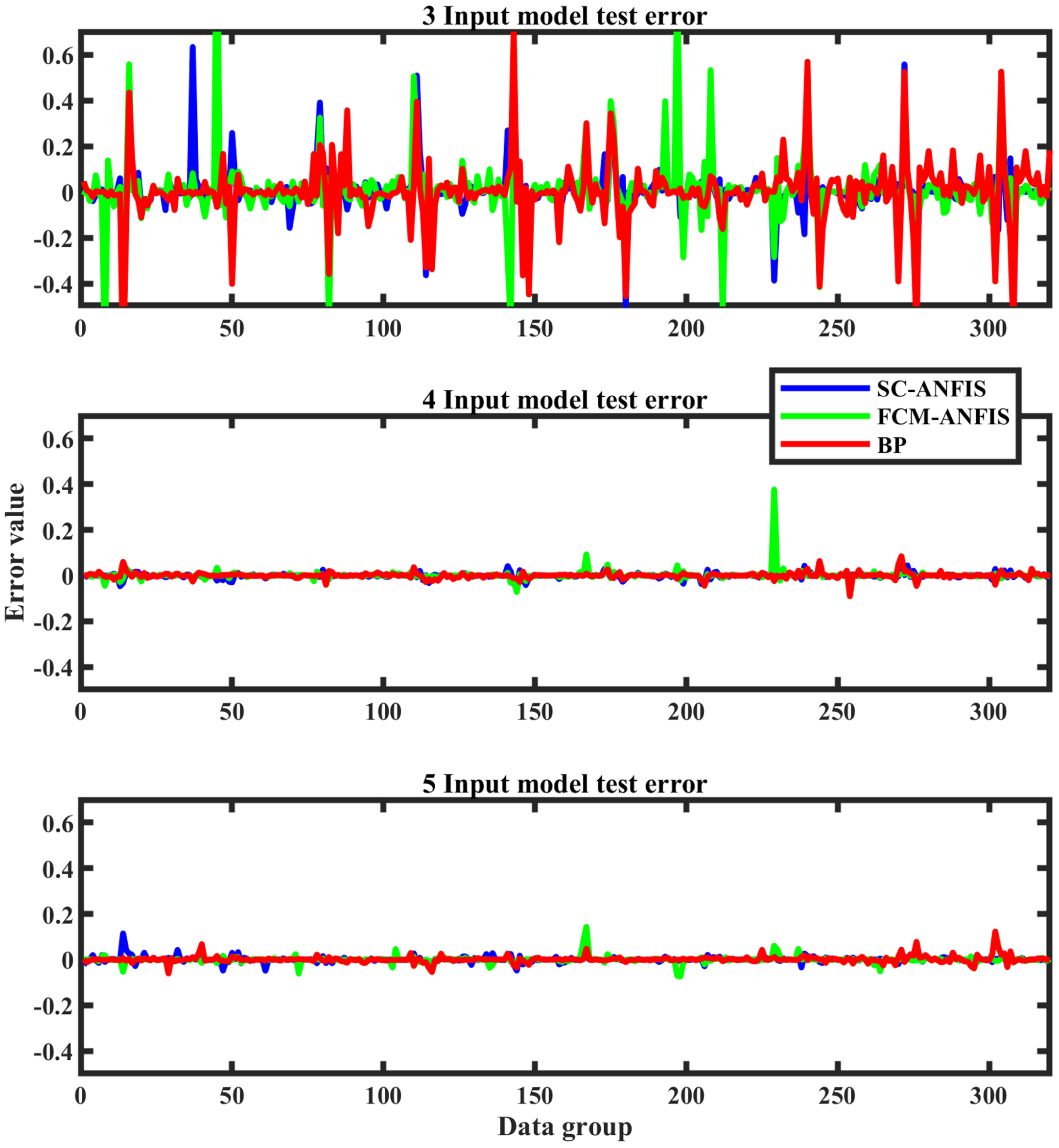
The mean values of the fault recognition rate metrics for the 3 models for 10 simulation tests with different input quantities are shown in Table 8. Comparative plots of the fault identification errors for the simulation tests of the 3 network models at different input quantities are shown in Fig. 4.

Fig. 4

Test errors for the 3 models with different inputs.

Fig. 5

Test errors for the 3 models at different sample sizes.

Observe Table 8. The SC-ANFIS model outperformed the FCM-ANFIS and BP models in terms of fault diagnosis recognition rate for different input quantities. 3 recognition rate indicators, RMSE, MAPE and MAE, had the smallest mean values for 10 tests. With 4 inputs, the SC-ANFIS model had the best fault diagnosis recognition rate, with its fault diagnosis recognition rate indicators RMSE (0.0113), MAPE (0.20%) and MAE (0.0067)) better than the FCM-ANFIS and BP models by 29.99%, 16.13%, 2.91%, 8.03%, 2.41%, 7.12%. In Fig. 4, the fault identification error and its stability of the blue line SC-ANFIS are better than those of the green line FCM-ANFIS and red line BP in the case of 3, 4 and 5 inputs. 320 sets of fault identification error data curves from 10 simulation tests with different inputs, the SC-ANFIS identification error curve has the least fluctuation, the most concentrated and smallest error values, and the most stable performance. Especially at 4 inputs, the performance is most obvious. At 3, 4 and 5, the magnitude of the fluctuation is: FCM-ANFIS>BP>SC-ANFIS.

Analysis: SC-ANFIS has better fault diagnosis recognition rate and stability than FCM-ANFIS for different input quantities. because (1) SC-ANFIS is non-linear partitioning for input space, FCM-ANFIS is using linear partitioning, while the engine exhaust component values are non-linear, SC-ANFIS based on non-linear mapping is better than FCM-ANFIS based on linear partitioning. (2) FCM-ANFIS is a random initial clustering centre, which affects the convergence performance of FCM-ANFIS and is easy to fall into local optimum, leading to the instability of clustering results. SC-ANFIS, on the other hand, is a density clustering algorithm that uses data points as a candidate set of clustering centres, which is more stable than the FCM-ANFIS algorithm. SC-ANFIS has a better recognition rate and stability than BP for different input quantities, because the initial weights and thresholds of the BP model are randomly assigned and optimised by the BP algorithm, which can easily fall into local optima, thus affecting the recognition rate. The parameters of the SC-ANFIS model are optimised using a hybrid learning algorithm combining the LSE algorithm and the BP algorithm, which can improve the disadvantage of the BP algorithm of easily falling into local optima.

4.1.2 Various sample sizes for rate & stability tests

The mean values of the fault identification rate metrics for the 3 models for 10 simulation tests with different sample sizes are shown in Table 9. Comparative plots of the fault identification errors for the simulation tests of the 3 network models at different sample sizes are shown in Fig. 5.

Observe Table 9 and Fig. 5. In Table 9, the SC-ANFIS model outperforms both the FCM-ANFIS and BP models in terms of fault diagnosis recognition rate for 5 different sample sizes. the mean of 10 tests for the 3 recognition rate metrics RMSE, MAPE and MAE are the smallest. Observe Fig. 5. for different sample sizes, the fault identification error and its stability of the blue line SC-ANFIS is better than that of the green line FCM-ANFIS and red line BP. the blue line SC-ANFIS is nearly covered by the green line FCM-ANFIS and red line BP. the fault identification error of the SC-ANFIS model curve has the least fluctuation, the error values are relatively the most concentrated and smallest, and the performance is the most stable. The performance is especially prominent at small sample sizes. The relationship between the magnitude of the fluctuations at different sample sizes is: FCM-ANFIS>BP>SC-ANFIS.

Analysis: SC-ANFIS has a better recognition rate and stability than FCM-ANFIS for different sample sizes because the cluster centre of SC-ANFIS is not related to the amount of sample data, but only to the density of sample data points. However, the clustering centre of FCM-ANFIS is related to the Euclidean distance of the sample data. At small sample sizes, the disadvantage that the FCM-ANFIS algorithm tends to fall into local optima is more likely to manifest itself. SC-ANFIS fault diagnosis recognition rate and stability is better than BP for different sample sizes. because the small sample size has less effect on the SC-ANFIS model than the BP model. Because of the fuzzy nature of engine misfire faults, the fuzzy clustering and fuzzy logic of SC-ANFIS play an advantage.

4.2 Fault diagnosis recognition speed & stability

4.2.1 Various input quantities for speed & stability tests

The mean values of the fault identification times for the 10 simulation tests for the 3 models with different input quantities are shown in Table 8. A comparison of the fault identification times for the 3 network models simulated and tested 10 times under different input quantities is plotted in Fig. 6.

Observing Table 8 and Fig. 6. In Table 8, the SC-ANFIS model outperformed both the FCM-ANFIS and BP models in terms of fault identification time for different input quantities. The SC-ANFIS model has the smallest mean value of 10 tests for fault identification time. The relationship between the mean recognition times is: BP (0.00721 s)>FCM-ANFIS (0.00668 s)>SC-ANFIS (0.00661 s) at 3 inputs; BP (0.00690 s)>FCM-ANFIS (0.00676 s)>SC-ANFIS (0.00652 s); at 5 inputs: BP (0.00734 s)>FCM-ANFIS (0.00729 s)>SC-ANFIS (0.00683 s). With the best fault diagnosis recognition rate of 4 inputs, the SC-ANFIS model has a better fault diagnosis recognition time than the FCM-ANFIS and BP models by 3.52% and 5.47% respectively. In Fig. 6, the fault identification time and stability of SC-ANFIS in blue line is better than FCM-ANFIS in green line and BP in red line for 3, 4 and 5 inputs. among the fault identification time data curves of 10 simulation tests with different inputs, the fault identification time curve of SC-ANFIS model has the least fluctuation and the most concentrated and smallest error value, the performance is the most stable. The relationship between the magnitude of the fluctuations is: FCM-ANFIS>BP>SC-ANFIS for 3 inputs, BP > FCM-ANFIS>SC-ANFIS for 4 inputs and BP > FCM-ANFIS>SC-ANFIS for 5 inputs.

Fig. 6

Test times for the 3 models with different inputs.

Analysis: The simulation test fault identification time and stability of the SC-ANFIS model is better than FCM-ANFIS for different input quantities because (1) SCM generates the initial FIS of ANFIS with a non-linear division of the input variables. This reduces the number of rules in the model, simplifies the model structure and reduces the amount of computation required to run the model, compared to the grid division of input variables in FCM-ANFIS. (2) SC-ANFIS model computation is determined by the number of samples independent of their dimensionality [71], while FCM-ANFIS model algorithm uses Euclidean distance, the dimensionality of the samples will affect the simulation time, especially the simulation training time, and will face the problem of dimensional disaster. The SC-ANFIS model is better than BP in terms of simulation test fault identification time and stability for different input quantities because (1) the computational effort of the SC-ANFIS model is independent of the number of sample dimensions, while the BP model becomes more complex and computational effort increases due to the increase in the number of sample dimensions. (2) The BP algorithm is a gradient descent algorithm, which has a strong local search capability but is prone to local minima and poor stability, whereas SC-ANFIS incorporates fuzzy logic and uses a hybrid learning algorithm based on neural networks, which has better stability.

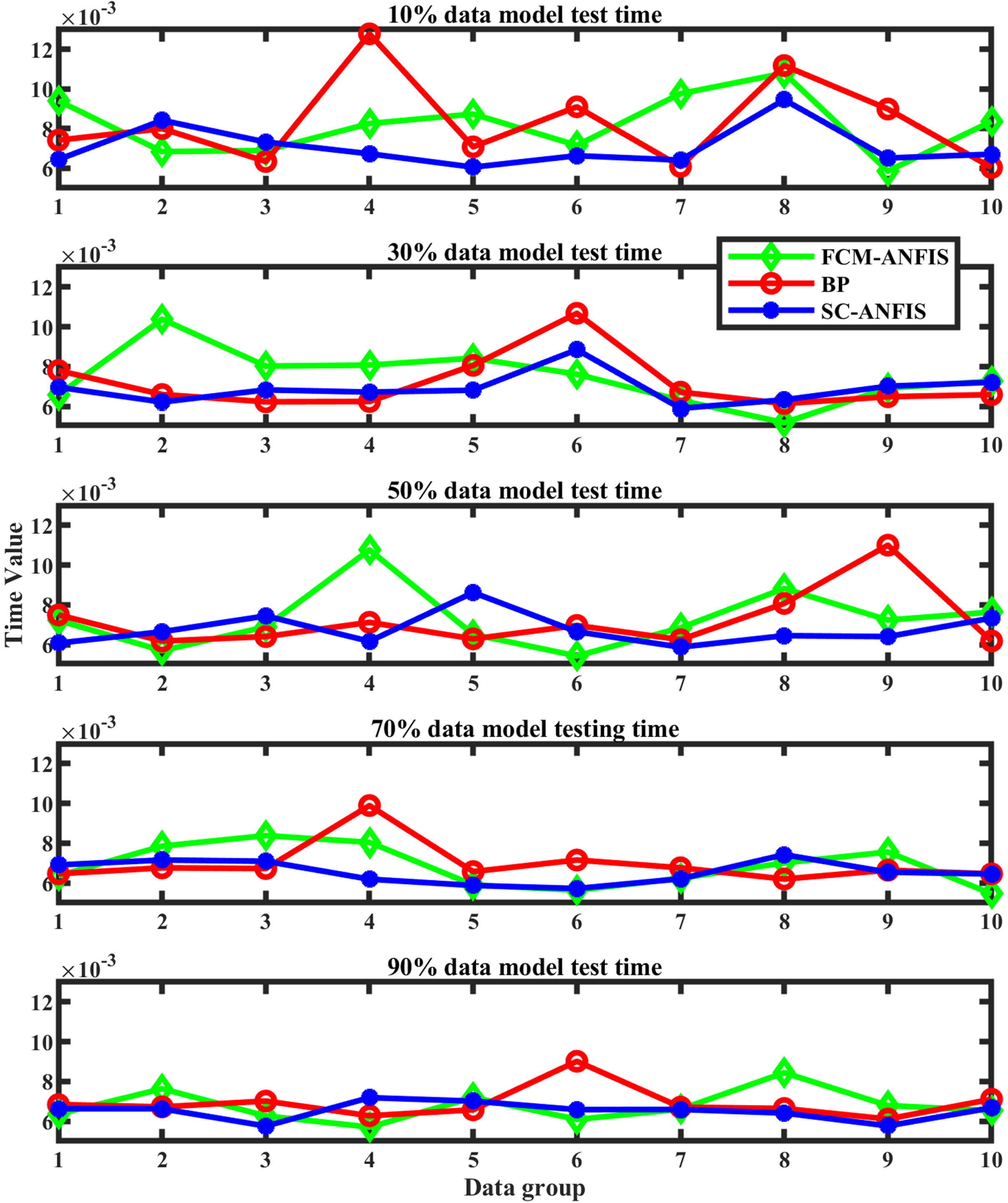
4.2.2 Various sample sizes for speed & stability tests

The mean values of the fault identification times for the 3 models for 10 simulation tests with different input volumes are shown in Table 9. A comparison of the fault identification times for the 3 network models simulated and tested 10 times with different sample sizes is plotted as shown in Fig. 7.

Observe Table 9 and Fig. 7. In Table 9, the SC-ANFIS model outperformed both the FCM-ANFIS and BP models in terms of fault identification time for different sample sizes. the SC-ANFIS model had the smallest mean value of 10 tests for fault identification time. The relationship between the magnitude of its average identification time as. At 10% sample size: BP (0.00830 s)>FCM-ANFIS (0.00820 s)>SC-ANFIS (0.00706 s); at 30% sample size: FCM-ANFIS (0.00748 s)>BP (0.00715 s)>SC-ANFIS (0.00688 s); at 50% sample size: FCM-ANFIS (0.00731s) >BP (0.00720s) >SC-ANFIS (0.00677s); at 70% sample size: BP (0.00696 s)>FCM-ANFIS (0.00684 s)>SC-ANFIS (0.00655 s); at 90% sample size: BP (0.00690 s)>FCM-ANFIS (0.00676 s)>SC-ANFIS (0.00652 s). Observe Fig. 7. The fault identification time and its relative stability of the blue line SC-ANFIS is better than that of the green line FCM-ANFIS and the red line BP for different sample sizes. in the fault identification time data curves of 10 simulation tests for different sample sizes, the SC-ANFIS model fault identification time curve has the smallest fluctuation amplitude, the most concentrated and smallest error value, and the most stable performance. The relationship between the magnitude of the fluctuations is as follows. BP > FCM-ANFIS>SC-ANFIS for 10%, 70% and 90% of the sample size; and FCM-ANFIS>BP>SC-ANFIS for 30% and 50% of the sample size.

Fig. 7

Test times for the 3 models at different sample sizes.

Analysis: The simulation test fault identification time and stability of SC-ANFIS model are better than FCM-ANFIS under different sample sizes. this is because (1) the model structure SC-ANFIS is simpler than FCM-ANFIS, so the SC-ANFIS model is less computationally intensive to run. (2) The selection of clustering centres is different. SC-ANFIS clustering centres are not affected by the amount of sample size, and the generated models are more stable than those generated by FCM-ANFIS, and its algorithm is also stable, resulting in a stable simulation test time. The simulation test fault identification time and stability of the SC-ANFIS model are better than the BP model for different sample sizes. This is because (1) the structure of the SC-ANFIS model is simpler than that of the BP model. (2) The parameter optimization algorithm of SC-ANFIS is a hybrid algorithm using a combination of BP algorithm and LSE algorithm, which reduces the number of dimensions of the search space in the BP algorithm and speeds up the testing speed. (3) The fuzzy mathematical algorithm is incorporated on the basis of neural network, which reduces the requirement of sample size data.

In summary. The SC-ANFIS model performs optimally for engine misfire fault diagnosis with different input amounts and different sample sizes. (1) The SC-ANFIS model has the best fault diagnosis recognition rate. The 3 indicators of fault diagnosis recognition rate, RMSE, MAPE and MAE, are smaller than those of the FCM-ANFIS and BP models in 2 different cases. The SC-ANFIS model has the best fault diagnosis recognition rate at 4 inputs. Its fault diagnosis recognition rate indicators RMSE (0.0113), MAPE (0.20%) and MAE (0.0067) were 29.99%, 16.13%, 2.91%, 8.03%, 2.41% and 7.12% better than the FCM-ANFIS and BP models respectively. (2) The SC-ANFIS model has the best fault diagnosis recognition speed. In 2 different cases, the SC-ANFIS model fault diagnosis recognition time is shorter than FCM-ANFIS and BP models. At the best fault diagnosis recognition rate of 4 inputs, the SC-ANFIS model had a better fault diagnosis recognition time (0.00652 s) than the FCM-ANFIS (0.00676 s) and BP (0.00690 s) models by 3.52% and 5.47% respectively. (3) The SC-ANFIS model has the best stability for fault diagnosis identification. In two different cases, (1) the stability of the fault diagnosis recognition rate of the SC-ANFIS model is better than that of the FCM-ANFIS and BP models; (2) the stability of the fault diagnosis recognition speed of the SC-ANFIS model is better than that of the FCM-ANFIS and BP models. Therefore, the SC-ANFIS model is the most suitable model for engine misfire fault diagnosis in this experiment.

5 Conclusion

In this study, a SC-ANFIS-based fault diagnosis model is proposed for engine misfire fault diagnosis. Under different input quantities (3, 4, 5) and different sample sizes (10%, 30%, 50%, 70%, 90%). The model improves the recognition rate, recognition time and recognition stability of fault diagnosis compared to the traditional FCM-ANFIS and BP network models. With the data and methods in this study, the fault diagnosis recognition rate metrics of the SC-ANFIS model amounted to RMSE (0.0113), MAPE (0.20%) and MAE (0.0067), which were better than the FCM-ANFIS and BP models by more than 2.91% and 2.41% respectively. The fault diagnosis recognition time of the SC-ANFIS model was 0.00652 s, which was 3.52% and 5.47% faster than the FCM-ANFIS (0.00676 s) and BP (0.00690 s) models, respectively. the stability of the fault diagnosis recognition rate and recognition time of the SC-ANFIS model was also better than that of the FCM-ANFIS and BP models.

The results of simulation experiments show that the engine misfire fault diagnosis model based on SC-ANFIS has the characteristics of high fault diagnosis recognition rate, fast recognition speed and good recognition stability, etc. SC-ANFIS is suitable for engine misfire fault diagnosis, which provides a theoretical basis and an idea for engine misfire fault diagnosis research and a method for solving practical problems. However, for the expected online real-time diagnosis, further research is needed to reach an efficient and convenient real-time diagnosis of engine misfire faults due to many reasons such as harsh engine working environment, real-time changes in operating status and untimely data collection.

Footnotes

Acknowledgments

The authors would like to acknowledge Faculty of Engineering, Universiti Malaysia Sabah for supporting this study.

References

Zheng

, Zhang

, Li

and Shi

, Real-time combustion torque estimation and dynamic misfire fault diagnosis in gasoline engine, Mechanical Systems and Signal Processing 126 (2019), 521–535. doi:10.1016/j.ymssp.2019.02.048.

Zhang

Y.B.

, Huang

, Wang

and Yan

, Power loss diagnosis method of internal combustion engine cylinder based on agent model, Machinery Design & Manufacture (08) (2020), 36–39+44. doi:10.19356/j.cnki.1001-3997.2020.08.009.

Norris

J.O.W.

, An In—service Emissions Test for Spark Ignition (SI) Petrol Engines—PPAD. United Kingdom, Oxford shire, EMStec Ltd, 2002, 09.

Wang

, Research and development of vehicle misfire generator for OBD system, Master Thesis, Wuhan University of Technology, Wuhan, 2006. doi:10.7666/d.y1020809.

, Research on gasoline engine exhaust emission prediction system based onOBDdata flow, Master Thesis, Nanjing Forestry University, Nanjing, 2019. doi:10.27242/d.cnki.gnjlu.2019.000272.

Liu

, He

, Xie

and Zhang

, Comparative study of Q3 injury in frontal impact test and offset test, Auto Time (04) (2021), 178–179+182. doi:10.3969/j.issn.1672-9668.2021.04.082.

Mao

C.Y.

and Ye

Z.C.

, Chief Editor, <<China Statistical Yearbook- 2019>> editorial board and editorial staff. China Statistical Yearbook. China Statistics Press, 4-5. doi:10.40049/y.cnki.yinfn.2019.000740.

Gosavi

M.A.

, Rhoades

B.B.

and Conrad

J.M.

, Application of Functional Safety in Autonomous Vehicles Using ISO 26262 Standard: A Survey, in SoutheastCon 2018, St. Petersburg, FL, Apr.2018, pp.1–6. doi:10.1109/SECON.2018.8479057.

Zhang

X.D.

, Misfire diagnosis of engine based on EEMD, Master Thesis, Jilin University, Jilin, 2017.

10.

Suda

J.L.

and Kagaris

, Automated diagnosis of engine misfire faults using combination classifiers, SAE International Journal of Commercial Vehicles 13(2) (2020), 103–114.

11.

Zhang

J.W.

, Research and Application of Fault Diagnosis Technology of Common Rail Diesel Engine, Master Thesis, Southeast University, Nanjing, 2018.

12.

Yang

, Evaluation of emission quality and fault diagnosis of internal combustion engine on plateau Research, PhD, Kunming University of Science and Technology, Kunming, 2019. doi:10.27200/d.cnki.gkmlu.2019.001901.

13.

Gao

W.Z.

, Wang

Y.J.

, Wang.

X.W.

, Zhang

, Li

and Dong

, Real-time diagnosis for misfire fault of diesel engine based on convolutional neural network, Journal of Jilin University (Engineering and Technology Edition) 52(02) (2022), 417–424. doi:10.13229/j.cnki.jdxbgxb20210777.

14.

, Li

, Yu

, Li

and Zeng

, Misfire fault diagnosis of automobile engine based on time domain vibration signal and probabilistic neural network, International Journal of Performability Engineering 16(9) (2020). doi:10.23940/IJPE.20.09.P18.14881496.

15.

Firmino

J.L.

, Neto

J.M.

, Oliveira

A.G.

, Silva

J.C.

, Mishina

K.V.

and Rodrigues

M.C.

, Misfire detection of an internal combustion engine based on vibration and acoustic analysis, J Braz. Soc. Mech. Sci. Eng. 43(7) (2021), 336. doi:10.1007/s40430-021-03052-y.

16.

Huang

Y.S.

and Zhang

, Misfire diagnosis base on fuzzy logic recognition, Journal of Chongqing University 35(S1) (2012), 37–40. doi:CNKI:SUN:FIVE.0.2012-S1-009.

17.

, Qiao

X.Y.

, Jin

and Han

L.J.

, Comparison of adaptive decomposition methods for multivariate signalof diesel engine, Vehicle Engine (06) (2020), 83–89. doi:10.3969/j.issn.1001-2222.2020.06.014.

18.

Zuo

H.S.

, Li

Z.Y.

, Lv

and Zhang

, Prediction of gasoline engine exhaust emission based on BP neural network, Journal of Jiangsu University (Natural Science Edition) 41(03) (2020), 307–313. doi:10.3969/j.issn.1671-7775.2020.03.010.

19.

S.W.

and Wang

J.H.

, Freeway car-following model and simulation based on adaptive neuro-fuzzy inference system, Journal of Tongji University (Natural Science) 38(07) (2010), 1018–1022. doi:10.3969/j.issn.0253-374x.2010.07.014.

20.

Long

H.H.

, et al., Integrated modeling of bed temperature for a circulating fluidized bed incinerator, Thermal Power Generation 46(02) (2017), 28–35. doi:10.3969/j.issn.1002-3364.2017.02.028.

21.

Lavanya

, Prasanth

, Jayachitra

and Shenbagarajan

, A Tuned classification approach for efficient heterogeneous fault diagnosis in IoT-enabled WSN applications, Measurement 8(3), 109771. https://doi.org/10.1016/j.measurement.2021.109771

22.

, Fault diagnosis for vehicle on-board equipments of high-speed railway based on GA-ANFIS model, Master Thesis, Lanzhou Jiaotong University. Lanzhou,2021, doi.org/10.27205/d.cnki.gltec.2021.001441.

23.

Chen

G.M.

and Miao

B.B.

, Ship course-keeping control design based on subtractive clustering adaptive neural-fuzzy inference, Ship Engineering (04) 82–87+139. doi:10.13788/j.cnki.cbgc.2019.04.15.

24.

Wang

Z.J.

and Wang

D.J.

, Engine misfire diagnosis based on probabilistic neural network, Journal of Jilin University (Information Science Edition) 34(02) (2016), 229–236. doi:10.19292/j.cnki.jdxxp.2016.02.011.

25.

J.-D.

and Liu

C.-H.

, An expert system for fault diagnosis in internal combustion engines using wavelet packet transform and neural network, Expert Systems with Applications 36(3) (2009), 4278–4286. doi:10.1016/j.eswa.2008.03.008.

26.

Zheng

T.X.

, Zhang

and Li

Y.F.

, Misfire fault diagnosis of automobile engine: A review, Acta Automatica Sinica 43(04) (2017), 509–527. doi:10.16383/j.aas.2017.c160276.

27.

Zhang

, Research on misfire fault diagnosis algorithm of automobile engine, Master Thesis, Chongqing University of Posts and Telecommunications, Chongqing, 2017. doi:CNKI:CDMD:2.1018.972367.

28.

Wang

, Wei

and Ye

, Misfire fault diagnosis of gasoline engines using the cosine measure of single-valued neutrosophic sets, Journal of New Theory 10 (2016), 39–44.

29.

and Dou

, Fault diagnosis of engine misfire based on genetic optimized support vector machine, in Proceedings of 2011 6th International Forum on Strategic Technology 1 (2011), 250–253. doi:10.1109/IFOST.2011.6021015.

30.

Liu

C.Y.

, Che

L.P.

and Bi

X.J.

, Engine fault identification based on TWSVM algorithm, Transactions of CSICE 37(01) (2019), 84–89. doi:10.16236/j.cnki.nrjxb.201901012.

31.

Karaboga

and Kaya

, Adaptive network based fuzzy inference system (ANFIS) training approaches: a comprehensive survey, Artif Intell Rev 52(4) (2019), 2263–2293. doi:10.1007/s10462-017-9610-2.

32.

Y.Z.

and Kang

D.L.

, Progress in Quantitative Structure-Activity Relationships Research of Antimicrobial Peptides, Food Science 36(15) (2015), 299–304. doi:10.7506/spkx1002-6630-201515055.

33.

Zhang

, Gao

W.Z.

, Gao

and Liu

, Misfire detection of diesel engine based on artificial neural networks, Journal of Vibration, Measurement & Diagnosis 40(04) (2020), 702–710+823. doi:10.16450/j.cnki.issn.1004-6801.2020.04.011.

34.

Wang

, Study on the Key Technology of Hoist Intelligent Fault Diagnosis in Network Environment, PhD, China University of Mining and Technology, Xuzhou, 2013. doi:CNK I:CDMD:1.1013.030094

35.

Chen

J.Y.

and Chen

Z.W.

, Present situation and development trend of failure diagnosis technology of the hydraulic system, Machine Tool & Hydraulics (10) (2008), 187–189+201. doi:10.3969/j.issn.1001-3881.2008.10.058.

36.

Gan

Y.T.

, Wu

Z.H.

, Chen

Z.C.

, Wu

L.J.

and Cheng

S.Y.

, Fault diagnosis system of photovoltaic array based on LoRa and adaptive network based fuzzy inference system, Electrical Engineering 21(08) (2020), 80–86. doi:10.3969/j.issn.1673-3800.2020.08.016.

37.

Fan

J.M.

, Wang

, Sun

Q.Q.

, Jiang

Q.J.

and Ou

M.H.

, Fault diagnosis and status evaluation for transformers using RVM and ANFIS, Proceedings of the CSU-EPSA 30(03) (2018), 35–41. doi:10.3969/j.issn.1003-8930.2018.03.005.

38.

S.L.

, “The Research of Assistant Diagnosis Model for Arrhythmia Based on ANIFS” [Master, Fudan University], Shanghai. 2009

39.

Yang

H.J.

, Research on Battery SOC Prediction Algorithm Based on Improved FCM and ANFIS, Master Thesis, Central ChinaNormal University, Wuhan, 2017. doi:CNKI:CDMD:2.1017.251408

40.

Zhu

S.M.

, Chen

C.F.

and Gao

, Creep model of red clay based on ANFIS neural network, Journal of Hunan University (Natural Sciences) (11) 137–145. doi:10.16339/j.cnki.hdxbzkb.2019.11.016.

41.

Shi

X.M.

and Hao

Z.Q.

, “<<MOHU KONGZHI JIQI MATLAB FANGZHEN (2nd Edition)>>”, Tsinghua University Press, Beijing Jiaotong University Press, 2018,03. ISBN: 978-7-5121-3455-3.

42.

Deng

Z.H.

, Zhang

D.D.

, Jiang

Y.Z.

, Liu

X.F.

and Wang

S.T.

, Multi-view fuzzy clustering algorithm based on partitionadaptive-fusion, Control and Decision 31(04) (2016), 593–600. https://doi.org/10.13195/j.kzyjc.2015.0057.

43.

Liu

S.W.

, Parallel diagnosing method on big monitoring data of electric power equipment based on storm framework, [Master, North China Electric Power University], Beijing, 2018.

44.

Yao

H.Y.

, Study on SOC estimation of ternary lithium battery based on genetic algorithms and improved BP neural network, [Master, Nanchang University], Nanchang. https://doi.org/10.27232/d.cnki.gnchu.2019.000962.

45.

Zhang

, Research on tillage resistance prediction of electric suspension based on adaptive fuzzy neural network, [Master, Nanjing Agricultural University], Nanjing. https://doi.org/10.27244/d.cnki.gnjnu.2019.001300.

46.

, Study on fault diagnosis method for diesel engine misfire based on vibration analysis in multiple signal fields and artificial neural network, Journal of Shandong Industrial Technology (02) (2021), 111–118. doi:10.16640/j.cnki.37-1222/t.2021.02.020.

47.

Rajput

and Parekh

, On-Board Diagnostics based remote emission test for Light MotorVehicles, in 2020 IEEE International Conference on Electronics, Computing and Communication Technologies (CONECCT), Jul. 2020, pp. 1–6. doi:10.1109/CONECCT50063.2020.9198374.

48.

Tan

Z.X.

, Liu

, Liang

J.X.

, Yang

X.D.

, Xie

T.P.

and Liang

B.Q.

, Judgment of diesel engine misfire cylinders based on crankshaft torsional vibration detection, Chinese Internal Combustion Engine Engineering 41(02) (2020), 70–76. doi:10.13949/j.cnki.nrjgc.2020.02.010.

49.

W.X.

, Tao

J.F.

, Qin

C.J.

and Liu

C.L.

, A diagnostic method for diesel engine misfire based on integrating of synchro-squeezed wavelet transform and xgboost, Journal of Xi’an Jiaotong University 53(02) (2019), 47–54+169. doi:10.7652/xjtuxb201902007.

50.

Ding

W.Q.

, Wang

J.Q.

, Hu

Z.J.

, Li

M.L.

, Dong

G.Y.

and Li

L.G.

, Discrimination of pre-ignition on gasoline engine based on lstm neural network and ionic current, Transactions of CSICE 40(02) (2022), 171–178. doi:10.16236/j.cnki.nrjxb.202202021.

51.

Cui

, et al., Optical diagnostics of misfire in partially premixed combustion under low load conditions, Fuel 329 (2022), 125432. doi:10.1016/j.fuel.2022.125432.

52.

Kassa

, Leroy

, Robert

and Vidal-Naquet

, Analysis of in-cylinder pressure oscillation and its effect on wall heat transfer, International Journal of Engine Research 22(7) (2189), 2189–2202. doi:10.1177/1468087420932364.

53.

Pagán Rubio

J.A.

, Vera-García

, Hernandez Grau

, Muñoz Cámara

and Albaladejo Hernandez

, Marine dieselengine failure simulator based on thermodynamic model, AppliedThermal Engineering 144 (2018), 982–995. doi:10.1016/j.applthermaleng.2018.08.096.

54.

Shahid

S.M.

, Ko

and Kwon

, Real-time abnormality detection and classification in diesel engine operations with convolutional neural network, Expert Systems with Applications 192 (2022), 116233. doi:10.1016/j.eswa.2021.116233.

55.

Wang

, Zhang

, Gao

, Li

, Wang

and Pang

, Misfire detection using crank speed and long short-term memory recurrent neural network, Energies 15(1) (2022), Art. no. 1. doi:10.3390/en15010300.

56.

Zhu

, Tan

M.K.

, Chin

R.K.Y.

, Chua

B.L.

, Hao

and Teo

K.T.K.

, Engine Fault Diagnosis using Probabilistic Neural Network, in 2021 IEEE International Conference on Artificial Intelligence in Engineering and Technology (IICAIET), Sep. 2021, pp. 1–6. doi:10.1109/IICAIET51634.2021.9573654.

57.

Zhang

, Gao

, Li

and Wang

, Misfire detection of diesel engine based on convolutional neural networks, Proceedings of the Institution of Mechanical Engineers, Part D: Journal of Automobile Engineering 235(8) (2021), 2148–2165. doi:10.1177/0954407020987077.

58.

Liu

J.M.

, Ma

and Jiang

Z.N.

, Probabilistic diagnosis of diesel engine misfire based on the noisy-max model and vibration signal from adjacent and opposite cylinders, Transactions of CSICE 38(06) (2020), 560–568. doi:10.16236/j.cnki.nrjxb.202006072.

59.

Q.F.

, Research on key technologies of fault diagnosis for high pressure common rail diesel engine, Master Thesis, Kunming University of Science and Technology, Kunming, 2020. doi:10.27200/d.cnki.gki.gkmlu.2020.000083.

60.

Xie

C.L.

, Zhang

J.Z.

and Wang

Y.C.

, Research on pattern recognition of engine misfire fault based on extension theory, Journal of Wuhan University of Technology (Transportation Science & Engineering) 42(03) (2018), 374–377. doi:10.3963/j.issn.2095-3844.2018.03.005.

61.

Zhang

J.Z.

, Research on engine misfire fault diagnosis based on vibration signal analysis, Master Thesis, Northeast Forestry University, Haerbin, 2017.

62.

Huang

W.Y.

, Wang

, Tian

X.L.

and Zhang

Y.H.

, Multi-mode engine fault diagnosis method based on SVR, Chinese Journal of Scientific Instrument 36(09) (2015), 2112–2119. doi:10.19650/j.cnki.cjsi.2015.09.025.

63.

X.J.

, Liu

C.Y.

and Lu

, Engine fault diagnosis method based on PSO-RVM algorithm, Journal of Harbin Engineering University 35(02) (2014), 245–249. doi:10.3969/j.issn.1006-7043.201303044.

64.

Che

L.P.

, Research on Fault Diagnosis of Automobile Engine Based on Machine Learning, Master Thesis, Harbin University of Science and Technology, Haerbin, 2019.

65.

Q.L.

, Research based on the optimization model of support vector machine for car-Engine misfire fault diagnosis, Master Thesis, Taiyuan University of Technology, Taiyuan, 2014. doi:10.7666/d.Y2692631.

66.

Jang

J.S.

, ANFIS: adaptive-network-based fuzzy inference system, IEEE Transactions on Systems, Man, and Cybernetics 23(3) (1993), 665–685. doi:10.1109/21.256541.

67.

Tang

, Xie

C.J.

, Zeng

M.M.

and Shi

, Fault diagnosis of power battery based on fuzzy neural network system, Chinese Journal of Power Sources 44(12) (2020), 1779–1783. doi:10.3969/j.issn.l002-087X.2020.12.018.

68.

Xie

, Niu

H.Y.

, Qi

D.Y.

and Ji

W.Z.

, Adaptive neural fuzzy inference system for prediction of traffic-related pollution, Fuzzy Systems and Mathematics 33(01) (2019), 143–153. doi:CNKI:SUN:MUTE.0.2019-01-016.

69.

Liu

Y.J.

, Zhang

T.X.

, Wen

B.C.

and Cao

W.K.

, Fault diagnosis of diesel engine based on anfis, Journal of System Simulation (21) (2008), 5836–5839. doi:10.16182/j.cnki.joss.2008.21.056.

70.

J.G.

, Chen

J.H.

and Ku

X.S.

, Review of gestures recognition based on vision, Computer Science 43(S1) (2016), 103–108. doi:CNKI:SUN:JSJA.0.2016-S1-027.

71.

Pei

J.H.

, Fan

J.L.

and Xie

W.X.

, A new initialization method of cluster centers, Journal of Electronics & Information Technology (03) (1999), 320–325. doi:CNKI:SUN:DZYX.0.1999-03-006.

Engine misfire fault diagnosis based on SC–ANFIS

Abstract

Keywords

1 Introduction

2 Literature review

2.1 Fault diagnosis using signal information

2.2 Fault diagnosis using diagnostic methods

3.1 Data collection for engine misfire fault

3.1.1 Selection for engine and signal information

3.2.1 Adaptive neural network fuzzy inference system

4.1.1 Various input quantities for rate & stability tests

4.2 Fault diagnosis recognition speed & stability

4.2.1 Various input quantities for speed & stability tests

Footnotes

Acknowledgments

References