Time and frequency domain pre-processing for epileptic seizure classification of epileptic EEG signals

Abstract

Although epilepsy is one of the most prevalent and ancient neurological disorder, but, still difficult to identify the specific type of seizure, due to artefacts, noise, and other disturbances, because of acquisition of Scalp EEG. It necessitating the use of skilled medical professionals as incorrect diagnosis lead to wrong Anti Seizure Drug (ASDs) and face it’s side effects. On the other hand machine learning plays a crucial role in seizure detection by analyzing and identifying patterns in brain activity data that are indicative of seizures. It can be used to develop predictive models that can detect the onset of seizures in real-time, allowing for early intervention and improved patient outcomes. Most of the research work focuses on seizure detection using various machine learning techniques pre-processed by different mathematical models. But, very less attention is paid towards seizure type detection. In this study, multiple Machine and Deep Learning algorithms were used in conjunction with time-domain and frequency-domain pre-processing to classify epileptic seizures into multiple types. The ictal period of various seizure types were extracted from Temple University Hospital EEG (TUHEEG) and the pre-processed data was tried out with multiple classifiers, including support vector classifiers (SVC), K- Nearest Neighbor (KNN), and Long short term memory (LSTM), among others. By using SVM, KNN, and LSTM, multiclass classification of seven types of epileptic seizures with 19 channels were considered for each EEG data and a 75–25 train–test ratio was accomplished with 90.41%, 94.46%, and 86.2% accuracy respectively. Epileptic seizure’s ictal phase EEG signals are categorized using a variety of machine learning(ML) and deep learning(DL) methods after being pre-processed using time domain and frequency domain approaches. The KNN yields the best results of all.

Keywords

Seizure classification TUHEEG ABSZ CPSZ FNSZ GNSZ SPSZ TNSZ TCSZ SVM KNN LSTM EEG

1 Introduction

Worldwide, the categorization of epileptic seizures is a relatively popular research area. Although epilepsy is one of the most common and ancient neurological conditions, there hasn’t been a substantial advancement in its diagnostic or therapeutic features despite decades of research on a global scale. Out of various reasons, the predominant reasons are:

The interconnectedness of epilepsy and brain waves. This throws an extreme challenge to clinicians towards seizure identification in the presence of artefacts and noise. The removal of artefact and noise is the prime goal of many researchers [1, 2].

The EEG signals are non-stationary, and their statistical characteristics vary over time and across patients.

Though EEG is a random signal, still due to its accessibility, cheap cost, and non-invasive nature, it is a great tool for examining cerebral activity in both clinical and research settings. The EEG is the gold standard test in the clinic for identifying and diagnosing epilepsy, stroke, and a wide range of other trauma- and pathology-related diseases [3, 4]. EEG is utilized in research labs to examine brain-computer connections, motor planning and execution, and neural reactions to external stimuli [5]. While there is currently no substitute for human interpretation when it comes to EEG analysis in the clinic, a variety of software tools are available to speed up the procedure or do analyses that are predictive [6], such as seizure prediction, but yet to be implemented in real-time. On the other side, miss interpretation leads to a heuristic approach of prescribing Anti Seizure Drugs(ASDs) having adverse side effects. Therefore, it’s crucial to correctly identify the seizure type [7 –9].

c) The quality of the data sets employed for the ML and DL task.

To improve the precision of type detection using EEG signals, firstly, the most important role is played by a large dataset having varieties of seizure type data and it’s relevant information. And secondly, it requires appropriate methods to extract features and analyse the same with greater accuracy. Ironically, given that hundreds of thousands of EEGs are performed every year in clinical settings all over the world, there are very few data that are publicly available. In a form that is helpful for ML research, only a small portion of this data is publicly accessible to the research community. Modern ML [10, 11] and DL algorithms [12, 13] could be used to find novel diagnoses and confirm clinical practice using vast amounts of EEG data. Furthermore, as “clinical-grade” data is intrinsically more variable with respect to factors like electrode position, clinical environment, equipment, and noise, it is preferable that such data be obtained in clinical settings as opposed to strictly controlled research environments. The creation of reliable, high-performing technology with practical application depends on capturing this fluctuation. The dataset created by TUHEEG fulfils the requirement of a good dataset. In this, textual physician reports that describe the patients and scans have been combined with the records, which have been edited, sorted, and curated. The Neural Engineering Data Consortium makes the corpus available to the general audience. It is the largest open-source corpus of its kind, and accurately characterizes clinical conditions [14]. The TUSZ data collection is intricate and offers a wide range of patients, seizures, and EEG montages (the placement of the electrodes). Deep architectures are the foundation of the ML models that have been proposed [15, 16], however, the results are not yet compelling. TUSZ already provided more patients and a larger range of seizure types for the studies than the other seizure corpora, and the most recent versions provided even more. In this work, seven seizure-type EEG signals are extracted from TUSZ.

A good dataset followed by appropriate algorithms builds a complete system. In literature, numerous mathematical models, algorithms, and techniques have been used. Machine and Deep Learning introduction has boosted classification accuracy and raised the possibility of real-time diagnosis support.

The results presented were the first ones on this data set to be reported, and several structures are extensively described [17]. In this study, the authors provide a total of 50 patients for testing and a total of 64 patients on whom algorithms were trained. Hidden Markov Models (HMM), Long Short-Term Memory (LSTM), Convolutional Neural Networks (CNN) coupled with MultiLayer Perceptrons (MLP), and a hybrid CNN/LSTM model are among the designs used. Principal component analysis, or (Incremental) PCA, is typically used to reduce dimensionality. The hybrid CNN/LSTM model, however, achieves an exceptional specificity of 96.86%, resulting in a very low false alarm rate of 7 FA/24 hours.

A related study employs Gated Recurrent Units (GRU), a type of Recurrent Neural Network (RNN) that is faster than LSTM but less accurate [18, 19]. Using EEG data from the Temple University Hospital (TUH) database [17], classified the various types of epileptic seizures [20] as follows: Simple Partial Seizure (SPSZ), Complex Partial Seizure (CPSZ), Focal Non-Specific Seizure (FNSZ), Absence Seizure (ABSZ), Generalized Non-Specific Seizure (GNSZ), Tonic-clonic Seizure The 0,1-44 Hz band pass filter was applied to the 19 channel EEG data. In order to determine the most appropriate network, Alexnet, Vgg16, Vgg19, Squeezenet, Googlenet, Inceptionv3, Densenet201, Resnet18, Resnet50, and Resnet101 networks were evaluated. The highest classification accuracy was achieved as 82.85% (Googlenet) and 88.30% (Resnet18, Resnet50, and Resnet101), respectively (Inceptionv3). It has been demonstrated that the Convolutional Neural Network (CNN)-based methodology [21] performs better than conventional methods. In [22], identified three types of EEG activity using EEG data from the Karunya Institute of Technology and Science (KITS) and TUH database: normal, generalised, and focused. The remaining 40% of the data was utilised for testing, and 60% for training. Utilizing the Tunable-Q Wavelet Transform, the data was banded (TQWT). For each sub-band, the entropies of log energy, Shannon, and Stein Unbiased Risk Estimation (SURE) were determined. Particle Swarm Optimization (PSO) was used to do the feature reduction, while Artificial Neural Networks (ANN) were chosen as the classifier of choice. Four classifications (normal-focal, normal-generalized, normal-focal + generalised, and normal-focal-generalized) with a maximum classification accuracy of 100% were obtained in the study using the KITS database. In the study using the TUH database, four different categorization models with 15 characteristics each had a success rate of 95.1%, 97.4%, 96.2%, and 88.8%. Roy et al. divided the eight kinds of epileptic seizures into myoclonic seizures (MYSZ), FNSZ, GNSZ, SPSZ, CPSZ, ABSZ, TNSZ, and TCSZ. [23]. The KNN, Stochastic Gradient Descent (SGD), Xgboost, and CNN stochastic classifiers were used to classify the data, and the results were compared. A weighted F1 score of 0,901 for v1.4.0 data with five-fold cross validation and a weighted F1 score of 0,561 for v1.4.0 data were obtained using the KNN classification algorithm. EEG data from the scalp was produced utilising 5.2 data with three-fold cross validation using the Xgboost classification method, and it was found to be a criterion for categorising multiclass seizure types. In [24], classified the signals from the epileptic region and the signals from the non-epileptic region (focal, non-focal) using two separate EEG databases (Berne-Barcelona dataset and seizure identification datasets). Data was divided into two-second epochs and filtered with a band pass of 0.5 to 150 Hz. The features are created using wavelet, Fourier decomposition, and empirical mode transformations. A classification success rate of over 95% was achieved in this work using five-fold cross-validation with the Bern-Barcelona EEG dataset and around 70% with the seizure identification datasets.

Deep neural networks are structures with more hidden layers than normal neural networks or so-called shallow networks [13, 23]. The number of network parameters increases dramatically as networks get bigger, necessitating adequate learning strategies as well as precautions against overfitting the taught network. Convolutional networks drastically reduce the number of trainable parameters by using filters convolved with input patterns rather than multiplying a weight vector (matrix).

Apart from the above-mentioned methods, in literature varieties of mathematical models are used as pre-processing techniques along with signal-analyzing methods. Segment-wise seizure categorization using a multiresolution directed transfer function method on epileptic EEG signals [25], using extreme gradient boosting classifier [26], based on domain-invariant deep representation of EEG [27], deep feature extraction based method [28], variable weight algorithm for CNN [29], multi-spectral deep feature learning [30, 31], using recurrence plots [32], using deep batch normalization neural network [33], using Neural Memory Networks [34], etc. are few of the techniques among many.

Though seizure classification is the most popular research interest, and a good amount of research work is available in the Ictal stage, but not in Pre-Ictal and Inter-Ictal stages. And also very less focus on the detection of seizure types in other stages apart from Ictal stage.

In this work the classification of seven types of seizure in three stages are carried out. The paper is structured as follows: Section 2 provides details on the methodology to be used and the procedures to be followed. The article’s analysis findings are presented in Section 3. Topics pertaining to the findings and possible future research projects are covered in Section 4.

2 Methodology

The methodology followed in this paper is depicted in Fig. 1. In this work, to start with EEG signals are extracted for seven types of seizures. In step 2, the labelled signals are treated in three ways; a) time domain pre-processed, b) frequency domain pre-processed [35], and c) raw data (without any pre-processing). In step 3 the machine and deep learning models are trained using a 75-25 train-test ratio. In step 4, using the trained model the seizure-type prediction is accomplished.

Fig. 1

Methology adopted for seizure type detection.

2.1 Data extraction

The extensive collection of clinical EEG data from the Temple University EEG Corpus (TUH EEG Corpus) [22] spans more than ten years. The data, which is 24 to 36 channels of signal data sampled at 250 Hz with 16 bits per sample, is stored in EDF (European Data Format) files. The annotations follow the TCP channel configuration, whereas the selected data adheres to the average reference configuration (AR). Each EDF file is accompanied by a neurologist’s anonymous report, which includes the patient’s medical history, such as seizure symptoms and prescription information, as well as the patient’s age, gender, and seizure frequency. It also provides analysis and observations from the clinician regarding seizure events. The versions of the files used were v1.5.0, which was released in March 2019, and v1.4.0. The corpus includes 10 different forms of seizures: focal non-specific (FNSZ), generalised non-specific (GNSZ), simple partial (SPSZ), complex partial (CPSZ), tonic (TNSZ), tonic-clonic (TCSZ), absence (ABSZ), clonic (CNSZ), atonic (ATSZ), and myoclonic (MYSZ). The first seven types are used to assess a multiclass classification with the number of events 57, 54, 55, 54, 53, 52, 47 respectively. The total number of seizures that could be estimated from the data obtained is 30667.7655 seconds. Additionally, the corpus includes funda-mental patient data including age, gender, prescription information, and medical history. The patients were between the ages of 27 and 91. The exact signal at the moment the seizure occurred has been recovered from the EDF file that has been extracted from the dataset using the seizure start time and stop time provided in the excel file. As demonstrated in Table 1, the primary four classifications of seizures are taken into account in this work.

Table 1
Seizure types and descriptions

Seizure code Name Description Samples NE

^aABSZ Absence Seizure Absence discharges are seen on the EEG. Loss of awareness is a symptom. 96668 57

^aCPSZ Complex Partial Seizure Day dreaming and blank stares are signs of loss of awareness of one’s surroundings. 922447 54

^bFNSZ Focal Seizure Starts in one part of the brain, but can spread to other parts i.e. become generalized. 324887 55

^bGNSZ GeneNon-Specific Seizure Seizures that are generalized and cannot be further characterized. Symptoms include stiffness, spasms, and unconsciousness. 447487 54

^aSPSZ Simple Partial Seizure There is no change in awareness. Body muscles are impacted. 541605 53

^aTNSZ Tonic Seizure Tensing of the muscles 1089507 52

^aTCSZ Tonic-Clonic Seizure Stiffness at first, then jerking of the body (Grand Mal) 240479 47

Seizure code	Name	Description	Samples	NE
^aABSZ	Absence Seizure	Absence discharges are seen on the EEG. Loss of awareness is a symptom.	96668	57
^aCPSZ	Complex Partial Seizure	Day dreaming and blank stares are signs of loss of awareness of one’s surroundings.	922447	54
^bFNSZ	Focal Seizure	Starts in one part of the brain, but can spread to other parts i.e. become generalized.	324887	55
^bGNSZ	GeneNon-Specific Seizure	Seizures that are generalized and cannot be further characterized. Symptoms include stiffness, spasms, and unconsciousness.	447487	54
^aSPSZ	Simple Partial Seizure	There is no change in awareness. Body muscles are impacted.	541605	53
^aTNSZ	Tonic Seizure	Tensing of the muscles	1089507	52
^aTCSZ	Tonic-Clonic Seizure	Stiffness at first, then jerking of the body (Grand Mal)	240479	47

2.2 Pre-processing

Each signal has been divided into seizure event zones using the start and stop length of seizures provided by the corpus, and the same has been converted to CSV format. These CSV data were pre-processed before being entered into any model because each row in each file represented a channel. The data had a variable number of channels across all the files, and as the last few channels in the signals typically belong to background signals, a common value of 19 channels was chosen. The files were then assigned the labels 0, 1, 2, 3,4,5 and 6, respectively, for ABSZ, SPSZ, FNSZ, GNSZ, TCSZ, TNSZ, and CPSZ. Also eliminated were about 79 columns that were discovered to be empty. It was discovered that the samples’ lengths weren’t equal. In this work, three approaches are adopted a) time domain pre- processing approach, b) frequency domain pre-processing approach c) raw data without pre- processing approach.

2.2.1 Time Domain pre-processing

The type of seizure depends on the pattern of occurrence in the channels, not on the number of seizure occurrences in the same channel. The signals were repeated till a length of 16384 samples in order to balance the lengths without losing frequency information. The matrix of seizure kinds was expanded to 10166×16384 by adding a label column. The last column of the matrix, measuring 10166×16385, included the labels.

2.2.2 Frequency domain pre-processing

In this approach, each labeled EEG signal are passed through inner multiplication, as for eg, if one subject has an EEG pattern S1 = C×IL, where C represents the number of channels and IL represents the length of the sequence during the ictal period. The feature of the S1 is stored as f(m,n) = S1×S1*, where S1* represents the transpose of S1 and stored as a square matrix of 19×19 as 19 channels are extracted. This 2D feature matrix is transformed to the frequency domain using discrete Fourier transform (DFT), discrete cosine transform (DCT) [36], and Hilbert transform (HT), and the energy of each pattern is stored based on labels.

2.2.2.1. DFT. The two-dimensional (2D) forwards and inverse fast Fourier transform [37] is shown in equation (1) and equation (2) respectively where N = 19 and F(u,v) is the frequency domain counterpart of f(m,n), a square matrix of size 19×19.

$\begin{matrix} F (u, v) \\ = \frac{1}{\sqrt{N}} \sum_{m = 0}^{N - 1} \sum_{n = 0}^{N - 1} f (m, n) e^{- j 2 π (u \frac{m}{N} + v \frac{m}{N})} \end{matrix}$ (1)

$\begin{matrix} f (m, n) \\ = \frac{1}{\sqrt{N}} \sum_{u = 0}^{N - 1} \sum_{v = 0}^{N - 1} F (u, v) e^{- j 2 π (u \frac{m}{N} + v \frac{n}{N})} \end{matrix}$ (2)

The same forward and inverse fast fourier transform can be obtained using the matrix method as shown in Equations 4), where W represents the twiddle factor matrix.

${[F]}_{N \times N} = [W^{*}]_{N \times N} [f]_{N \times N} [W^{* T}]_{N \times N}$ (3)

$[f]_{N \times N} = [W^{* T}]_{N \times N} [F]_{N \times N} [W^{*}]_{N \times N}$ (4)

The [F] obtained by Equation (3) is sparse and the prominent coefficients are stored in feature space.

2.2.2.2. DCT. The two-dimensional (2D) forwards DCT is shown in Equations 6) whereas, inverse DCT is shown in Equation (7).

$\begin{matrix} F (u, v) = & \frac{1}{N} \sum_{m = 0}^{N - 1} \sum_{n = 0}^{M - 1} f (m, n); \\ if u = 0 and v = 0 \end{matrix}$ (5)

$\begin{matrix} F (u, v) = \frac{2}{N} \sum_{m = 0}^{N - 1} \sum_{n = 0}^{M - 1} f (m, n) cos \\ [\frac{(2 m + 1) u π}{2 N}] cos [\frac{(2 n + 1) v π}{2 N}] \\ If u \neq 0 and v \neq 0 \end{matrix}$ (6)

$\begin{matrix} f (m, n) = & \frac{2}{N} \sum_{u = 0}^{N - 1} \sum_{v = 0}^{M - 1} F (u, v) cos \\ [\frac{(2 m + 1) u π}{2 N}] cos [\frac{(2 n + 1) v π}{2 N}] . \end{matrix}$ (7)

Matrix form of forward and inverse DCT is shown in Equations 9) respectively. Where C is the coefficient of DCT, a real-valued matrix.

$[F]_{N \times N} = [C]_{N \times N} [f]_{N \times N} [C^{T}]_{N \times N}$ (8)

$[f]_{N \times N} = [C^{T}]_{N \times N} [F]_{N \times N} [C]_{N \times N}$ (9)

The [F] obtained by Equation (8) is sparse real valued matrix and the distinct coefficients are stored in feature space.

2.2.2.3. HT. F(w) in the discrete time Fourier transform (DTFT) is [-isgn(w)F(w)] in the case of the Hilbert transform (HT), according to [38, 39]. Since F(w) does not contain an impulse at the origin and |-isgn(w)| = 1 except for w = 0,

$\frac{1}{2 π} \int_{- \infty}^{\infty} {| - isgn (w) F (w) |}^{2} dw = \frac{1}{2 π} \int_{- \infty}^{\infty} | F (w) |^{2} dw .$ (10)

$H [K] = - isgn (\frac{N}{2} - k) sgn (k)$ (11)

$h [n] = \frac{2}{N} \sum_{k = 1}^{\frac{N - 1}{2}} H [K] sin (\frac{2 π kn}{N})$ (12)

Equation (10) reveals that the energy characteristics of the DTFT and Hilbert transform are identical. Discrete Hilbert transform equation is shown in Equations 12).

2.2.3 Raw data

The EEG signals in this case is unprocessed [40]. As in TUSZ corpus EEG signals available from 26 channels to 34 channels from that 19 channels which are connected to Fp1, Fp2, F7, F3, Fz, F4, F8, T3, C3, Cz, C4, T4, T5, P3, Pz, P4, T6, O1, O2 points of 10–20 international systems are extracted.

2.3 Training machine and deep learning models

Each of these 3 sets of the labeled dataset is split into 75-25 train-test ratios and different ML and DL algorithms with and without hyperparameter tuning are carried out for 1st two sets but the last set ie raw data used only for the LSTM model because of unequal sequence length.The ML and DL models used in this study are as follows:

2.3.1 Support Vector Classifier (SVC)

For both classification and regression issues, the Support Vector Machine (SVM) method, is one of the most popular supervised learning technique. It is known as Support Vector Classifier when it is used to solve Machine Learning Classification issues (SVC) and widely used for both binary and multiclass classifications. On other side Support Vector Regression (SVR) solves regression issues.

Multiclass classifications performed using threeways: i) OVO (One Vs One) and ii) OVA (One Vs All) iii) AVA (All Vs All). Figure 2 shows AVA of seven class SVC.

Fig. 2

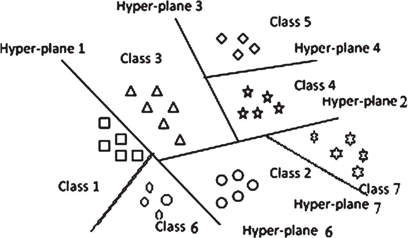
Linear multiclass SVM.

The following data is classified using the relevant hyperplanes by a linear SVC. Equation (13) contains the hyperplane equation for a two-dimensional plane:

$H : ω^{T} (x) + b = 0$ (13)

Where b is the intercept/bias and w(x) is the weight matrix.

The Lagrange technique is used to determine the ideal values of w and b, as shown in Equation (14). The lamda is used for optimization of weight. The differentiation of error (E) with respect to w and equate to zero i.e. $\frac{\partial E}{\partial w} = 0$ , from this condition λ is determined. Once the value of lambda(λ) has been determined, the formula

$w = \sum_{i = 1}^{l} λ_{i} y_{i} x_{i}$ (14)

is used to determine the ideal value of weights (w).

2.3.2 K Nearest Neighbour (KNN)

The K-Nearest Neighbors (KNN) technique is based on the idea that data points with similar characteristics are more likely to be located close together in a plane. The ‘K’ nearest neighbours are used in this classification process to group data points into different categories. The data will be given the class of its nearest neighbour, for instance, if the value of K is assumed to be 1 and the blue hexagon serves as the test sample then it classifies as red class, as in Fig. 3. If K = 3 and K = 9 nearest neighbours are represented by two condensed circles. Since there are two red balls close to the test sample in this example for K = 3 and only one green ball, the test sample is categorised as belonging to the red class in this instance. On the other hand, for K = 9, there are three green balls as opposed to two red balls and one black, orange, light blue, violet ball. The test sample will be categorised as green class for K = 9. Due to this uncertainty, researchers prefer to choose K = 1, which typically yields better results than other values of K. Based on Euclidean distance, as shown in Equation (16), the closest neighbours are identified.

Fig. 3

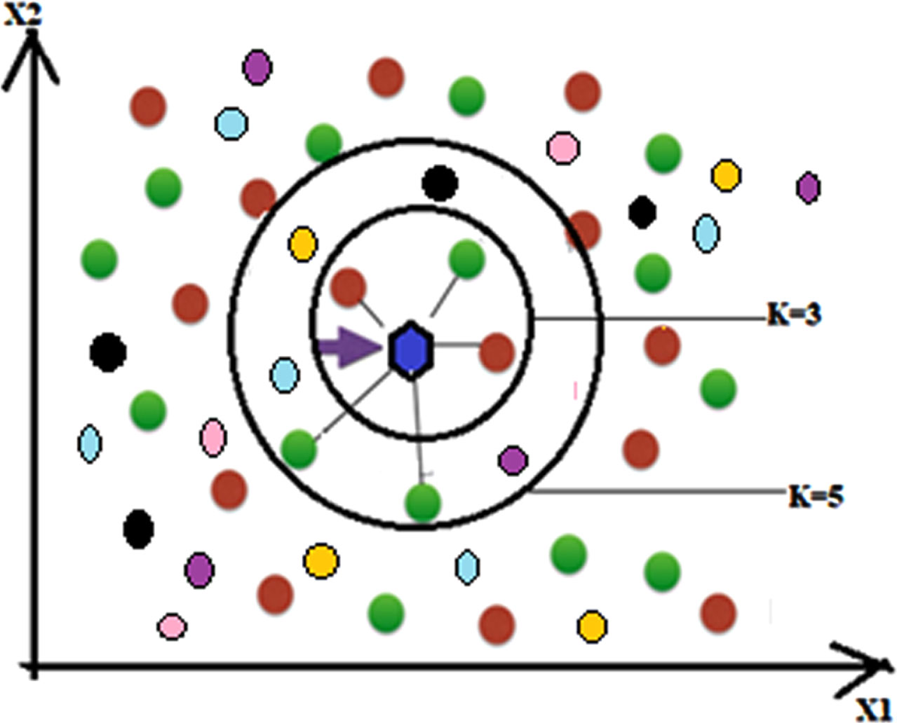
K-Nearest Neighbor.

Equation (15) gives the highest likelihood that a class will be allocated to an input x:

$P (y = j | X = x) = \frac{1}{K} \sum_{i \in A} I (y^{(i)} = j)$ (15)

$d (x, y) = \sqrt{(x_{2} - x_{1})^{2} + (y_{2} - y_{1})^{2}}$ (16)

2.3.3 LSTMs

The architecture of LSTMs is based on artificial recurrent neural networks and includes both feed forward and feedback connections. They have the capacity to process a whole data stream at once. They can function with sequences of various lengths, which is one of their most significant features. This makes them quite well-liked in the Deep Learning community. An LSTM network’s architecture is depicted in Fig. 4, and its mathematical model is described in Equations (17) through (22).

Fig. 4

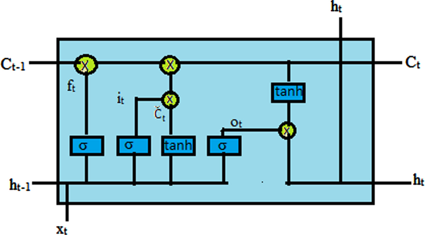
Architecture of LSTM networks.

Let us consider:

C_t, h_t: hidden layer vectors.

x_t: input vector.

b_f, b_i, b_c, b_o: bias vector.

W_f, W_i, W_c, W_o: parameter matrices.

σ, tanh: activation functions.

$f_{t} = σ (W_{f} . [h_{t - 1}, x_{t}] + b_{f})$ (17)

$i_{t} = σ (W_{i} . [h_{t - 1}, x_{t}] + b_{i})$ (18)

$o_{t} = σ (W_{o} . [h_{t - 1}, x_{t}] + b_{o})$ (19)

${\overset{ˇ}{C}}_{t} = tanh (W_{c} . [h_{t - 1}, x_{t}] + b_{c})$ (20)

$C_{t} = f_{t} ⊙ C_{t - 1} + i_{t} ⊙ \overset{ˇ}{Ct}$ (21)

$h_{t} = o_{t} ⊙ tanh (C_{t})$ (22)

The LSTM network, which accepts a series of data as input and generates predictions based on each of the data’s discrete time steps, is used to categorise the sequence data. For this network, there has been no time-domain preprocessing. A cell array containing 391 sequences of various lengths served as the network’s input, while the output—or target—is a category vector with labels 0, 1, 2, 3, 4, 5 and 6 for the ABSZ, FNSZ, GNSZ, TNSZ, TCSZ, SPSZ and CPSZ, respectively. 75 percent of the input data were used for training, while the remaining 25 percent were used to test the model. The 312 sequences from the training set were divided into numerous mini-batches and padded to have the same length. By selecting the data according to the sequence length and applying a mini-batch with a similar length, too much padding, which can occasionally negatively affect training, was avoided. The LSTM architecture with 100 hidden units and the output layer serving as the classification layer was then fed this padded input sequence. The 27-piece mini-batch was selected. The network’s output was then evaluated using test data made up of 79 sequences. The test data was sorted depending on the sequence length, just like the train data. To preserve the padding length over all sequences, the longest sequence length was used. In comparison to the test data, the projected classification data’s accuracy was calculated.

3 Result and discussion

In this paper three types of training were discussed, after feature extraction based on a) time domain pre-processing, b) frequency domain pre-processing, c) direct using raw data with 19 channels. For the first two cases, channel extraction and pre-processing were done using python, and feature selection and classification were done using the MATLAB classifier app. For all the cases feature extracted from 5 to 100 is experimented and Table 2 shown the best accuracy for number of features extracted with respect to the pre-processed methods used. To start with only features were varied keeping no hyper parameter tuning, then fine tuning of hyper parameters undertaken to improve accuracy.

Table 2
Confusion Matrix of seven seizure types using KNN

ABSZ CPSZ FNSZ GNSZ SPSZ TCSZ TNSZ

ABSZ 75 0 0 11 0 0 0

CPSZ 0 150 0 14 0 0 0

FNSZ 1 0 186 12 0 0 0

GNSZ 0 0 0 199 0 0 0

SPSZ 0 0 0 16 189 0 0

TCSZ 0 0 0 19 0 168 0

TNSZ 0 0 0 6 0 0 164

	ABSZ	CPSZ	FNSZ	GNSZ	SPSZ	TCSZ	TNSZ
ABSZ	75	0	0	11	0	0	0
CPSZ	0	150	0	14	0	0	0
FNSZ	1	0	186	12	0	0	0
GNSZ	0	0	0	199	0	0	0
SPSZ	0	0	0	16	189	0	0
TCSZ	0	0	0	19	0	168	0
TNSZ	0	0	0	6	0	0	164

3.1 Hyper parameter tuning for SVC

a) C (the regularization parameter): The C settings add a penalty for each misclassified data point. A decision boundary with a high margin must be set at the risk of additional misclassifications when the C value is low, or when the penalty for incorrectly classified points is low. On the other hand, a decision boundary with a smaller margin is produced by large C, or a high penalty for misclassification, which aims to reduce the number of misclassified samples. The penalty varies depending on how far away the decision boundary is for each misclassified example.

b) Gamma: The gamma parameter of the RBF regulates the range of influence of a single training point. Gamma’s low value indicates a large similarity radius, which leads to the grouping of more points. On the other hand, for large gamma values, the points must be quite close to one another in order to be considered in the same group. As a result, over fitting may exist in models with extremely high gamma values.

3.2 Hyperparameter tuning for KNN

The experimentation carried out for the K value varies from 1 to 29 and noted down accuracy for each k value. Out of all, it has been observed that K = 1 and K = 3 give comparatively good accuracy. Table 2, shows the best accuracy based on th e K value and features of different pre-processing techniques.

3.3 LSTM technique

A single CPU with a constant learning rate of 0.001 was the hardware resource employed. The workout lasted 725 minutes and 14 seconds. With 11 iterations per epoch, it was run for 50.

Table 3 shows the accuracy of different pre-processed techniques. For raw 19 channel data using LSTM shows 86.2% accuracy. Each seizure type accuracy is shown in the confusion matrix given in Table 2.

Table 3
Seizure type classification accuracy

Sl.No. Classifier Pre-processed Features extracted Hyperparameter tuning/ model options Accuracy obtained

1 SVC Time Domain 20 Box constraint level-2 90.41

2 Frequency domain by DFT 40 Box constraint level-2 89.4

3 Frequency domain by DCT 60 Box constraint level-2 89.4

4 Frequency domain by HT 80 – 87.5

5 KNN Time Domain 15 3-Nearest Neighbors 94.46

6 Frequency domain by DFT 30 1-Nearest Neighbors 92.72

7 Frequency domain by DCT 50 1-Nearest Neighbors 90.47

8 Frequency domain by HT 60 3-Nearest Neighbors 91.45

Sl.No.	Classifier	Pre-processed	Features extracted	Hyperparameter tuning/ model options	Accuracy obtained
1	SVC	Time Domain	20	Box constraint level-2	90.41
2	Frequency domain by DFT	40	Box constraint level-2	89.4
3	Frequency domain by DCT	60	Box constraint level-2	89.4
4	Frequency domain by HT	80	–	87.5
5	KNN	Time Domain	15	3-Nearest Neighbors	94.46
6	Frequency domain by DFT	30	1-Nearest Neighbors	92.72
7	Frequency domain by DCT	50	1-Nearest Neighbors	90.47
8	Frequency domain by HT	60	3-Nearest Neighbors	91.45

4 Conclusion

According to the study, it has been observed that, the accuracy of seven type classification from raw EEG data i.e. without any preprocessing gives accuracy of 86.2% using LSTM network whereas time-domain preprocessing enhances accuracy to 94.46% using KNN method considering K = 1. There is a sizable difference between pre-processing and no pre-processing in all respects.

On the other hand, in this study, the energy compaction property of the DFT, DCT, and HT is also employed for feature extraction and classification, which are both carried out with machine learning classifiers with feature counts varying for each of the transformations, namely FFT, DCT, and HT. Comparing the data reveals that for all sorts of transformations with various characteristics, the KNN classifier with K = 3 provides comparatively the best accuracy of 91.45% among K = 1 to K = 29.

In the future, a) dimensionality reduction techniques will be designed before each EEG sample’s energy is extracted, b) with time domain pre-processing, different classifiers can be tried out towards enhancing accuracy, c) the behaviour of same classifiers for different phases like preictal, and interictal can be explored.

5 Ethical statement

The study uses open source dataset, so no ethical clearance applicable.

Consent to participate: As a saved dataset is used, this is inapplicable.

Consent for publication: This page does not contain any information that might be used to identify the subjects.

Conflict of Interest: None of the authors must disclose any potential conflicts of interest.

Data Availability Statement: Publicly available datasets were analyzed in this study. This data can be found here: https://isip.piconepress.com/projects/tuh_eeg/html/downloads.shtml#c_tusz

References

Cura

O.K.

, Atli

S.K.

, Türe

H.S.

and Akan

, Epileptic seizure classifications using empirical mode decomposition and its derivative, BioMedical Engineering Online 19(1) (2020). DOI: 10.1186/s12938-020-0754-y.

Dutta

K.K.

, Kavya

and Swamy

S.A.

, Removal of muscle artifacts from EEG based on ensemble empirical mode decomposition and classification of Seizure using Machine LearningTechniques, IEEE- International Conference on Inventive Computing and Informatics (ICICI 2017), DOI: 10.1109/ICICI.2017.8365259.

Tatum

, Husain

, Benbadis

and Kaplan

, Handbook of EEG Interpretation. New York, NY: Demos Medical Publishing, 2007.

Yamada

and Meng

, Practical Guide for Clinical Neurophysiologic Testing: EEG. Philadelphia, PA: Lippincott Williams & Wilkins, 2009.

Wang

, Collinger

J.L.

, Degenhart

A.D.

, Tyler-Kabara

E.C.

, Schwartz

A.B.

, Moran

D.W.

, Weber

D.J.

, et al., An electrocorticographic brain interface in an individual with tetraplegia, PloS One 8(2) (2013), e55344. DOI: 10.1371/journal.pone.0055344.

Steriade

, Sperling

M.R.

, DiVentura

, Lozano

, Shellhaas

R.A.

, Kessler

S.K.

and Dlugos

, Proposal for an updated seizure classification framework in clinical trials, Epilepsia 63(3) (2022). DOI: 10.1111/epi.17120.

Vetrikani

and Christy Bobby

, Diagnosis of Epilepsy —A Systematic Review, In 2017 Third International Conference on Biosignals, Images and Instrumentation (ICBSII), Chennai: IEEE, 2017, pp. 1–5. https://doi.org/10.1109/ICBSII.2017.8082300

WHO: Media Center Epilepsy, (Fact sheet N999), (2015). http://www.who.int/mediacentre/factsheets/fs999/en/

Kusumika

K.D.

, Epilepsy is a curse: Myth or Reality-An article published by InnoHEALTH magazine digital team, (2020). https://innohealthmagazine.com/2020/issues/epilepsy-is-a-curse-myth-or-reality/

10.

Almustafa

K.M.

, Classification of epileptic seizure dataset using different machine learning algorithms, Informatics in Medicine Unlocked 21 (2020). DOI: 10.1016/j.imu.2020.100444.

11.

Arun

S.Dr.

and Dutta

K.K.

, Application of Machine Learning techniques in Electroencephalography signals, Brain & Behavior Computing, CRC Press, (c) Taylor & Francis group (2021), ISBN: 978-1-003-09288-9.

12.

Shoeibi

, Khodatars

, Ghassemi

, Jafari

, Moridian

, Alizadehsani

, Panahiazar

, Khozeimeh

, et al., Epileptic seizures detection using deep learning techniques: A review, International Journal of Environmental Research and Public Health 18(11). DOI: 10.3390/ijerph18115780.

13.

Indira

, Dutta

K.K.

, Poornima

and Swamy Bellary

S.A.

, Deep Learning Methods for Data Science, in Advanced Analytics and Deep Learning Models, JohnWiley & Sons, Inc, 2022, pp. 149–179. https://doi.org/10.1002/9781119792437.ch7

14.

Obeid

, Selesnick

and Picone

, Deep Learning Approaches for Automated Seizure Detection from Scalp Electroencephalograms, Signal Processing in Medicine and Biology, Cham: Springer, 2020, pp. 235–276.

15.

Tsiouris

K.M.

, Pezoulas

V.C.

, Zervakis

, et al., A long short-term memory deep learning network for the prediction of epileptic seizures using EEG signals, Computer Biology Medicine 99 (2018), 24–37. doi: 10.1016/j.compbiomed.2018.05.019.

16.

Dutta

K.K.

, Multi-Class Time Series Classification of EEG Signals with Recurrent Neural Networks, In 2019 9th International Conference on Cloud Computing, Data Science & Engineering (Confluence), Noida, India, 2019, pp. 337–341. DOI: 10.1109/CONFLUENCE.2019.8776889.

17.

TUH-EEG Seizure Corpus- Shah

, von Weltin

, Lopez

, McHugh

, Veloso

, Golmohammadi

, Obeid

and Picone

, The temple university hospital seizure detection corpus, Frontiers in Neuroinformatics. (2018). DOI: 10.3389/fninf.2018.00083 M. Golmohammadi, S. Ziyabari, V. Shah, et al., Gated recurrent networks for seizure detection, Proceedings of 2017 IEEE Signal Processing in Medicine and Biology Symposium, Philadelphia, PA, USA: IEEE, 2017, pp. 1–5.

18.

Dutta

K.K.

, Poornima

, Sharma

, Nair

and Ploeger

P.G.

, Applications of Recurrent Neural Network: Overview and Case Studies, in Recurrent Neural Networks, CRC Press, 2022, pp. 23–41. eBook ISBN9781003307822

19.

Dutta

K.K.

, Sridharan

and Bellary

S.A.S.

, Recurrent Neural Networks and Their Application in Seizure Classification, in Deep Learning in Visual Computing and Signal Processing, AAPAcademic Press, 2022, Hard ISBN: 9781774638705, E-Book ISBN: 9781003277224.

20.

Raghu

, Sriraam

, Temel

, Rao

S.V.

and Kubben

P.L.

, EEG based multi-class seizure type classification using convolutional neural network and transfer learning, Neural Networks 124 (2020), 202–212. DOI: 10.1016/j.neunet.2020.01.017.

21.

Segundo

, Gil-Martín

, D’Haro-Enríquez

L.F.

and Pardo

J.M.

, Classification of epileptic EEG recordings using signal transforms and convolutional neural networks, Comput Biol Med 109 (2019), 148–158.

22.

George

S.T.

, Subathra

M.S.P.

, Sairamya

N.J.

, Susmitha

and Premkumar

M.J.

, Classification of epileptic EEG signals using pso based artificial neural network and tunable-Q wavelet transform, Biocybernet Biomed Eng 40(2) (2020), 709–728.

23.

Roy

, Asif

, Tang

and Harrer

, Seizure Type Classification Using EEG Signals and Machine Learning: Setting a Benchmark, IEEE Signal Processing in Medicine and Biology Symposium (SPMB), 2020, pp. 1–6. doi: 10.1109/SPMB50085.2020.9353642.

24.

Ech-Choudany

, Scida

, Assarar

, Landré

, Bellach

and Morain-Nicolier

, Dissimilarity-based time–frequency distributions as features for epileptic EEG signal classification, Biomedical Signal Processing and Control 64 (2021). DOI: 10.1016/j.bspc.2020.102268.

25.

Yedurkar

D.P.

, Metkar

S.P.

and Stephan

, Multiresolution directed transfer function approach for segment-wise seizure classification of epileptic EEG signal, Cognitive Neurodynamics (2022), DOI: 10.1007/s11571-021-09773-z.

26.

Panigrahi

, Behera

D.K.

and Patra

K.C.

, Epileptic seizure classification of electroencephalogram signals using extreme gradient boosting classifier, Indonesian Journal of Electrical Engineering and Computer Science 25(2) (2022). DOI: 10.11591/ijeecs.v25.i2.pp884-891.

27.

Cao

, Yao

, Chen

, Sun

and Tan

, Automatic seizure classification based on domain-invariant deep representation of EEG, Frontiers in Neuroscience 15 (2021). DOI: 10.3389/fnins.2021.760987.

28.

Woodbright

, Verma

and Haidar

, Autonomous deep feature extraction based method for epileptic EEG brain seizure classification, Neurocomputing 444 (2021). DOI: 10.1016/j.neucom.2021.02.052.

29.

Jia

, Lam

H.K.

and Althoefer

, Variable weight algorithm for convolutional neural networks and its applications to classification of seizure phases and types, Pattern Recognition 121 (2022). DOI: 10.1016/j.patcog.2021.108226.

30.

Asif

, Roy

, Tang

and Harrer

, SeizureNet: Multi-Spectral Deep Feature Learning for Seizure Type Classification, Lecture Notes in Computer Science (including subseries Lecture Notes in Artificial Intelligence and Lecture Notes in Bioinformatics), 2020. DOI: 10.1007/978-3-030-66843-3_8.

31.

Dutta

K.K.

, Sharma

, Sasidharan

and Mukundan

C.S.

, Sleep monitoring wearables: Present to future, in Wearable/Personal Monitoring Devices Present to Future, Springer, Singapore, 2022, pp. 133–152. https://www.springerprofessional.de/en/sleep-monitoring-wearables-present-to-future/19797212

32.

Khosla

, Khandnor

and Chand

, EEG-based automatic multi-class classification of epileptic seizure types using recurrence plots, Expert Systems 39(5) (2022). DOI: 10.1111/exsy.12923.

33.

Purnomo

and Tjandrasa

, Epileptic seizure classification using deep batch normalization neural network, Lontar Komputer: Jurnal Ilmiah Teknologi Informasi 11(3) (2020). DOI: 10.24843/lkjiti.2020.v11.i03.p01.

34.

Ahmedt-Aristizabal

, Fernando

, Denman

, Petersson

, Aburn

M.J.

and Fookes

, Neural Memory Networks for Seizure Type Classification, Proceedings of the Annual International Conference of the IEEE Engineering in Medicine and Biology Society, EMBS, 2020. DOI: 10.1109/EMBC44109.2020.9175641.

35.

Nixon

M.S.

and Aguado

A.S.

, Images, sampling, and frequency domain processing as a book chapter in Feature Extraction & Image Processing for Computer Vision (Third Edition), 2012.

36.

Ramesh Varma

, Pavan Raju

and Prasad

M.V.R.V.

, Texture synthesis using energy compaction property of different transforms, International Journal of Computer Applications (0975 –8887) 167(8) (2017).

37.

Cooley

J.W.

and Tukey

J.W.

, An algorithm for the machine calculation of complex fourier series, Mathematics of Computation 19(90) (1965), 297–301.

38.

Johansson

, The Hilbert transform, Master Thesis Mathematics/Applied Mathematics, 2012.

39.

Bruns

, Fourier-, hilbert- and wavelet-based signal analysis: Are they really different approaches? Journal of Neuroscience Methods 137(2) (2004), 321–32. https://doi.org/10.1016/j.jneumeth.2004.03.002.

40.

Priyasad

, Fernando

, Denman

, Sridharan

and Fookes

, Interpretable seizure classification using unprocessed EEG with multi-channel attentive feature fusion, IEEE Sensors Journal 21(17) (2021). DOI: 10.1109/JSEN.2021.3090062.

Time and frequency domain pre-processing for epileptic seizure classification of epileptic EEG signals

Abstract

Keywords

1 Introduction

2 Methodology

2.2.1 Time Domain pre-processing

2.2.2 Frequency domain pre-processing

2.3 Training machine and deep learning models

2.3.1 Support Vector Classifier (SVC)

Table 2 Confusion Matrix of seven seizure types using KNN ABSZ CPSZ FNSZ GNSZ SPSZ TCSZ TNSZ ABSZ 75 0 0 11 0 0 0 CPSZ 0 150 0 14 0 0 0 FNSZ 1 0 186 12 0 0 0 GNSZ 0 0 0 199 0 0 0 SPSZ 0 0 0 16 189 0 0 TCSZ 0 0 0 19 0 168 0 TNSZ 0 0 0 6 0 0 164

3.2 Hyperparameter tuning for KNN

3.3 LSTM technique

5 Ethical statement

References

Table 2
Confusion Matrix of seven seizure types using KNN

ABSZ CPSZ FNSZ GNSZ SPSZ TCSZ TNSZ

ABSZ 75 0 0 11 0 0 0

CPSZ 0 150 0 14 0 0 0

FNSZ 1 0 186 12 0 0 0

GNSZ 0 0 0 199 0 0 0

SPSZ 0 0 0 16 189 0 0

TCSZ 0 0 0 19 0 168 0

TNSZ 0 0 0 6 0 0 164