Outlier detection for incomplete real-valued data via rough set theory and granular computing

Abstract

Outlier detection is an important topic in data mining. An information system (IS) is a database that shows relationships between objects and attributes. A real-valued information system (RVIS) is an IS whose information values are real numbers. People often encounter missing values during data processing. A RVIS with the miss values is an incomplete real-valued information system (IRVIS). Due to the presence of the missing values, the distance between two information values is difficult to determine, so the existing outlier detection rarely considered an IS with the miss values. This paper investigates outlier detection for an IRVIS via rough set theory and granular computing. Firstly, the distance between two information values on each attribute of an IRVIS is introduced, and the parameter λ to control the distance is given. Then, the tolerance relation on the object set is defined according to the distance, and the tolerance class is obtained, which is regarded as an information granule. After then, λ-lower and λ-upper approximations in an IRVIS are put forward. Next, the outlier factor of every object in an IRVIS is presented. Finally, outlier detection method for IRVIS via rough set theory and granular computing is proposed, and the corresponding algorithms is designed. Through the experiments, the proposed method is compared with other methods. The experimental results show that the designed algorithm is more effective than some existing algorithms in an IRVIS. It is worth mentioning that for comprehensive comparison, ROC curve and AUC value are used to illustrate the advantages of the proposed method.

Keywords

RST GrC IRVIS outlier detection outlier factor

1 Introduction

1.1 The relevant research work

One intuitive and popular definition of an outlier was given by Hawkins [21]: “An outlier is an observation that deviates so much from other observations as to arouse suspicions that it was generated by a different mechanism”.

As an important branch of data mining, the purpose of outlier detection is to find objects whose behavior is different from that of normal objects. Outlier detection is widely used in many fields, such as marketing [9], medical diagnosis [16], bioinformatics data [31]. In practical applications, outlier detection is an unsupervised learning problem, because outliers are few and data labeling is expensive [16].

Outlier detection strategies can also be classified as local or global based on the size of their reference set. The well-known Local Outlier Factor scoring algorithm [11] detects outliers based on local density and provides a local outlier score to each data point. For each data point, the LOF score is defined as the ratio of the average density of its neighbors to its own local density. The global unsupervised outlier identification technology may be split into three major types depending on the assumptions used in modeling outliers: clustering-based, statistics-based, and closest neighbor-based techniques. In clustering based technology [38], data that does not belong to any cluster or belongs to a very small cluster is considered as outliers. This method largely depends on the parameter setting of clustering algorithm, and its efficiency is low. In statistical-based technology [12, 41], it is assumed that the data fits a statistical model, and then a test is run to identify the data points that do not fit in the presumed model. In closest neighbor-based technology, each data point is analyzed according to its local neighborhood. The closest neighbor method is distance-based or density-based, depending on which standard is used to identify nearest neighbors and outliers [13]. In the distance-based method [30], a data point far from its nearest neighbor is regarded as an outlier. When the density of different data areas is different, the performance of these methods will be poor. The density-based method not only calculates the local density of each data point, but also calculates the local density of its adjacent points. If the density of a data point is much lower than that of its adjacent points, it is considered an outlier [33].

Granular computing (GrC), proposed by Zadeh [49], is an important tool in artificial intelligence [48]. GrC emphasizes the importance of granulation. Related work is generally combined with the fuzzy set theory [37], rough set theory (RST) [39, 40]. Lin [31] proposed a method for GrC based on neighborhood systems. Yao [44] has looked at certain GrC approaches in the context of neighborhood systems. As a computing method of information processing, GrC provides a theoretical framework for solving the problems in data mining and pattern recognition [32, 45].

Rough set theory (RST) introduced by Pawlak is a tool for handling uncertain information. This theory defines lower and upper approximations, and presents the accuracy of a set by means of two approximations. The accuracy may be applied to quantify the quality of the approximations on decision classes [39]. RST is widely used in attribute reduction [17, 43], pattern recognition [51], classification [25, 50] and data mining [14]. In recent years, RST has attracted many researchers’ attention [1 , 22], and its application is mostly related to an information system (IS). It is worth mentioning that topology plays an important role in handling an IS via RST (see [3–5 , 35]).

GrC or RST can be applied to outlier detection. In order to make up for the shortcomings of distance-based and density-based methods, outlier detection methods based on RST were also proposed. Although these methods have proved the effectiveness of RST in outlier detection. However, these methods build mathematical models based on equivalence relations, and their detection models are only applicable to nominal feature data. Numerical feature data need to be described before we use these detection models. It increases the time required for data processing and is accompanied by significant loss of information. However, this does not happen when an IRVIS is directly studied with RST and GrC.

Many scholars have developed outlier detection based on GrC or RST. Francisco et al. [19] constructed mathematical framework of outlier detection based on RST. Chen et al. [15] proposed an outlier detection algorithm based on the neighborhood rough set model. Macia-Perez et al. [36] improved outlier detection algorithm based on RST. Jiang et al. [26] presented a GrC-based outlier detection method, which uses the information table-based GrC model to detect outliers. Yuan et al. [46] studied outlier detection methods based on fuzzy rough sets (FRSs). Li [32] gave an outlier detection algorithm for categortical data using GrC. Jiang et al. [29] gave an information entropy-based approach to outlier detection. Gao et al. [20] put forward a relative granular ratio-based outlier detection method in heterogeneous data. In addition, Dey et al. [18] investigated outlier detection in social networks leveraging community structure.

1.2 Motivation and contributions

We often encounter missing values during data processing. An incomplete real-valued information system (IRVIS) means a real-valued information system (RVIS) with missing values. Due to the presence of the missing values, the distance between two information values is difficult to determine, so the existing outlier detection rarely considered an IS with the miss values.

Considering the treatment of the miss values, this paper first defines a novel distance between two information values in an IRVIS. The idea behind this distance is to introduce the probability distribution under different conditions. Then, the tolerance classes of each object under different attributes are calculated according to the distance formula in an IRVIS, and each tolerance class is regarded as an information granule. According to the upper and lower approximations, the accuracy of the approximation of an information granule is proposed to measure the uncertainty of the information granule. Moreover, the degree of outlierness of an information granule is formulated. Next, the outlier factor of each object is introduced to evaluate the likelihood of an object being an outlier, and the outlier factor detection algorithm based on RST and GrC is presented. Finally, the presented algorithm is compared to seven algorithms: CBLOF [24], DB [30], KNN [42], SEQ [28], NOOF [15], IE [27], FRGOD [47] to show some superiority. Experiments are carried out on 12 data sets downloaded from UCI, and the results shows that the presented algorithm often has the better outlier detection effect.

Based on the above research motivation, the major contributions of this paper can be summarized as follows.

(1) A novel distance between two information values in an IRVIS is defined. This distance considers the missing values.

(2) Based on RST and GrC, the outlier factor of each object is calculated. An outlier detection algorithm in an IRVIS based on RST and GrC is proposed.

(3) The experiment results illustrate the superiority of the proposed algorithm.

The workflow of this paper is depicted in Fig. 1.

Fig. 1

The workflow of this paper.

The remainder of this paper is organized as follows. Section 2 describes some preparatory work. Section 3 studies outlier detection in an IRVIS based on RST and GrC, including examples. Section 4 proposes the OF algorithm. Section 5 gives experimental results. Section 6 carries out evaluation analysis. Section 7 summaries this paper.

2 Preliminaries

We look back at binary relations and IRVISs.

Throughout this paper, O and A denote two non-empty finite sets, 2^O means the power set of O and |X| expresses the cardinality of X ∈ 2^O. Put

$O = {o_{1}, o_{2}, \dots, o_{n}}, A = {a_{1}, a_{2}, \dots, a_{m}}$ (1)

2.1 Binary relations

Recall that R is a binary relation on O whenever R ⊆ O × O. R is called

(1) Reflexive, if (o, o′) ∈ R for any o ∈ O;

(2) Symmetric, if (o, o′) ∈ R implies (o′, o) ∈ R for any o, o′ ∈ O;

(3) Transitive, if (o, o′) ∈ R and (o′, o″) ∈ R imply (o, o″) ∈ R for any o, o′, o " ∈ O.

R is said to be an equivalence relation on O, if R is reflexive, symmetric and transitive; R is called a tolerance relation on O, if R is reflexive and symmetric.

2.2 An IRVIS

Definition 2.1. [[39]] Let O be an object set and A an attribute set. Suppose that O and A are finite sets. Then the pair (O, A) is called an information system (IS), if each attribute a ∈ A determines a information function a : O → V_a, where V_a = {a (o) : o ∈ O}.

Let (O, A) be an IS. If there is a ∈ A such that * ∈ V_a, here * means a null or unknown value, then (O, A) is called an incomplete information system (IIS).

Let (O, A) be an IIS. For each a ∈ A, denote $V_{a}^{*} = {a (o) : o \in O, a (o) \neq *}$ (2) Then, $V_{a}^{*}$ means the set of all non-missing information values with respect to the attribute a.

Definition 2.2. Suppose that (O, A) is an IIS. Then (O, A) is referred to as an incomplete real-valued information system (IRVIS), if for any a ∈ A and o ∈ O, a (o) is a real number.

Example 2.3. Table 1 expresses an IRVIS (O, A), where O = {o₁, o₂, ⋯ , o₇} is an object set and A = {a₁, a₂, a₃} is an attribute set.

Table 1

An IRVIS (O, A)

	a ₁	a ₂	a ₃
o ₁	23.6	200	*
o ₂	15.5	*	10
o ₃	*	*	80
o ₄	18.3	200	10
o ₅	23.6	300	*
o ₆	*	100	40
o ₇	25.4	*	80

$V_{a_{1}}^{*} = {23.6, 15.5, 18.3, 25.4}, V_{a_{2}}^{*} = {100, 200, 300},$

$V_{a_{3}}^{*} = {10, 40, 80}$

2.3 The distance between information values with respect to each attribute in an IRVIS

∀ a ∈ A, denote $\begin{matrix} \hat{a} = \max {a (o) : o \in O, a (o) \neq *} - \min {a (o) : \\ o \in O, a (o) \neq *} \end{matrix}$ (3)

For missing data, we have the following thoughts.

1) Consider “o ≠ o′, a (o) = * , a (o′) ≠ * , a ∈ A”, because “a (o)” is treated as “do not care” condition, thus a (o) has the probability of $\frac{1}{| V_{a}^{*} |}$ to equal to one certain value of $V_{a}^{*}$ .

2) Consider “o ≠ o′, a (o) ≠ * , a (o′) = * , a ∈ A”, because “a (o′)” is treated as “do not care” condition, thus a (o′) has the probability of $\frac{1}{| V_{a}^{*} |}$ to equal to one certain value of $V_{a}^{*}$ .

3) Consider “o ≠ o′, a (o) = * , a (o′) = * , a ∈ A”, a (o) and a (o′) both have the probability of $\frac{1}{| V_{a}^{*} |}$ to equal to one certain value of $V_{a}^{*}$ , so the joint probability of a (o) and a (o′) is $\frac{1}{| V_{a}^{*} |^{2}}$ .

Definition 2.4. Let (O, A) be an IRVIS. Then ∀ o, o′ ∈ O, ∀ a ∈ A, the distance between a (o) and a (o′) is defined as follows:

d (a (o) , a (o′)) =

${\begin{matrix} 0, & o = o^{'}; \\ 1 - \frac{1}{| V_{a}^{*} |^{2}}, & o \neq o^{'}, a (o) = *, a (o^{'}) = *; \\ 1 - \frac{1}{| V_{a}^{*} |}, & o \neq o^{'}, a (o) \neq *, a (o^{'}) = *; \\ 1 - \frac{1}{| V_{a}^{*} |}, & o \neq o^{'}, a (o) = *, a (o^{'}) \neq *; \\ 0, & o \neq o^{'}, a (o) \neq *, a (o^{'}) \neq *, a (o) = a (o^{'}); \\ \frac{| a (o) - a (o^{'}) |}{\hat{a}}, & o \neq o^{'}, a (o) \neq *, a (o^{'}) \neq *, a (o) \neq a (o^{'}) . \end{matrix}$ (4)

2.4 Tolerance relations in an IRVIS

Definition 2.5. Let (O, A) be an IRVIS. Given P ⊆ A and λ ∈ [0, 1], Define

$\begin{matrix} P_{λ} = {(o, o^{'}) \in O \times O : \\ \forall a \in P, d (a (o), a (o^{'})) \leq λ} \end{matrix}$ (5) Then P_λ is called the binary relation induced by the subspace (O, P) with respect to λ.

Clearly, P_λ is a tolerance relation on O.

Denote $P_{λ} (o) = {o^{'} \in O : (o, o^{'}) \in P_{λ}}$ (6) Then P_λ (o) is referred as to the tolerance class of the object o under P_λ.

Proposition 2.6. Let (O, A) be an IRVIS. Then the following properties hold:

(1) If P ⊆ Q ⊆ A, then ∀ λ ∈ [0, 1], ∀ o ∈ O, $Q_{λ} (o) \subseteq P_{λ} (o)$ (7)

(2) If 0 ≤ λ₁ ≤ λ₂ ≤ 1, then ∀ P ⊆ A, ∀ o ∈ O, $P_{λ_{1}} (o) \subseteq P_{λ_{2}} (o)$ (8)

Proof. (1) ∀ o′ ∈ Q_λ (o), we have ∀ a ∈ Q, d (a (o) , a (o′)) ≤ λ. Since P ⊆ Q, ∀ a ∈ P, d (a (o) , a (o′)) ≤ λ. Thus o′ ∈ P_λ (o).

So Q_λ (o) ⊆ P_λ (o).

(2) ∀ o′ ∈ P_λ₁ (o), we have ∀ a ∈ P, d (a (o) , a (o′)) ≤ λ₁. Since λ₁ ≤ λ₂, ∀ a ∈ P, d (a (o) , a (o′)) ≤ λ₂. Thus o′ ∈ P_λ₂ (o).

So P_λ₁ (o) ⊆ P_λ₂ (o). □

Definition 2.7. Let (O, A) be an IRVIS. Given P ⊆ A, λ ∈ [0, 1] and X ∈ 2^O. Define $\underline{P_{λ}} (X) = {o \in O : P_{λ} (o) \subseteq X}$ (9) $\bar{P_{λ}} (X) = {o \in O : P_{λ} (o) \cap X \neq \emptyset}$ (10) Then $\underline{P_{λ}} (X)$ and $\bar{P_{λ}} (X)$ are called λ-lower approximation and λ-upper approximation of X, respectively.

Moreover, if $\underline{P_{λ}} (X) = \bar{P_{λ}} (X)$ , then X is called a exact set with respect to P_λ; otherwise, X is called a rough set with respect to P_λ.

Put $α_{P}^{λ} (X) = | \underline{P_{λ}} (X) | / | \bar{P_{λ}} (X) |$ (11) Then $α_{P}^{λ} (X)$ is called λ-accuracy of approximation of X in the subsystem (X, P).

Theorem 2.8. Let (O, A) be an IRVIS. (1) $\bar{P_{λ}} (\emptyset) = \underline{P_{λ}} (\emptyset) = \emptyset$ , $\underline{P_{λ}} (O) = \bar{P_{λ}} (O) = O$ .

(2) $\underline{P_{λ}} (X) \subseteq X \subseteq \bar{P_{λ}} (X)$ . (3) $X \subseteq Y \Rightarrow \underline{P_{λ}} (X) \subseteq \underline{P_{λ}} (Y), \bar{P_{λ}} (X) \subseteq \bar{P_{λ}} (Y)$ .

(4) If P ⊆ Q ⊆ A, then ∀ λ ∈ [0, 1], ∀ X ∈ 2^O, $\underline{P_{λ}} (X) \subseteq \underline{Q_{λ}} (X), \bar{Q_{λ}} (X) \subseteq \bar{P_{λ}} (X)$ (12)

(5) If 0 ≤ λ₁ ≤ λ₂ ≤ 1, then ∀ P ⊆ A, ∀ X ∈ 2^O, $\underline{P_{λ_{2}}} (X) \subseteq \underline{P_{λ_{1}}} (X), \bar{P_{λ_{1}}} (X) \subseteq \bar{P_{λ_{2}}} (X)$ (13)

(6) $\underline{P_{λ}} (X \cap Y) = \underline{P_{λ}} (X) \cap \underline{P_{λ}} (Y)$ ;

$\bar{P_{λ}} (X \cap Y) = \bar{P_{λ}} (X) \cup \bar{P_{λ}} (Y)$ . (7) $\underline{P_{λ}} (O - X) = O - \bar{P_{λ}} (X)$ ;

$\bar{P_{λ}} (O - X) = O - \underline{P_{λ}} (X)$ .

Proof. The conclusions are obvious according to Definition 2.5, Propositon 2.6 and Definition 2.7. □

Theorem 2.9. Let (O, A) be an IRVIS. Given

(1) If P ⊆ Q ⊆ A, then ∀ λ ∈ [0, 1], ∀ X ∈ 2^O, $α_{P}^{λ} (X) \leq α_{Q}^{λ} (X)$ (14)

(2) If 0 ≤ λ₁ ≤ λ₂ ≤ 1, then ∀ P ⊆ A, ∀ X ∈ 2^O, $α_{P}^{λ_{2}} (X) \leq α_{P}^{λ_{1}} (X)$ (15)

Proof. It can be proved by Theorem 2.8. □

3 Outliers for incomplete real-valued data based on RST and GrC

In this section, we define outliers for incomplete real-valued data via RST and GrC, and then give an example of finding the outliers.

Denote $U / P_{λ} = {P_{λ} (o) : o \in O}$ (16)

Definition 3.1. Let (O, A) be an IRVIS. Given P ⊆ A and λ ∈ [0, 1]. Let C = A - P. Suppose |C|≥2, E ⊆ C and g ∈ U/P_λ. Then (E, λ)-accuracy of approximation of the information granule g is denoted as $α_{E}^{λ} (g)$ . Define

$α_{E}^{λ} (g) = \frac{| \underline{E_{λ}} (g) |}{| \bar{E_{λ}} (g) |}$ (17)

In Definition 3.1, the approximate accuracy of information granule g to reflect the uncertainty of information granule g, and this can be interpreted as the outlier degree of g under the set of attributes E. Obviously, in IRVIS, information granule g represents the tolerance class of each object o under attribute subset P and $α_{E}^{λ} (g) \in [0, 1]$ . According to this idea, there is a concept ${DO}_{P}^{λ} (g)$ can be defined as follows.

Definition 3.2. Let (O, A) be an IRVIS. Given P ⊆ A and λ ∈ [0, 1]. Let C = A - P = {a_{k
₁}, ⋯ , a_{k
_s}}. Suppose |C|≥2 and g ∈ U/P_λ. Then (P, λ)-degree of outlierness of the information granule g is denoted as ${DO}_{P}^{λ} (g)$ . Define

${DO}_{P}^{λ} (g) = 1 - | g | \frac{α_{C}^{λ} (g) + \sum_{i = 1}^{s} (α_{C - {a_{k_{i}}}}^{λ} (g) + 1) / 2}{n (s + 1)}$ (18)

Denote ${DO}_{a}^{λ} (g) = {DO}_{{a}}^{λ} (g)$ (19)

In Definition 3.2, we use ${DO}_{P}^{λ} (g)$ to measure the outlier degree of the information granule g. $\frac{| g |}{n}$ is the weight of information granule g. For any information granule g, if the cardinality of g is less than that of other information granule, then the objects in the information granule g belong to the minority of objects, and give g a low weight to make the outlier degree of the information granule g higher. because $α_{C}^{λ} (g)$ reflects the uncertainty of g and depends on attribute subsets C. ${DO}_{P}^{λ} (g)$ use the average value of $α_{C}^{λ} (g)$ to measure the outlier degree of the information granule g. To make full advantage of the original data information it seems reasonable to calculate all possible subsets of attribute set C. However, the total number of the subsets of an attributes set C is 2^|C|, which is impractical for calculation when |C| grows large. Consequently, the accuracy of approximation is calculated only for C and C - {a_{k
_i}}.

Definition 3.3. Let (O, A) be an IRVIS. Given λ ∈ [0, 1]. Then λ-weight function of a ∈ A is defined as

$ω_{{a}}^{λ} (o) = 1 - \sqrt[3]{\frac{| {a}_{λ} (o) |}{n}}$ (20)

In Definition 3.3, {a} _λ (o) represents the tolerance class under each individual attribute a in A, that is also the information granule g containing object o. This definition illustrates the view that a few objects in the data set are more likely to be outliers. If the tolerance class of object o is small, it is more independent of other objects, so it is more likely to be an outlier.

Definition 3.4. Let (O, A) be an IRVIS with m ≥ 3. Given λ ∈ [0, 1]. Then λ-outlier factor of o ∈ O is defined as

${OF}^{λ} (o) = \frac{\sum_{j = 1}^{m} ω_{{a_{j}}}^{λ} (o) {DO}_{{a_{j}}}^{λ} ({a_{j}}_{λ} (o))}{m}$ (21)

Finally, the concept OF^λ (o) integrates all the above concepts to give the outlier factor of the object o. Again, since the total subsets of attribute set A is 2^|A|, in Definition 3.4 we only use every individual attribute a to make the subset. The outlier factor of o is directly proportional to the degree of outlierness of information granule g containing o. As a result, the larger the outlier factor of object o, the object o may belong to the minority of objects in O.

Definition 3.5. Let (O, A) be an IRVIS with m ≥ 3. Given λ, μ ∈ [0, 1]. Then o^*∈ is called (λ, μ)-outlier in an IRVIS, if OF^λ (o^*) > μ .

In this paper, the set of all (λ, μ)-outlier in an IRVIS ia denoted as $Ω_{μ}^{λ}$ .

Example 3.6. Given an IRVIS (O, A) shown in Table 1. Pick λ = 0.5. Then the tolerance class of each object is shown in Table 2.

Table 2

The tolerance class of each object

O	{a₁} _λ (o)	{a₂} _λ (o)	{a₃} _λ (o)
o ₁	{o₁, o₅, o₇}	{o₁, o₄, o₅, o₆}	{o₁}
o ₂	{o₂, o₄}	{o₂}	{o₂, o₄, o₆}
o ₃	{o₃}	{o₃}	{o₃, o₇}
o ₄	{o₂, o₄}	{o₁, o₄, o₅, o₆}	{o₂, o₄, o₆}
o ₅	{o₁, o₅, o₇}	{o₁, o₄, o₅}	{o₅}
o ₆	{o₆}	{o₁, o₄, o₆}	{o₂, o₄, o₆}
o ₇	{o₁, o₅, o₇}	{o₇}	{o₃, o₇}

Let g₁ = {a₁} _λ (o₁) , g₂ = {a₂} _λ (o₁) , g₃ = {a₃} _λ (o₁), from Table 2 we have g₁ = {o₁, o₅, o₇} , g₂ = {o₁, o₄, o₅, o₆} , g₃ = {o₁}

(1) For i = 1, 2, 3, by (3.2), the (E, λ)-accuracy of approximation is calculated as follows:

$α_{{a_{2}, a_{3}}}^{λ} (g_{1}) = \frac{| \underline{{a_{2}, a_{3}}_{λ}} (g_{1}) |}{| \bar{{a_{2}, a_{3}}_{λ}} (g_{1}) |} = \frac{| {o_{1}, o_{5}, o_{7}} |}{| {o_{1}, o_{5}, o_{7}} |} = 1,$

$α_{{a_{3}}}^{λ} (g_{1}) = \frac{| \underline{{a_{3}}_{λ}} (g_{1}) |}{| \bar{{a_{3}}_{λ}} (g_{1}) |} = \frac{| {o_{1}, o_{5}} |}{| {o_{1}, o_{3}, o_{5}, o_{7}} |} = 0.5,$

$α_{{a_{2}}}^{λ} (g_{1}) = \frac{| \underline{{a_{2}}_{λ}} (g_{1}) |}{| \bar{{a_{2}}_{λ}} (g_{1}) |} = \frac{| {o_{7}} |}{| {o_{1}, o_{4}, o_{5}, o_{6}, o_{7}} |} = 0.2,$

$α_{{a_{1}, a_{3}}}^{λ} (g_{2}) = \frac{| \underline{{a_{1}, a_{3}}_{λ}} (g_{2}) |}{| \bar{{a_{1}, a_{3}}_{λ}} (g_{2}) |} = \frac{| {o_{1}, o_{5}, o_{6}} |}{| {o_{1}, o_{2}, o_{4}, o_{5}, o_{6}} |} = 0.6,$

$α_{{a_{3}}}^{λ} (g_{2}) = \frac{| \underline{{a_{3}}_{λ}} (g_{2}) |}{| \bar{{a_{3}}_{λ}} (g_{2}) |} = \frac{| {o_{1}, o_{5}} |}{| {o_{1}, o_{2}, o_{4}, o_{5}, o_{6}} |} = 0.4,$

$α_{{a_{1}}}^{λ} (g_{2}) = \frac{| \underline{{a_{1}}_{λ}} (g_{2}) |}{| \bar{{a_{1}}_{λ}} (g_{2}) |} = \frac{| {o_{6}} |}{| {o_{1}, o_{2}, o_{4}, o_{5}, o_{6}, o_{7}} |} \approx 0.1667,$

$α_{{a_{1}, a_{2}}}^{λ} (g_{3}) = \frac{| \underline{{a_{1}, a_{2}}_{λ}} (g_{3}) |}{| \bar{{a_{1}, a_{2}}_{λ}} (g_{3}) |} = \frac{| \emptyset |}{| {o_{1}, o_{5}} |} = 0,$

$α_{{a_{2}}}^{λ} (g_{3}) = \frac{| \underline{{a_{2}}_{λ}} (g_{3}) |}{| \bar{{a_{2}}_{λ}} (g_{3}) |} = \frac{| \emptyset |}{| {o_{1}, o_{4}, o_{5}, o_{6}} |} = 0,$

$α_{{a_{1}}}^{λ} (g_{3}) = \frac{| \underline{{a_{1}}_{λ}} (g_{3}) |}{| \bar{{a_{1}}_{λ}} (g_{3}) |} = \frac{| \emptyset |}{| {o_{1}, o_{5}, o_{7}} |} = 0 .$

(2) By (3.3), the corresponding (P, λ)-degree of outlierness could be calculated accordingly:

${DO}_{{a_{1}}}^{λ} (g_{1})$

$= 1 - | g_{1} | \frac{α_{{a_{2}, a_{3}}}^{λ} (g_{1})}{n (s + 1)} + | g_{1} | \frac{(α_{{a_{3}}}^{λ} (g_{1}) + 1 + α_{{a_{2}}}^{λ} (g_{1}) + 1) / 2}{n (s + 1)}$

≈0.6643,

${DO}_{{a_{2}}}^{λ} (g_{2})$

$= 1 - | g_{2} | \frac{α_{{a_{1}, a_{3}}}^{λ} (g_{2})}{n (s + 1)} + | g_{2} | \frac{(α_{{a_{3}}}^{λ} (g_{2}) + 1 + α_{{a_{1}}}^{λ} (g_{2}) + 1) / 2}{n (s + 1)}$

≈0.6413,

${DO}_{{a_{3}}}^{λ} (g_{3})$

$= 1 - | g_{3} | \frac{α_{{a_{1}, a_{2}}}^{λ} (g_{3})}{n (s + 1)} + | g_{2} | \frac{(α_{{a_{2}}}^{λ} (g_{3}) + 1 + α_{{a_{1}}}^{λ} (g_{3}) + 1) / 2}{n (s + 1)}$

≈0.9524 .

(3) By (3.5), the λ-weight function by Definition 3.3 is calculated as follows:

$ω_{{a_{1}}}^{λ} (o_{1}) = 1 - \sqrt[3]{\frac{| {a_{1}}_{λ} (o_{1}) |}{n}} = 1 - \sqrt[3]{\frac{| {o_{1}, o_{5}, o_{7}} |}{n}} = 1 - \sqrt[3]{\frac{3}{7}} \approx 0.2461,$

$ω_{{a_{2}}}^{λ} (o_{1}) = 1 - \sqrt[3]{\frac{| {a_{2}}_{λ} (o_{1}) |}{n}} = 1 - \sqrt[3]{\frac{| {o_{1}, o_{4}, o_{5}, o_{6}} |}{n}} = 1 - \sqrt[3]{\frac{4}{7}} \approx 0.1702,$

$ω_{{a_{3}}}^{λ} (o_{1}) = 1 - \sqrt[3]{\frac{| {a_{3}}_{λ} (o_{1}) |}{n}} = 1 - \sqrt[3]{\frac{| {o_{1}} |}{n}} = 1 - \sqrt[3]{\frac{1}{7}} \approx 0.4772 .$

(4) By (3.6), the λ-outlier factor proposed in Definition 3.4 can be calculated as follows:

O F^{λ} (o_{1}) = \frac{\sum_{j = 1}^{m} ω_{a_{j}}^{λ} (o_{1}) D O_{a_{j}}^{λ} ({a_{j}}_{λ} (o_{1}))}{m} = \frac{0.2461 \times 06643 + 01702 \times 06413 + 04772 \times 0.9524}{3} \approx 02424

(5) We can get all λ-outlier factors of every objects:

OF^λ (o₁) =0.2424, OF^λ (o₂) =0.3013, OF^λ (o₃) =0.3656, OF^λ (o₄) =0.1862, OF^λ (o₅) =0.2681, OF^λ (o₆) =0.2651, OF^λ (o₇) =0.2838.

Given μ = 0.35, we have

O F^{λ} (o_{4}) < O F^{λ} (o_{1}) < O F^{λ} (o_{6}) < O F^{λ} (o_{5}) < O F^{λ} (o_{7}) < O F^{λ} (o_{2}) < μ < O F^{λ} (o_{3}),

Only o₃ has an OF^λ higher than the threshold μ, and is thus taken as outlier according to Definition 3.5.

4 Outlier detection algorithms

This section proposes outlier detection algorithms and analyses their time complexity.

Given an IRVIS (O, A), our method is represented in Algorithms 1 and 2. Algorithm 1 calculates the tolerance class of each object under each attribute to obtain the divided information granules. Algorithm 2 calculates the outlier set.

The time complexity for Algorithm 1 is as follows. In step 4, the time complexity for calculating the d (a (o) , a (o′)) is O (|P| × |O|²), where |P| stands for the number of elements in set P. In step 6, calculate the tolerance class of the object o under attribute set P, which is equivalent to the intersection operation of multiple sets, and its time complexity is O (|P| × |O|). Therefore, the time complexity of the whole algorithm 1 is O (|P| × |O|² + |P| × |O|), so in the worst case, the time complexity of algorithm 1 is O (|P| × |O|²).

For Algorithm 2, calculation costs for Steps 5 and 7 are O (|O| × |A|), O (|O| × |A| × (|A|-1)) according to Definition 3.1, and those for Steps 9, 10 and 12 are O (|O| × |A|) , O (|O| × |A|) , O (|O|) , according to formula 3.3, 3.5 and 3.6, respectively. Thus, the total time complexity for Algorithm 2 amounts to O (3 × |O| × |A| + |O| × |A| × (|A|-1) + O (|O|). In the worst case, the time complexity of algorithm 2 is O (|O| × |A|²).

Algorithm 1
Computing P_λ (o)

Input: An IRVIS (O, A), a threshold λ ∈ [0, 1], P ⊆ A and o ∈ O.

1: Output: The tolerance class P_λ (o).

2: P_λ (o)← ∅

3: for a ∈ P do

4: for o, o′ ∈ O do

5: Calculate d (a (o) , a (o′)) by formula (2.4)

6: if d (a (o) , a (o′)) ≤ λ then

7: P_λ (o) ← P_λ (o) ∪ {o′}

8: end if

9: end for

10: end for

return P_λ (o).
Algorithm 2
Calculating the outlier set

Input: An IRVIS (O, A) and two thresholds λ, μ ∈ [0, 1].

1:

Output: Calculating $Ω_{μ}^{λ}$ .

2: $Ω_{μ}^{λ} \leftarrow \emptyset$

3: for o ∈ O do

4: for a ∈ A

5: Obtain tolerance class a_λ (o) by Algorithm 1

6: Calculate $α_{A - {a}}^{λ} (a_{λ} (o))$ by formula (3.2)

7: for b ∈ A - {a} do

8: Calculate $α_{A - {a, b}}^{λ} (a_{λ} (o))$ by formula (3.2)

9: end for

10: Calculate ${DO}_{a}^{λ} (a_{λ} (o))$ by formula (3.3)

11: Calculate $ω_{a}^{λ} (o)$ by formula (3.5)

12: end for

13: Calculate OF^λ (o) by formula (3.6)

14: if OF^λ (o) >μ then

15: $Ω_{μ}^{λ} \leftarrow Ω_{μ}^{λ} \cup {o}$

16: end if

17: end for

18: return $Ω_{μ}^{λ}$ .
5 Experimental analyses

This section gives experimental analyses.

5.1 Experimental setup

The experiments in this section are carried out on a computer equipped with Inter Corei5-7200U processor, frequency of 2.50 GHz, storage of 2.70 GHz and memory of 12 GB. The operating system is Windows 10. The experiments are developed with Python 3.8. Python IDE is Pycharm 2020.2.1.

The performance of all outlier detection algorithms in this section is evalued by the metric proposed by Aggarwal [10]. First, it is clear that those objects belonging to rare classes in each data set are considered outliers. If the given outlier detection algorithm works well, it is expected that these outliers to be over represented in the detected object set.

In other words, for each algorithm, we first calculate the outlier degree of each object in the data set, then arrange the outlier degree in descending order, and set an appropriate threshold. All objects with outlier degree greater than the threshold are selected to become a set of objects to be tested. If there are more objects belonging to rare classes(abnormal classes) in the object set to be tested, the better the performance. It is expected that the outlier degree of objects in all rare classes to be as high as possible, so the easier it is to detect, which means the better the performance of the algorithm.

The appropriate threshold μ mentioned above is obtained according to the proportion of rare classes in each data set. The specific assignment operations will be introduced in different data sets

5.2 Data sets

Twelve data sets from UCI Machine Learning Repository are used: Bone marrow transplant children Data Set, Breast Cancer Wisconsin (Original) Data Set, Breast Cancer Wisconsin (Prognostic) Data Set, Computer Hardware Data Set, Glass Identification Data Set, HCV Data Set, CSM 2014 and 2015 Data Set, Airfoil Self-Noise Data Set, Climate Model Simulation Crashes Data Set, Winequality-Red Data Set, Thoracic Surgery Data Set, Blood Transfusion Service Center Data Set.

The attribute values of these data sets are real-values. There are missing values in the six data sets: Bone marrow transplant children Data Set, Breast Cancer Wisconsin (Original) Data Set, Breast Cancer Wisconsin (Prognostic) Data Set, HCV Data Set, CSM 2014 and 2015 Data Set and Winequality-Red Data Set. Other data sets need data missing preprocessing to achieve the purpose of studying IRVIS. And the missing rate parameters are analyzed in the process of data missing preprocessing.

Concretely, a real-valued data set D could be regarded as an IS (O, A) (see Definition 2.1). The determinate value of object o under attribute a is a (o); while the missing value of object o under attribute a is *. This way the data set is transformed into an IRVIS.

Each data set contains a small fraction of objects that is deemed as “rare class”, and such classification usually involves some semantics under certain context, such as in the background of wing noise tests the instances of high noise are taken as outliers.

Table 3 summarizes the data set used in this experiment. Firstly, all data sets without missing attributes are preprocessed by randomly missing attribute values. Then, in order to better conduct outlier detection experiments, it is necessary to treat abnormal classes as minority classes and normal classes as majority classes. Therefore, abnormal objects only make up a small portion of the entire data set. Furthermore, if the data set has an ID attribute, although it is a real value attribute, it is not considered. As shown in Table 3, the “data sets” column represents the name of each corresponding data set; The “dimensions” column represents the size of the corresponding data set attribute set; The “objects” column represents the size of the experimental object set corresponding to each data set; The “outlier ratio” column represents the proportion of abnormal objects in each data set.

Table 3
Statistics of the public benchmark data sets

data sets dimensions objects outlier ratio

1 Bone marrow transplant: children 37 158 35.44%

2 Breast Cancer Wisconsin (Original) 10 699 34.48%

3 Breast Cancer Wisconsin (Prognostic) 34 198 23.74%

4 Computer Hardware 10 209 5.74%

5 Glass Identification 9 85 10.59%

6 HCV 13 615 12.20%

7 CSM 2014 and 2015 13 231 9.09%

8 Airfoil Self-Noise 6 1503 5.26%

9 Climate Model Simulation Crashes 19 540 8.52%

10 Winequality-Red 12 862 0.81%

11 Thoracic Surgery 17 470 14.89%

12 Blood Transfusion Service Center 5 748 23.80%

	data sets	dimensions	objects	outlier ratio
1	Bone marrow transplant: children	37	158	35.44%
2	Breast Cancer Wisconsin (Original)	10	699	34.48%
3	Breast Cancer Wisconsin (Prognostic)	34	198	23.74%
4	Computer Hardware	10	209	5.74%
5	Glass Identification	9	85	10.59%
6	HCV	13	615	12.20%
7	CSM 2014 and 2015	13	231	9.09%
8	Airfoil Self-Noise	6	1503	5.26%
9	Climate Model Simulation Crashes	19	540	8.52%
10	Winequality-Red	12	862	0.81%
11	Thoracic Surgery	17	470	14.89%
12	Blood Transfusion Service Center	5	748	23.80%

5.3 Experimental result

A brief comparison between all the outlier detection algorithms is shown in Table 4.

Table 4
Comparison among outlier detection methods

Method Meaning Advantage Disadvantage

OF Incomplete real-valued outlier factor method Deal with missing values effectively;high performance High time complexity

CBLOF Finding cluster based local outlier factor Deal with local outliers Low performance

DB Distance-based detection Relatively simple Unstable performance

KNN k-nearest neighbor Simple implementation High time complexity

SEQ Sequence based High performance Discretization pretreatment for numeric data

NOOF Neighborhood detection Relatively simple Underuse of data information

IE Information entropy based Relative entropy needs to be considered Unstable performance

FRGOD Fuzzy rough granules based Deal with mixed attribute data Relatively high time and spatial complexity

Method	Meaning	Advantage	Disadvantage
OF	Incomplete real-valued outlier factor method	Deal with missing values effectively;high performance	High time complexity
CBLOF	Finding cluster based local outlier factor	Deal with local outliers	Low performance
DB	Distance-based detection	Relatively simple	Unstable performance
KNN	k-nearest neighbor	Simple implementation	High time complexity
SEQ	Sequence based	High performance	Discretization pretreatment for numeric data
NOOF	Neighborhood detection	Relatively simple	Underuse of data information
IE	Information entropy based	Relative entropy needs to be considered	Unstable performance
FRGOD	Fuzzy rough granules based	Deal with mixed attribute data	Relatively high time and spatial complexity

Figure 2 shows the scatter plot distribution of all data sets, with the abscissa representing the object number and the ordinate representing the size of the outlier factor calculated by the OF outlier detection algorithm in each scatter plot. The red dot represents the true outlier, and the red dashed line represents the corresponding threshold horizontal line under the data set. The calculation method is to first calculate the outlier factor of each object based on the designed algorithm, and then sort it in descending order according to the value of the outlier factor. Under the premise of each data set, there is a outlier ratio (see Table 3). The size of outlier factor in descending order of outlier ratio is taken as the threshold horizontal line.

Fig. 2

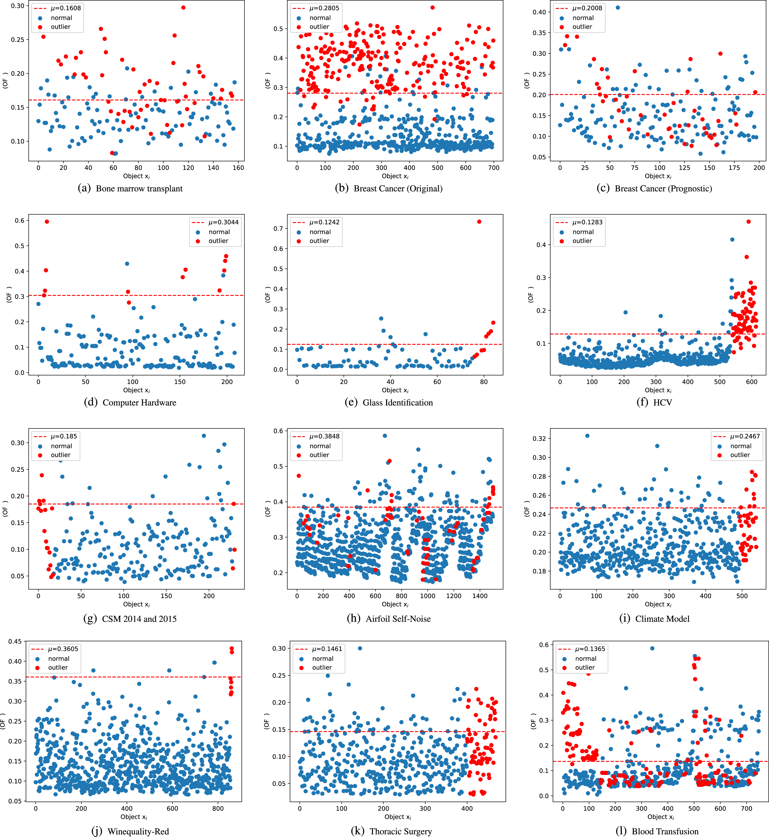
Scatter chart results.

Figure 3 shows the detection rate comparison chart of all data sets. The proposed algorithm (OF) has excellent outlier detection effect on the four data sets of Breast Cancer (Original), Computer Hardware, HCV and Winequality-Red. The detection rate line chart also shows that the front is almost the same slope upward, and then becomes stable until all outliers are found. For example, among the first 80 objects detected after sorting by outlier factors in descending order on the Breast Cancer (Original) data set, they are actually all abnormal points. At this time, the detection rate reaches 100%. If you add another 20 objects and take the first 100 objects, the number of real outliers is 98, which is equivalent to misjudging only two objects. In the comparison chart of the detection rate of the remaining data sets, it can also be clearly seen that the proposed algorithm (OF) is always in the first echelon, with either the front detection rate leading or the back detection rate leading. Overall, the proposed algorithm is better than the existing algorithms.

Fig. 3

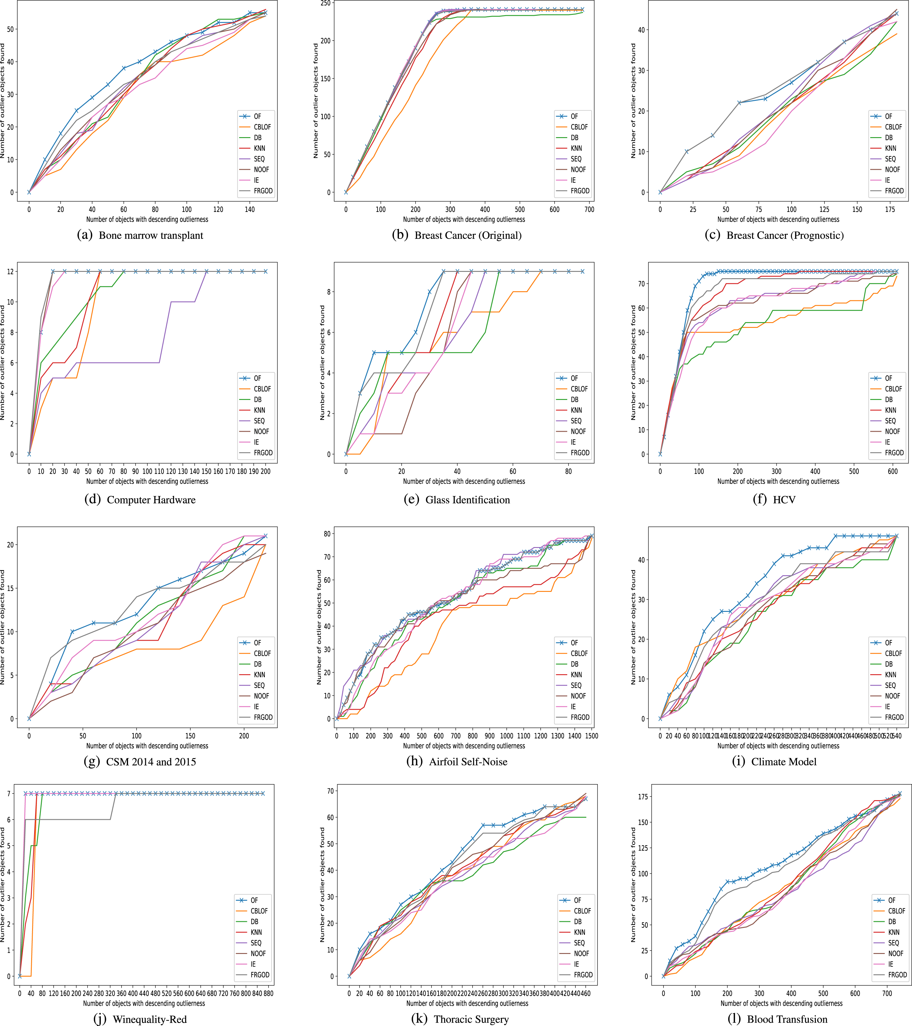
Comparison results of detection rate.

The following is a comparison table of different algorithm detection rates for 12 data sets. Each table compares the experimental results of OF algorithm, CBLOF algorithm, DB algorithm, KNN algorithm, SEQ algorithm, NOOF algorithm, IE algorithm, and FRGOD algorithm at different detection stages. Bold font represents the best detection effect at the current detection stage. Here, the “top ratio” is ratio of the number of objects specified as top-k outliers to that of the objects in the data set. The “coverage” is ratio of the number of detected rare classes to that of the rare classes in the data set.

Bone marrow transplant data set. The Bone marrow transplant data set from UCI Machine Learning Repository includes 187 objects and 37 attributes. In order to make up only a small portion of the entire data set, the rare classes were processed according to the method in reference [23]. Specifically, the number of some rare classes was removed, resulting in a total experimental data set size of 158. The last attribute is the decision attribute, which represents survival status (0 - alive, 1 - dead). In this data set, those with a survival state of “1” are considered rare classes in the data set. Because these few objects only account for 35.44% of the total data set (see Table 3). According to the percentage of rare class and the calculation method of threshold μ, the threshold μ = 0.1608 in the data set is obtained (see Fig. 2(a)). It can be seen from Table 5 that among the top ten objects that are most likely to become real outliers calculated by different algorithms, OF algorithm detects 10 real outliers. In contrast, CBLOF algorithm detects 5 real outliers, DB algorithm detects 7 real outliers, KNN algorithm detects 7 real outliers, SEQ algorithm detects 6 real outliers, NOOF algorithm detects 6 real outliers, IE algorithm detects 5 real outliers, FRGDO algorithm detects 8 real outliers. In the subsequent comparison, OF algorithm proposed in this paper has always been the best outlier detection rate.

Table 5

Experimental results in Bone marrow transplant data set

Top ratio(%)	Number of rare classes included(Coverage(%))
(Number of objects)	OF	CBLOF	DB	KNN	SEQ	NOOF	IE	FRGOD
0.06(10)	10(17.8571)	5(8.9286)	7(12.5)	7(12.5)	6(10.7143)	6(10.7143)	5(8.9286)	8(14.2857)
0.13(20)	18(32.1429)	7(12.5)	10(17.8571)	11(19.6429)	12(21.4286)	13(23.2143)	10(17.8571)	16(28.5714)
0.19(30)	25(44.6429)	13(23.2143)	16(28.5714)	16(28.5714)	18(32.1429)	18(32.1429)	15(26.7857)	22(39.2857)
0.25(40)	29(51.7857)	18(32.1429)	21(37.5)	20(35.7143)	19(33.9286)	23(41.0714)	23(41.0714)	25(44.6429)
0.32(50)	33(58.9286)	22(39.2857)	23(41.0714)	25(44.6429)	27(48.2143)	27(48.2143)	27(48.2143)	29(51.7857)
0.38(60)	38(67.8571)	29(51.7857)	30(53.5714)	30(53.5714)	32(57.1429)	31(55.3571)	29(51.7857)	33(58.9286)
0.44(70)	40(71.4286)	36(64.2857)	35(62.5)	35(62.5)	36(64.2857)	36(64.2857)	33(58.9286)	35(62.5)
0.51(80)	43(76.7857)	40(71.4286)	42(75.0)	39(69.6429)	39(69.6429)	39(69.6429)	35(62.5)	40(71.4286)
0.57(90)	46(82.1429)	40(71.4286)	45(80.3571)	44(78.5714)	43(76.7857)	43(76.7857)	40(71.4286)	43(76.7857)
0.63(100)	48(85.7143)	41(73.2143)	48(85.7143)	48(85.7143)	45(80.3571)	45(80.3571)	44(78.5714)	45(80.3571)

Breast Cancer Wisconsin (Original) Data Set. The data set includes 699 objects and 10 attributes. The last attribute is the decision attribute, which divides all objects into “benign” and “malignant”, in which “malignant” objects only account for 34.48% of the whole data set (see Table 3). Regarding “malignant” class as a rare class, according to the percentage of rare class and the calculation method of threshold μ, it can get the threshold μ = 0.2805 in this data set (see Fig. 2(b)). As shown in Table 6, OF algorithm, SEQ algorithm, NOOF algorithm, IE algorithm and FRGOD algorithm are all very good in the initial detection stage, and then OF algorithm is slightly inferior to the IE algorithm in the whole detection process.

Table 6

Experimental results in Breast Cancer Wisconsin (Original) data set

Top ratio(%)	Number of rare classes included(Coverage(%))
(Number of objects)	OF	CBLOF	DB	KNN	SEQ	NOOF	IE	FRGOD
0.03(20)	20(8.2988)	9(3.7344)	18(7.4689)	18(7.4689)	20(8.2988)	20(8.2988)	20(8.2988)	20(8.2988)
0.06(40)	40(16.5975)	19(7.8838)	38(15.7676)	35(14.5228)	40(16.5975)	40(16.5975)	40(16.5975)	40(16.5975)
0.09(60)	60(24.8963)	35(14.5228)	56(23.2365)	52(21.5768)	59(24.4813)	60(24.8963)	59(24.4813)	60(24.8963)
0.11(80)	80(33.195)	47(19.5021)	75(31.1203)	68(28.2158)	79(32.7801)	80(33.195)	79(32.7801)	80(33.195)
0.14(100)	98(40.6639)	65(26.971)	95(39.4191)	86(35.6846)	98(40.6639)	98(40.6639)	98(40.6639)	98(40.6639)
0.17(120)	118(48.9627)	80(33.195)	115(47.7178)	105(43.5685)	117(48.5477)	115(47.7178)	118(48.9627)	118(48.9627)
0.2(140)	138(57.2614)	95(39.4191)	135(56.0166)	123(51.0373)	135(56.0166)	132(54.7718)	138(57.2614)	138(57.2614)
0.23(160)	154(63.9004)	107(44.3983)	155(64.3154)	141(58.5062)	153(63.4855)	149(61.8257)	158(65.5602)	154(63.9004)
0.26(180)	172(71.3693)	122(50.6224)	174(72.1992)	157(65.1452)	170(70.5394)	165(68.4647)	175(72.6141)	172(71.3693)
0.29(200)	190(78.8382)	141(58.5062)	193(80.083)	177(73.444)	190(78.8382)	181(75.1037)	193(80.083)	190(78.8382)

Breast Cancer Wisconsin (Diagnostic) Data Set. The data set has 198 objects and 34 attributes. The last attribute is decision attribute, which divides the whole data set into “M” (malignant) and “B” (benign). The “M” (malignant) class is regarded as a rare class in the experiment, with a proportion of 23.74% as shown in Table 3. According to the proportion of rare class, it can be calculated that the threshold μ under this data set is 0.2008 (see Fig. 2(c)). As shown in Table 7, all algorithms have poor detection performance, but relatively speaking, the OF algorithm and FRGOD algorithm perform slightly better. For example, in these two algorithms, the 20 objects that are most likely to become outliers, 10 true outliers are detected.

Table 7

Experimental results in Breast Cancer Wisconsin (Diagnostic) data set

Top ratio(%)	Number of rare classes included(Coverage(%))
(Number of objects)	OF	CBLOF	DB	KNN	SEQ	NOOF	IE	FRGOD
0.1(20)	10(21.2766)	3(6.383)	5(10.6383)	3(6.383)	3(6.383)	4(8.5106)	4(8.5106)	10(21.2766)
0.2(40)	14(29.7872)	6(12.766)	7(14.8936)	8(17.0213)	6(12.766)	6(12.766)	5(10.6383)	14(29.7872)
0.3(60)	22(46.8085)	9(19.1489)	11(23.4043)	12(25.5319)	13(27.6596)	12(25.5319)	8(17.0213)	22(46.8085)
0.4(80)	23(48.9362)	16(34.0426)	17(36.1702)	18(38.2979)	18(38.2979)	18(38.2979)	12(25.5319)	24(51.0638)
0.51(100)	27(57.4468)	22(46.8085)	23(48.9362)	22(46.8085)	24(51.0638)	22(46.8085)	20(42.5532)	28(59.5745)
0.61(120)	32(68.0851)	26(55.3191)	27(57.4468)	27(57.4468)	31(65.9574)	30(63.8298)	26(55.3191)	32(68.0851)
0.71(140)	37(78.7234)	31(65.9574)	29(61.7021)	32(68.0851)	37(78.7234)	33(70.2128)	33(70.2128)	37(78.7234)
0.81(160)	40(85.1064)	35(74.4681)	34(72.3404)	39(82.9787)	41(87.234)	39(82.9787)	40(85.1064)	40(85.1064)
0.91(180)	44(93.617)	39(82.9787)	42(89.3617)	44(93.617)	44(93.617)	45(95.7447)	42(89.3617)	44(93.617)

Computer Hardware Data Set. Computer hardware data set from the UCI Machine Learning Repository includes 209 objects and 10 attributes. The final attribute is the decision attribute, which represents the estimated relative performance score. Under this data set, all objects with a performance score greater than 350 are considered as objects in the rare class. Because these objects only account for 5.74% of the total data set (see Table 3), based on the percentage of rare classes in the total data set and the calculation method of threshold μ, the threshold μ calculated in computer hardware data set is 0.3044 (see Fig. 2(d)). It can be seen from Table 8 that OF, NOOF, IE and FRGOD algorithms all have good outlier detection performance.

Table 8

Experimental results in Computer Hardware data set

Top ratio(%)	Number of rare classes included(Coverage(%))
(Number of objects)	OF	CBLOF	DB	KNN	SEQ	NOOF	IE	FRGOD
0.05(10)	8(66.6667)	3(25.0)	6(50.0)	5(41.6667)	4(33.3333)	8(66.6667)	8(66.6667)	9(75.0)
0.1(20)	12(100.0)	5(41.6667)	7(58.3333)	6(50.0)	5(41.6667)	12(100.0)	11(91.6667)	12(100.0)
0.14(30)	12(100.0)	5(41.6667)	8(66.6667)	6(50.0)	5(41.6667)	12(100.0)	12(100.0)	12(100.0)
0.19(40)	12(100.0)	5(41.6667)	9(75.0)	7(58.3333)	6(50.0)	12(100.0)	12(100.0)	12(100.0)
0.24(50)	12(100.0)	8(66.6667)	10(83.3333)	10(83.3333)	6(50.0)	12(100.0)	12(100.0)	12(100.0)
0.29(60)	12(100.0)	12(100.0)	11(91.6667)	12(100.0)	6(50.0)	12(100.0)	12(100.0)	12(100.0)
0.33(70)	12(100.0)	12(100.0)	11(91.6667)	12(100.0)	6(50.0)	12(100.0)	12(100.0)	12(100.0)
0.38(80)	12(100.0)	12(100.0)	12(100.0)	12(100.0)	6(50.0)	12(100.0)	12(100.0)	12(100.0)
0.43(90)	12(100.0)	12(100.0)	12(100.0)	12(100.0)	6(50.0)	12(100.0)	12(100.0)	12(100.0)
0.48(100)	12(100.0)	12(100.0)	12(100.0)	12(100.0)	6(50.0)	12(100.0)	12(100.0)	12(100.0)

Glass Identification Data Set. Glass Identification data set from the UCI machine learning repository includes 214 objects with 9 attributes and can be divided into 6 categories. Due to the small difference in the number of categories, 85 of them were selected as the experimental data set. The decision category of “tableware glass” is considered a rare category, as it accounts for only 10.59% of the entire data set (see Table 3). According to the percentage of rare category in the total data set and the calculation method of threshold μ, the threshold μ calculated in computer hardware data set is 0.1242 (see Fig. 2(e)). It can be seen from Table 9 that the detection performance of the OF algorithm is the best throughout the entire detection stage.

Table 9

Experimental results in Glass Identification data set

Top ratio(%)	Number of rare classes included(Coverage(%))
(Number of objects)	OF	CBLOF	DB	KNN	SEQ	NOOF	IE	FRGOD
0.06(5)	3(33.3333)	0(0.0)	2(22.2222)	1(11.1111)	1(11.1111)	1(11.1111)	1(11.1111)	3(33.3333)
0.12(10)	5(55.5556)	1(11.1111)	3(33.3333)	1(11.1111)	2(22.2222)	1(11.1111)	1(11.1111)	4(44.4444)
0.18(15)	5(55.5556)	5(55.5556)	5(55.5556)	3(33.3333)	4(44.4444)	1(11.1111)	3(33.3333)	4(44.4444)
0.24(20)	5(55.5556)	5(55.5556)	5(55.5556)	4(44.4444)	4(44.4444)	1(11.1111)	3(33.3333)	4(44.4444)
0.29(25)	6(66.6667)	5(55.5556)	5(55.5556)	5(55.5556)	4(44.4444)	3(33.3333)	4(44.4444)	5(55.5556)
0.35(30)	8(88.8889)	5(55.5556)	5(55.5556)	5(55.5556)	4(44.4444)	4(44.4444)	4(44.4444)	7(77.7778)
0.41(35)	9(100.0)	6(66.6667)	5(55.5556)	7(77.7778)	5(55.5556)	5(55.5556)	5(55.5556)	9(100.0)
0.47(40)	9(100.0)	6(66.6667)	5(55.5556)	9(100.0)	6(66.6667)	8(88.8889)	7(77.7778)	9(100.0)
0.53(45)	9(100.0)	7(77.7778)	5(55.5556)	9(100.0)	7(77.7778)	9(100.0)	9(100.0)	9(100.0)
0.59(50)	9(100.0)	7(77.7778)	6(66.6667)	9(100.0)	9(100.0)	9(100.0)	9(100.0)	9(100.0)

HCV Data Set. This experimental data set consists of 615 objects and 13 attributes. The last column of the attribute set is the decision column, which categorizes the entire data set, the “cirrhosis” as a rare class. This rare class only accounts for 12.20% of the entire data set (see Table 3). According to the ratio of rare class to the entire data set and the calculation method of the threshold μ, the threshold μ under this data set is 0.1283 (see Fig. 2(f)). As shown in Table 10 below, in the early comparison of anomaly detection rates, the OF anomaly detection algorithm was slightly inferior to CBLOF, DB, and KNN anomaly detection algorithms. However, in the subsequent detection stages, the OF anomaly detection algorithm was in a leading position.

Table 10

Experimental results in HCV data set

Top ratio(%)	Number of rare classes included(Coverage(%))
(Number of objects)	OF	CBLOF	DB	KNN	SEQ	NOOF	IE	FRGOD
0.02(10)	7(9.3333)	9(12.0)	9(12.0)	9(12.0)	7(9.3333)	7(9.3333)	7(9.3333)	7(9.3333)
0.03(20)	16(21.3333)	17(22.6667)	16(21.3333)	18(24.0)	15(20.0)	15(20.0)	15(20.0)	16(21.3333)
0.05(30)	23(30.6667)	27(36.0)	21(28.0)	26(34.6667)	21(28.0)	24(32.0)	21(28.0)	23(30.6667)
0.07(40)	32(42.6667)	32(42.6667)	29(38.6667)	32(42.6667)	31(41.3333)	32(42.6667)	27(36.0)	32(42.6667)
0.08(50)	42(56.0)	38(50.6667)	35(46.6667)	38(50.6667)	38(50.6667)	40(53.3333)	31(41.3333)	40(53.3333)
0.1(60)	50(66.6667)	47(62.6667)	37(49.3333)	44(58.6667)	43(57.3333)	46(61.3333)	37(49.3333)	49(65.3333)
0.11(70)	59(78.6667)	50(66.6667)	37(49.3333)	51(68.0)	48(64.0)	51(68.0)	42(56.0)	54(72.0)
0.13(80)	64(85.3333)	50(66.6667)	39(52.0)	55(73.3333)	51(68.0)	55(73.3333)	47(62.6667)	60(80.0)
0.15(90)	69(92.0)	50(66.6667)	40(53.3333)	57(76.0)	53(70.6667)	55(73.3333)	50(66.6667)	62(82.6667)
0.16(100)	71(94.6667)	50(66.6667)	41(54.6667)	59(78.6667)	54(72.0)	56(74.6667)	52(69.3333)	64(85.3333)

CSM 2014 and 2015 Data Set. The experimental data set consists of 231 objects and 13 attributes. The last column of the attribute set is the decision column, which represents the rating of the movie. If the experiment is interested in movies with low ratings, then consider movies with ratings below 5 as the rare class. This rare class only accounts for 9.09% of the entire data set (see Table 3). According to the ratio of rare class to the entire data set and the calculation method of the threshold μ, the threshold μ under this data set is 0.185 (see Fig. 2(g)). As shown in Table 11 below, the performance of all outlier detection algorithms is not very good in this data set. For example, when each outlier detection algorithm calculates that the top 20 are most likely to become outlier objects, the FRGOD outlier detection algorithms with the best detection rate currently only detect 7 actual outlier. However, compared to other outlier detection algorithms, the OF outlier detection algorithm has relatively better detection performance.

Table 11

Experimental results in CSM 2014 and 2015 data set

Top ratio(%)	Number of rare classes included(Coverage(%))
(Number of objects)	OF	CBLOF	DB	KNN	SEQ	NOOF	IE	FRGOD
0.09(20)	4(19.0476)	3(14.2857)	3(14.2857)	4(19.0476)	3(14.2857)	2(9.5238)	3(14.2857)	7(33.3333)
0.17(40)	10(47.619)	4(19.0476)	5(23.8095)	4(19.0476)	4(19.0476)	3(14.2857)	7(33.3333)	9(42.8571)
0.26(60)	11(52.381)	6(28.5714)	6(28.5714)	6(28.5714)	6(28.5714)	7(33.3333)	9(42.8571)	10(47.619)
0.35(80)	11(52.381)	7(33.3333)	8(38.0952)	8(38.0952)	8(38.0952)	8(38.0952)	9(42.8571)	11(52.381)
0.43(100)	12(57.1429)	8(38.0952)	11(52.381)	9(42.8571)	9(42.8571)	10(47.619)	10(47.619)	14(66.6667)
0.52(120)	15(71.4286)	8(38.0952)	13(61.9048)	9(42.8571)	11(52.381)	11(52.381)	12(57.1429)	15(71.4286)
0.61(140)	16(76.1905)	8(38.0952)	14(66.6667)	14(66.6667)	13(61.9048)	14(66.6667)	13(61.9048)	15(71.4286)
0.69(160)	17(80.9524)	9(42.8571)	16(76.1905)	17(80.9524)	18(85.7143)	15(71.4286)	17(80.9524)	16(76.1905)
0.78(180)	18(85.7143)	13(61.9048)	17(80.9524)	19(90.4762)	18(85.7143)	16(76.1905)	20(95.2381)	18(85.7143)

Airfoil Self-Noise Data Set. The experimental data set consists of 1503 objects and 6 attributes. The last column of the attribute set is the decision column, which represents the “proportional sound pressure level” in decibels. If the experiment focuses on objects with “sound pressure level ≤ 110” and “sound pressure level ≥ 136”, these objects are considered as rare objects of special concern. This rare class only accounts for 5.26% of the entire data set (see Table 3). According to the ratio of rare class to the entire data set and the calculation method of the threshold μ, the threshold μ under this data set is 0.3848 (see Fig. 2(h)). From Table 12, the performance of all outlier detection algorithms in the data set is not very good. From the results of all detection stages, the OF algorithm is inferior to the SEQ and FRGOD algorithms.

Table 12

Experimental results in Airfoil Self-Noise data set

Top ratio(%)	Number of rare classes included(Coverage(%))
(Number of objects)	OF	CBLOF	DB	KNN	SEQ	NOOF	IE	FRGOD
0.01(20)	2(2.5316)	0(0.0)	1(1.2658)	1(1.2658)	5(6.3291)	2(2.5316)	2(2.5316)	2(2.5316)
0.03(40)	6(7.5949)	0(0.0)	1(1.2658)	3(3.7975)	14(17.7215)	6(7.5949)	2(2.5316)	6(7.5949)
0.04(60)	9(11.3924)	0(0.0)	3(3.7975)	4(5.0633)	16(20.2532)	7(8.8608)	3(3.7975)	9(11.3924)
0.05(80)	12(15.1899)	2(2.5316)	6(7.5949)	4(5.0633)	18(22.7848)	12(15.1899)	5(6.3291)	12(15.1899)
0.07(100)	15(18.9873)	2(2.5316)	8(10.1266)	4(5.0633)	21(26.5823)	15(18.9873)	10(12.6582)	15(18.9873)
0.08(120)	18(22.7848)	2(2.5316)	10(12.6582)	4(5.0633)	21(26.5823)	20(25.3165)	13(16.4557)	18(22.7848)
0.09(140)	19(24.0506)	4(5.0633)	14(17.7215)	4(5.0633)	23(29.1139)	22(27.8481)	16(20.2532)	20(25.3165)
0.11(160)	23(29.1139)	5(6.3291)	17(21.519)	5(6.3291)	23(29.1139)	23(29.1139)	17(21.519)	25(31.6456)
0.12(180)	28(35.443)	9(11.3924)	19(24.0506)	9(11.3924)	24(30.3797)	25(31.6456)	18(22.7848)	28(35.443)

Climate Model Simulation Crashes Data Set. The experimental data set consists of 540 objects and 19 attributes. The last column of the attribute set is the decision column, which represents the simulation outcome (0 = failure, 1 = success). The experiment treats the “failure” as a rare class. This rare class only accounts for 8.52% of the entire data set (see Table 3). According to the ratio of rare class to the entire data set and the calculation method of the threshold μ, the threshold μ under this data set is 0.2467 (see Fig. 2(i)). From Table 13, the performance of all outlier detection algorithms in the data set is not very good. OF algorithm is slightly inferior to the CBLOF algorithm in the initial detection phase, but the performance of the OF algorithm is in the first place in the subsequent detection phase.

Table 13

Experimental results in Climate Model Simulation Crashes data set

Top ratio(%)	Number of rare classes included(Coverage(%))
(Number of objects)	OF	CBLOF	DB	KNN	SEQ	NOOF	IE	FRGOD
0.04(20)	6(13.0435)	5(10.8696)	2(4.3478)	1(2.1739)	2(4.3478)	1(2.1739)	1(2.1739)	4(8.6957)
0.07(40)	8(17.3913)	10(21.7391)	2(4.3478)	4(8.6957)	5(10.8696)	3(6.5217)	2(4.3478)	5(10.8696)
0.11(60)	11(23.913)	12(26.087)	4(8.6957)	9(19.5652)	5(10.8696)	6(13.0435)	6(13.0435)	8(17.3913)
0.15(80)	16(34.7826)	18(39.1304)	9(19.5652)	10(21.7391)	8(17.3913)	8(17.3913)	9(19.5652)	13(28.2609)
0.19(100)	22(47.8261)	19(41.3043)	13(28.2609)	13(28.2609)	13(28.2609)	14(30.4348)	13(28.2609)	18(39.1304)
0.22(120)	25(54.3478)	20(43.4783)	15(32.6087)	16(34.7826)	18(39.1304)	16(34.7826)	18(39.1304)	21(45.6522)
0.26(140)	27(58.6957)	21(45.6522)	17(36.9565)	20(43.4783)	23(50.0)	17(36.9565)	20(43.4783)	23(50.0)
0.3(160)	27(58.6957)	24(52.1739)	19(41.3043)	21(45.6522)	24(52.1739)	18(39.1304)	26(56.5217)	23(50.0)
0.33(180)	29(63.0435)	25(54.3478)	19(41.3043)	22(47.8261)	26(56.5217)	21(45.6522)	28(60.8696)	25(54.3478)

Winequality-Red Data Set. The experimental data set from the UCI machine learning repository includes 862 objects and 12 attributes. The final attribute is the decision attribute, which represents the quality score of red wine. Under this data set, objects with a “quality score ≤ 3” are considered as objects in rare class. Because these objects only account for 0.81% of the total data object instances (see Table 3). According to the ratio of rare class to the entire data set and the calculation method of the threshold μ, the threshold μ under this data set is 0.3605 (see Fig. 2(j)). From Table 14, OF, SEQ, NOOF and IE algorithms all have excellent detection performance.

Table 14

Experimental results in Winequality-Red data set

Top ratio(%)	Number of rare classes included(Coverage(%))
(Number of objects)	OF	CBLOF	DB	KNN	SEQ	NOOF	IE	FRGOD
0.02(20)	7(100.0)	0(0.0)	3(42.8571)	2(28.5714)	7(100.0)	7(100.0)	7(100.0)	6(85.7143)
0.05(40)	7(100.0)	0(0.0)	5(71.4286)	3(42.8571)	7(100.0)	7(100.0)	7(100.0)	6(85.7143)
0.07(60)	7(100.0)	7(100.0)	5(71.4286)	7(100.0)	7(100.0)	7(100.0)	7(100.0)	6(85.7143)
0.09(80)	7(100.0)	7(100.0)	7(100.0)	7(100.0)	7(100.0)	7(100.0)	7(100.0)	6(85.7143)
0.12(100)	7(100.0)	7(100.0)	7(100.0)	7(100.0)	7(100.0)	7(100.0)	7(100.0)	6(85.7143)
0.14(120)	7(100.0)	7(100.0)	7(100.0)	7(100.0)	7(100.0)	7(100.0)	7(100.0)	6(85.7143)
0.16(140)	7(100.0)	7(100.0)	7(100.0)	7(100.0)	7(100.0)	7(100.0)	7(100.0)	6(85.7143)
0.19(160)	7(100.0)	7(100.0)	7(100.0)	7(100.0)	7(100.0)	7(100.0)	7(100.0)	6(85.7143)
0.21(180)	7(100.0)	7(100.0)	7(100.0)	7(100.0)	7(100.0)	7(100.0)	7(100.0)	6(85.7143)

Thoracic Surgery Data Set. The experimental data set consists of 470 objects and 17 attributes. The last column of the attribute set is the decision column, which divides the data into “risky” and “risk-free”. The experiment treats “risky” as a rare class, which only accounts for 14.89% of the entire data set (see Table 3). According to the ratio of rare class to the entire data set and the calculation method of the threshold μ, the threshold μ under this data set is 0.1461 (see Fig. 2(k)). From Table 15, the performance of the OF algorithm outperformed that of the other seven algorithms in this data set, especially, when the top ratio is relative small, the OF algorithm worked much better.

Table 15

Experimental results in Thoracic Surgery data set

Top ratio(%)	Number of rare classes included(Coverage(%))
(Number of objects)	OF	CBLOF	DB	KNN	SEQ	NOOF	IE	FRGOD
0.04(20)	10(14.2857)	6(8.5714)	6(8.5714)	4(5.7143)	6(8.5714)	6(8.5714)	7(10.0)	9(12.8571)
0.09(40)	16(22.8571)	7(10.0)	12(17.1429)	11(15.7143)	13(18.5714)	9(12.8571)	14(20.0)	13(18.5714)
0.13(60)	18(25.7143)	10(14.2857)	19(27.1429)	19(27.1429)	16(22.8571)	15(21.4286)	15(21.4286)	15(21.4286)
0.17(80)	21(30.0)	14(20.0)	20(28.5714)	21(30.0)	20(28.5714)	18(25.7143)	17(24.2857)	19(27.1429)
0.21(100)	27(38.5714)	16(22.8571)	25(35.7143)	23(32.8571)	22(31.4286)	21(30.0)	20(28.5714)	24(34.2857)
0.26(120)	30(42.8571)	20(28.5714)	28(40.0)	28(40.0)	25(35.7143)	25(35.7143)	24(34.2857)	27(38.5714)
0.3(140)	32(45.7143)	27(38.5714)	32(45.7143)	30(42.8571)	27(38.5714)	28(40.0)	25(35.7143)	29(41.4286)
0.34(160)	36(51.4286)	34(48.5714)	35(50.0)	35(50.0)	31(44.2857)	31(44.2857)	31(44.2857)	34(48.5714)
0.38(180)	40(57.1429)	37(52.8571)	36(51.4286)	38(54.2857)	34(48.5714)	35(50.0)	35(50.0)	36(51.4286)

Blood Transfusion Service Center Data Set. The experimental data set consists of 748 objects and 5 attributes. The last column of the attribute set is the decision column, which divides the data into recently “donated” and “non donated” blood. This experiment considers recently “donated” blood records as a rare class, which accounts for 23.80% of the entire data set (see Table 3). According to the ratio of rare class to the entire data set and the calculation method of the threshold μ, the threshold μ under this data set is 0.1365 (see Fig. 2(l)). From Table 16, OF algorithm performs better than the other seven algorithms in the entire detection stage.

Table 16

Experimental results in Blood Transfusion data set

Top ratio(%)	Number of rare classes included(Coverage(%))
(Number of objects)	OF	CBLOF	DB	KNN	SEQ	NOOF	IE	FRGOD
0.03(20)	15(8.427)	2(1.1236)	8(4.4944)	5(2.809)	10(5.618)	11(6.1798)	10(5.618)	13(7.3034)
0.05(40)	27(15.1685)	3(1.6854)	11(6.1798)	10(5.618)	15(8.427)	17(9.5506)	12(6.7416)	18(10.1124)
0.08(60)	31(17.4157)	9(5.0562)	13(7.3034)	11(6.1798)	23(12.9213)	21(11.7978)	17(9.5506)	22(12.3596)
0.11(80)	34(19.1011)	15(8.427)	17(9.5506)	19(10.6742)	29(16.2921)	22(12.3596)	20(11.236)	25(14.0449)
0.13(100)	39(21.9101)	18(10.1124)	22(12.3596)	24(13.4831)	30(16.8539)	27(15.1685)	23(12.9213)	32(17.9775)
0.16(120)	52(29.2135)	21(11.7978)	29(16.2921)	27(15.1685)	33(18.5393)	32(17.9775)	26(14.6067)	45(25.2809)
0.19(140)	63(35.3933)	30(16.8539)	33(18.5393)	29(16.2921)	38(21.3483)	37(20.7865)	34(19.1011)	55(30.8989)
0.21(160)	74(41.573)	38(21.3483)	36(20.2247)	37(20.7865)	40(22.4719)	41(23.0337)	38(21.3483)	69(38.764)
0.24(180)	85(47.7528)	42(23.5955)	41(23.0337)	42(23.5955)	46(25.8427)	42(23.5955)	41(23.0337)	76(42.6966)

5.4 Incomplete rate

For an IRVIS (O, A), the missing information values are randomly distributed on all attributes, and the incomplete rate of (O, A) (denoted by β) is defined as

$β = \frac{Number of missing values}{mn}$ (22)

Where m represents the number of data set attributes and n represents the number of data set objects. Firstly, choose to analyze the incomplete rate parameters on the data sets that do not have missing values, which are six data sets Airfoil Self-Noise, Computer Hardware, Glass Identification, Climate Model Simulation Crashes, Thoracic Surgery and Blood Transfusion Service Center respectively, and convert the data sets into information systems. Then, among all the attribute information values, we delete 2%, 4%, 6%, 8%, 10%, 12%, 14% and 16% randomly, and we call the created data ‘β-IRVIS’ respectively, whose β = 0.02k (k = 1, 2, ⋯ , 8) .

Next, we conduct a comparative experiment to see the efficiency change of outlier detection under different incomplete rates. The results are shown in the following three-dimensional diagram 4. where the X-axis represents β = 0.02k (k = 1, 2, ⋯ , 8) incomplete rate change and the Y-axis represents the Number of objects with descending outlierness. The Z-axis represents the Number of outlier objects found.

In all these data sets, the greater the incomplete rate, the lower the efficiency of finding outliers. The reason is that if there are more missing values in the information system, which indicates that the information given by the information system is more fuzzy. That leads to the outlier information originally separated by itself is also covered up by too much missing value information, making it more difficult for the outlier to be detected. Therefore, when studying the structure of information system, we should try to avoid the occurrence of too many missing values, or find an effective method to deal with missing values.

Fig. 4

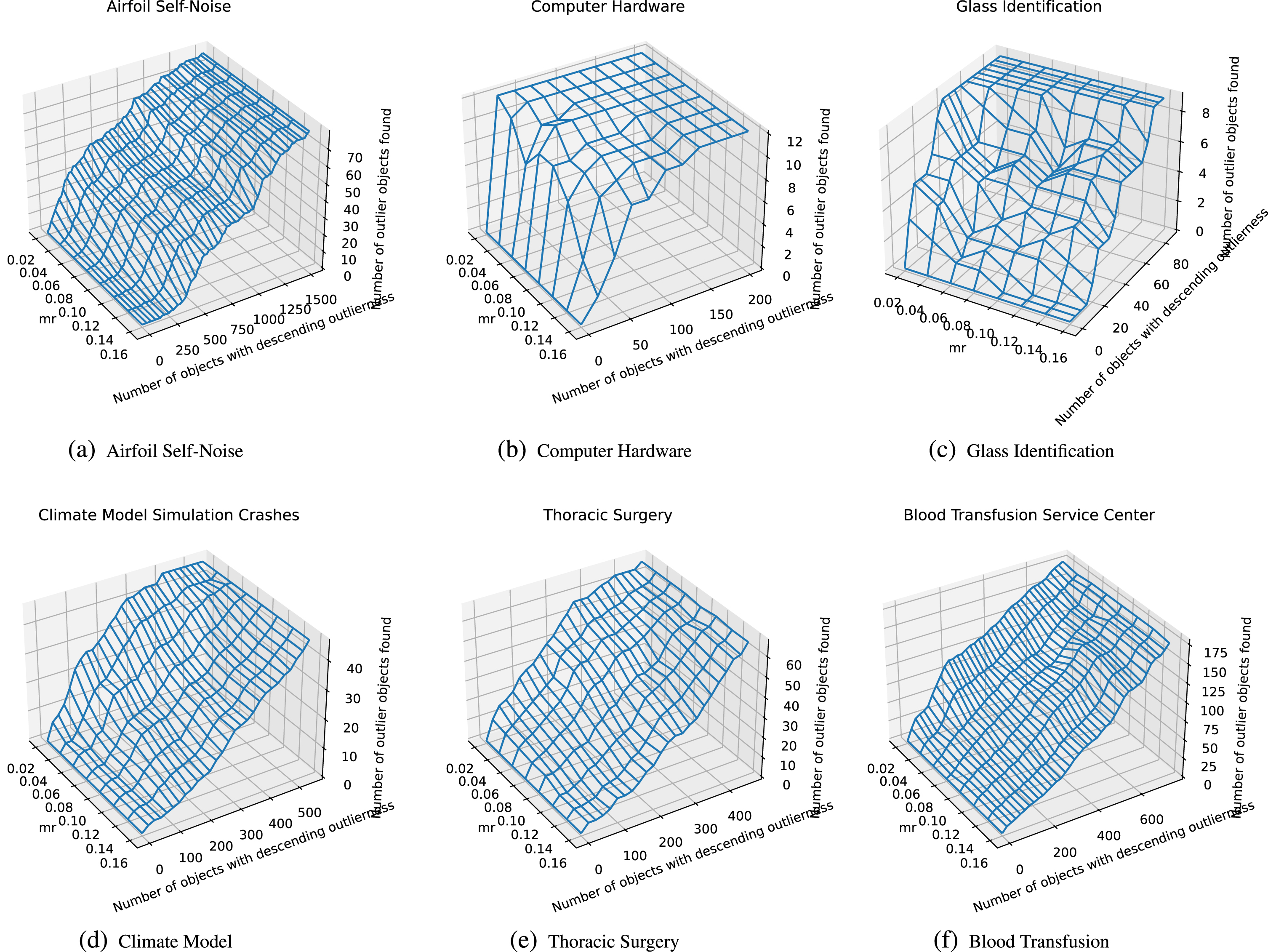
Comparison chart of missing rate analysis.

6 Evaluation analyses

In this section, ROC curve and AUC standard are used to evaluate the experimental results, and Friedman test is performed.

The confusion matrix is required to draw the ROC curve. The confusion matrix is shown in Table 17. There are 4 possible outcomes in the prediction of outliers: an outlier taken as outlier(true positive, TP), an outlier taken as inlier (false negative, FN), an inlier taken as outlier (false positive, FP) and an inlier taken as inlier (true negative, TN).

Table 17
Confusion matrix for predicting an outlier

Predicted outlier Predicted inlier

Actual outlier TP FN

Actual inlier FP TN

	Predicted outlier	Predicted inlier
Actual outlier	TP	FN
Actual inlier	FP	TN

Accordingly, the true positive rate (TPR) and false positive rate (FPR) could be defined as follows:

$TPR = TP / (TP + FN), FPR = FP / (FP + TN)$ (23) After setting a certain threshold, calculate the TPR and FPR corresponding to the threshold, and then draw a corresponding point on the ROC. After setting several thresholds, the ROC curve can be connected. The TPR can also be called “detection rate”, which implies the number of correctly identified outliers, On the contrary FPR displays the original normal instances as outliers. Obviously, when evaluating the performance of the algorithm, these two indicators are often opposite.

AUC is the area under the ROC curve, which means that a positive sample and a negative sample are randomly selected from all samples. The probability of positive sample prediction by the model is P1, and the probability of negative sample prediction is P2. AUC is the probability of P1textgreaterP2 (with higher values being better).

The ROC results in Fig. 5 indicate that the proposed algorithm is stable in all data sets, and its ROC curve is higher to the left compared to other algorithms. A clearer and more powerful conclusion can be drawn from the AUC results table, as shown in Table 18. Each data set in the table corresponds to a bold number that represents the AUC value calculated by the best performing outlier detection algorithm in the current data set. The last row in the table shows the average ranking of all algorithms, and the proposed OF outlier detection algorithm has the highest average ranking, indicating its good detection performance in multiple data sets.

Fig. 5

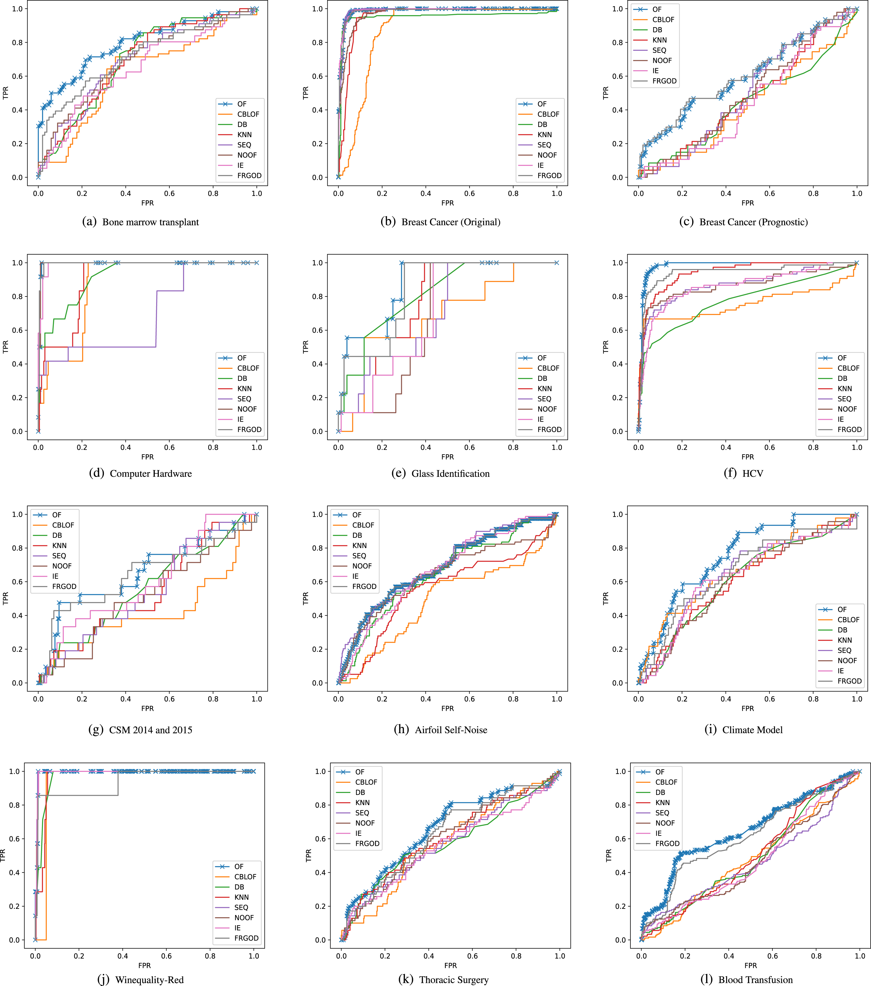
ROC results.

Table 18

AUC results

Data sets	AUC value(rank)
	OF	CBLOF	DB	KNN	SEQ	NOOF	IE	FRGOD
Bone marrow transplant	0.798(1)	0.6213(8)	0.6986(3)	0.695(4)	0.6912(6)	0.6926(5)	0.6467(7)	0.7194(2)
Breast Cancer (Original)	0.9878(3)	0.8754(8)	0.9523(7)	0.9556(6)	0.988(2)	0.971(5)	0.9886(1)	0.9846(4)
Breast Cancer (Prognostic)	0.6019(2)	0.426(8)	0.4406(7)	0.4777(5)	0.5013(3)	0.4913(4)	0.4468(6)	0.6135(1)
Computer Hardware	0.9932(3)	0.8646(7)	0.9181(5)	0.8981(6)	0.6946(8)	0.9949(1)	0.9903(4)	0.9941(2)
Glass Identification	0.8713(1)	0.6813(7)	0.8099(3)	0.7544(4)	0.7047(5)	0.6711(8)	0.7003(6)	0.8363(2)
HCV	0.9808(1)	0.7547(8)	0.7756(7)	0.9421(3)	0.8699(4)	0.8664(5)	0.8615(6)	0.9431(2)
CSM 2014 and 2015	0.6567(1)	0.4181(8)	0.556(4)	0.5449(6)	0.5488(5)	0.5143(7)	0.6016(3)	0.6451(2)
Airfoil Self-Noise	0.6825(3)	0.4899(8)	0.6437(5)	0.5557(7)	0.6938(1)	0.6375(6)	0.6628(4)	0.6853(2)
Climate Model	0.7563(1)	0.6676(2)	0.6083(6)	0.6066(7)	0.6439(4)	0.6065(8)	0.6317(5)	0.6616(3)
Winequality-Red	0.9923(4)	0.9497(7)	0.9723(5)	0.9664(6)	0.994(1)	0.9925(3)	0.993(2)	0.9382(8)
Blood Transfusion	0.6504(1)	0.4785(5)	0.4915(4)	0.503(3)	0.4635(8)	0.4678(7)	0.4753(6)	0.614(2)
Thoracic Surgery	0.6637(1)	0.5755(6)	0.5796(5)	0.6033(3)	0.5721(7)	0.5972(4)	0.5625(8)	0.6291(2)
Average ranking	1.8333	6.8333	5.0833	5	4.5	5.25	4.8333	2.6667

Here we have 8 algorithms and 12 data sets. Considering that each algorithm has a performance ranking on each data set, each algorithm corresponds to a ranking number. The Friedman test and Nemenyi test are also conducted to compare whether there were significant differences between multiple algorithms. Two statistics need to be calculated, namely $X_{F}^{2}$ and F_F. $X_{F}^{2} = \frac{12 N}{k (k + 1)} (\sum_{i = 1}^{k} r_{i}^{2} - \frac{k (k + 1)^{2}}{4}),$ $F_{F} = \frac{(N - 1) X_{F}^{2}}{N (k - 1) - X_{F}^{2}} .$ where N and k represent the number of datasets and algorithms, respectively; $r_{i}^{2}$ indicates the average ranking of a given algorithm across all datasets, and F_F is the F distribution satisfying F (k - 1, (k - 1) (N - 1)) degrees of freedom. If F_F exceeds the critical value F (k - 1, (k - 1) (N - 1)) at significance level α, the original hypothesis is rejected at significance level α. The Nemenyi test can be used to further differentiate algorithm performance. The Nemenyi test adopts the concept of critical difference CD_α, which is defined as follows: ${CD}_{α} = q_{α} \sqrt{\frac{k (k + 1)}{6 N}},$ Where α represents the significance level, and q_α represents the critical value. If the average ranking of two algorithms differs by at least CD_α, then the two algorithms are different at significance level α; Otherwise, it is considered that there is no significant statistical difference between them. According to the final average ranking of each algorithm in Table 18, the Friedman test results are obtained. Taking significance level α=0.1, critical value F (k - 1, (k - 1) (N - 1))=1.796. The calculated F_F of AUC is 7.614, which is greater than critical value.

The comparison of different algorithms with Nemenyi test are shown in Fig. 6. The OF algorithm has the lowest ranking mean under each data set, which is significantly different from the six algorithms with higher ranking.

Fig. 6

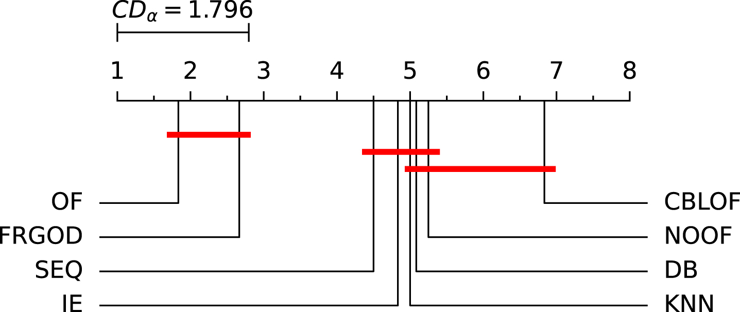
Nemenyi test result.

7 Conclusions

Combining the advantages of RST and GRC, this paper has studied the outlier detection method in an IRVIS. A method for calculating the outlier factor of each object has been constructed. The corresponding outlier detection algorithm has been proposed. Several experiments on twelve data sets have been carried out. When the performance of the other six algorithms fluctuates with different data sets, the proposed algorithm remains relatively stable and has certain robustness. This shows that the performance of the proposed algorithm is better than the other six algorithms. In future work, we will consider optimizing the proposed algorithm to reduce the computational time while the performance of the algorithm is maintained, and study outlier detection for hybrid data.

Footnotes

Acknowledgments

The authors would like to thank the editors and the anonymous reviewers for their valuable comments and suggestions, which have helped immensely in improving the quality of the paper. This work is supported by Guangxi First-class Discipline Statistics Construction Project Fund and Natural Science Foundation of Guangxi Province (2021GXNSFAA220114).

References

Al-Shami

T.M.

, Maximal rough neighborhoods with a medical application, Journal of Ambient Intelligence and Humanized Computing 2022. https://link.springer.com/article/10.1007/s12652-022-03858-1

Al-Shami

T.M.

, An improvement of rough setsaŕ accuracy measure using containment neighborhoods with a medical application, Information Sciences 569 (2021), 110–124.

Al-Shami

T.M.

, Topological approach to generate new rough set models, Complex & Intelligent Systems 8 (2022), 4101–4113.

Al-Shami

T.M.

, Improvement of the approximations and accuracy measure of a rough set using somewhere dense sets, Soft Computing 25 (2021), 14449–14460.

Al-Shami

T.M.

and Alshammari

, Rough sets models inspired by supra-topology structures, Artificial Intelligence Review 2022. https://link.springer.com/article/10.1007/s10462-022-10346-7

Al-Shami

T.M.

and Ciucci

, Subset neighborhood rough sets, Knowledge-Based Systems 237 (2022), 107868.

Al-Shami

T.M.

and Hosny

, Improvement of approximation spaces using maximal left neighborhoods and ideals, IEEE Access 10 (2022), 79379–79393.

Al-Shami

T.M.

and Mhemdi

, Approximation operators and accuracy measures of rough sets from an infra-topology view, Soft Computing 27 (2023), 1317–1330.

Aggarwal

C.C.

and Philip

S.Y.

, An effective and efficient algorithm for high-dimensional outlier detection, VLDB J 14(2) (2005), 211–221.

10.

Aggarwal

C.C.

and Yu

P.S.

, Outlier detection for high dimensional data, in: Proceedings of the 2001 ACM SIGMOD international conference on Management of data, 2001; 37–46.

11.

Breunig

M.M.

, Kriegel

H.P.

, Ng

R.T.

, et al., LOF: identifying density-based local outliers, in: Proceedings of the 2000 ACMSIGMOD international conference on Management of data, 2000; 93–104.

12.

Barnett

and Lewis

, Outliers in statistical data, John Wiley and Sons, New York, 1994.

13.

Chandola

, Banerjee

and Kumar

, Outlier detection: A survey, ACM Computing Surveys 41(3) (2009).

14.

Chen

H.M.

, Li

T.R.

, Da

, Lin

J.H.

and Hu

C.X.

, A rough-set-based incremental approach for updating approximations under dynamic maintenance environments, IEEE Transactions on Knowledge and Data Engineering 25(2) (2013), 274–284.

15.

Chen

Y.M.

, Miao

D.Q.

and Zhang

H.Y.

, Neighborhood outlier detection, Expert Systems with Applications 37(12) (2010), 8745–8749.

16.

Domingues

, Filippone

, Michiardi

, et al., A comparative evaluation of outlier detection algorithms: Experiments and analyses, Pattern Recognition 74 (2018), 406–421.

17.

Dai

J.H.

, Hu

Q.H.

, Zhang

J.H.

, Hu

and Zheng

N.G.

, Attribute selection for partially labeled categorical data by rough set approach, IEEE Transactions on Cybernetics 47(9) (2017), 2460–2471.

18.

Dey

, Kumar

B.R.

, Das

and Ghoshal

A.K.

, Outlier detection in social networks leveraging community structure, Information Sciences 634 (2023), 578–586.

19.

Francisco

M.P.

, Josĺe

V.B.M.

, Alberto

F.O.

and Miguel

A.O.

, Algorithm for the detection of outliers based on the theory of rough sets, Decision Support Systems 75(C) (2015), 63–75.

20.

Gao

, Cai

M.J.

and Li

Q.G.

, A relative granular ratio-based outlier detection method in heterogeneous data, Information Sciences 622 (2023), 710–731.

21.

Hawkins

D.M.

, Identification of outliers, Chapman and Hall, London, 1980.

22.

Hosny

, Al-Shami

T.M.

and Mhemdi

, Novel approaches of generalized rough approximation spaces inspired by maximal neighbourhoods and ideals, Alexandria Engineering Journal 69 (2023), 497–520.

23.

Hawkins

, He

, Williams

G.J.

and Baxter

R.A.

, Outlier detection using replicator neural networks. CiteSeer, International Conference on Data Warehousing and Knowledge Discovery, Springer, Berlin, Heidelberg (2002), 170–180.

24.

, Xu

and Deng

, Discovering cluster-based local outliers, Pattern Recognition Letters 24(9-10) (2003), 1641–1650.

25.

Jain

A.K.

, Murty

M.N.

and Flynn

P.J.

, Data clustering: a review, ACM Computing Surveys 31(3) (1999), 264–323.

26.

Jiang

and Chen

Y.M.

, Outlier detection based on granular computing, International Conference on Rough Sets and Current Trends in Computing Springer-Verlag, 2008.

27.

Jiang

, Sui

Y.F.

and Cao

C.G.

, An information entropy-based approach to outlier detection in rough sets, Expert Systems with Applications 37(9) (2010), 6338–6344.

28.

Jiang

, Sui

Y.F.

and Cao

C.G.

, Some issues about outlier detection in rough set theory, Expert Systems with Applications 36 (2009), 4680–4687.

29.

Jiang

, Zhao

H.B.

, Du

J.W.

, Xue

and Peng

Y.J.

, Outlier detection based on approximation accuracy entropy, International Journal of Machine Learning and Cybernetics 10(9) (2018), 2483–2499.

30.

Knorr

E.M.

, Ng

R.T.

and Tucakov

, Distance-based outliers: algorithms and applications, The VLDB Journal 8(3) (2000), 237–253.

31.

Lan

, et al., A survey of data mining and deep learning in bioinformatics, Journal of Medical Systems 42(8) (2018), 139.

32.

Lin

T.Y.

, Data Mining and Machine Oriented Modeling: A Granular Computing Approach, Applied Intelligence 13(2) (2000), 113–124.

33.

Liu

, Yu

, Song

, et al., Scalable KDE-based top-n local outlier detection over large-scale data streams, Knowledge-Based Systems 204(9) (2020), 106186.

34.

Miao

D.Q.

, Wang

G.Y.

, Liu

, Lin

T.Y.

and Yao

Y.Y.

, Granular computing: past, present and future prospect, Science Press, Beijing, 2007.

35.

Mustafaa

H.I.

, Al-Shami

T.M.

and Wassefa

, Rough set paradigms via containment neighborhoods and ideals, Filomat 37 (2023), 4683–4702.

36.

Macia-Perez

, Berna-Martinez

J.V.

, Oliva

A.F.

and Ortega

M.A.A.

, Algorithm for the detection of outliers based on the theory of rough sets, Decision Support System 75 (2015), 63–75.

37.

Pal

S.K.

, Meher

S.K.

and Dutta

, Class-dependent rough-fuzzy granular space, dispersion index and classification, Pattern Recognition 45(7) (2012), 2690–2707.

38.

Papadimitriou

, Kitagawa

, Gibbons

P.B.

and Faloutsos

, LOCI: Fast outlier detection using the local correlation integral, in: Proceedings of IEEE International Conference on Data engineering, 2003, pp. 315–326.

39.

Pawlak

, Rough sets, International Journal of Computer and Information Science 11 (1982), 341–356.

40.

Pawlak

, Rough Sets: Theoretical Aspects of Reasoning about Data, Kluwer Academic Publishers, Dordrecht, 1991.

41.

Rousseeuw

P.J.

and Leroy

A.M.

, Robust regression and outlier detection, Journal of the American Statistical Association 31(2) (1987), 260–261.

42.

Ramaswamy

, Rastogi

and Shim

, Efficient algorithms for mining outliers from large data sets, in: Proceedings of the 2000 ACM Sigmod international conference on Management of data, 2000, pp. 427–438.

43.

Wang

C.Z.

, Huang

, Shao

M.W.

, Hu

Q.H.

and Chen

D.G.

, Feature selection based on neighborhood self-information, IEEE Transactions on Cybernetics 50(9) (2020), 4031–4042.

44.

Yao

Y.Y.

, Granular computing using neighborhood systems, in: Advances in Soft Computing: Engineering Design and Manufacturing, 1999, pp. 539–553.

45.

Yao

Y.Y.

, Granular computing for data mining, in: Proceedings of SPIE conference on data mining, intrusion detection, information assurance, and data networks security, 2006, pp. 1–12.

46.

Yuan

, Chen

H.M

, Li

T.R.

, Liu

and Wang

, Fuzzy information entropy-based adaptive approach for hybrid feature outlier detection, Fuzzy Sets and Systems 421 (2021), 1–28.

47.

Yuan

, Chen

, Li

, et al., Outlier detection based on fuzzy rough granules in mixed attribute data, IEEE Transactions on Cybernetics 52(8) (2021), 8399–8412.

48.

Yao

J.T.

, Vasilakos

A.V.

and Pedrycz

, Granular computing: Perspectives and challenges, IEEE Transactions on Cybernetics 43 (2013), 1977–1989.

49.

Zadeh

L.A.

, Towards a theory of fuzzy information granulation and its centrality in human reasoning and fuzzy logic, Fuzzy Sets and Systems 90(2) (1997), 111–127.

50.

Zhao

S.Y.

, Chen

, Li

C.P.

, Du

X.Y.

and Sun

, A novel approach to building a robust fuzzy rough classifier, IEEE Transactions on Fuzzy System 23 (2015), 769–786.

51.

Zhang

Q.H.

, Yang

S.H.

and Wang

G.Y.

, Measuring uncertainty of probabilistic rough set model from its three regions, IEEE Transactions on Systems, Man and Cybernetics (Part A) 47 (2017), 3299–3309.

Outlier detection for incomplete real-valued data via rough set theory and granular computing

Abstract

Keywords

1 Introduction

1.1 The relevant research work

1.2 Motivation and contributions

2.2 An IRVIS

5.1 Experimental setup

5.2 Data sets

Table 17 Confusion matrix for predicting an outlier Predicted outlier Predicted inlier Actual outlier TP FN Actual inlier FP TN

Footnotes

Acknowledgments

References

Table 17
Confusion matrix for predicting an outlier

Predicted outlier Predicted inlier

Actual outlier TP FN

Actual inlier FP TN