An adaptive indoor localization model based on Cauchy-PSO optimized BPNN

Abstract

Received Signal Strength Indication (RSSI) fluctuates with the change of indoor noise, resulting in a large positioning error of the trained Back Propagation Neural Network (BPNN). An adaptive indoor positioning model based on Cauchy particle swarm optimization (Cauchy-PSO) BPNN is proposed to solve the problem. In the off-line training phase, the signal with less noise intensity acquired in a good environment is selected as the original training set in the localization phase. The variance of the received set of signals is used as a measure of the noise intensity of the current environment. In the localization phase, the variance of each set of signals received is calculated at equal intervals. If the variance of adjacent intervals differs significantly, the system adjusts the original training set data according to the current noise intensity and re-trains the BP model online. Meanwhile, the particle swarm optimization algorithm using Cauchy variance to optimize the BP network tends to fall into the disadvantage of local optimum. Considering that the collected fingerprint database may generate “high-dimensional disasters”, Principal Component Analysis (PCA) is used to select and downscale the features of the wireless Access Point (AP). The proposed adaptive localization model can be trained online. The improved Cauchy-PSO algorithm and data dimensionality reduction can further improve the localization accuracy and training speed of the BP model. The experimental results show that the adaptive indoor localization model has strong adaptive capability in a noise-varying environment.

Keywords

RSSI adaptive BP model (AI-BP)BPNN PCA Cauchy-PSO

1 Introduction

With the increasing demand for indoor positioning services, a variety of positioning techniques have been applied in the fifield of indoor positioning. Among them, location fifingerprint-based matching techniques such as cellular signals and Wi-Fi signals have become the focus of research on indoor positioning due to their advantages of high positioning accuracy, high feasibility, low cost, and no additional hardware investment [1 –6]. In recent years, a variety of positioning algorithms have been proposed [7 –10]. There are also many examples of combining neural networks with RSSI [11 –15], among which, the BPNN-based RSSI localization approach is widely used [16 –18]. However, the traditional BPNN-based localization algorithm has limited adaptability. Due to the complexity of the indoor environment and the randomness of people, the RSSI will be affected by noise, resulting in a large positioning error of the trained BPNN [19 –21]. Besides, the BPNN localization model has some shortcomings, such as slow convergence speed and easy falling into local optimum, for which several scholars have proposed improvements to the relevant localization algorithms.

A method combining the annealing algorithm with the genetic algorithm is proposed in [22] to optimize the neural network and apply it to an indoor location. Compared with the traditional model based on the BPNN, the positioning accuracy of RSSI is improved by about 60%. In [23], the PSO-BP algorithm is proposed, which is used to optimize the shortcomings of BPNN and improve the indoor positioning accuracy. A new ranging model is proposed in [24], using a genetic algorithm to optimize the initial values of weights and deviations of the BPNN, which improves the positioning accuracy of this model. In [25], the advantages of genetic algorithm and particle swarm optimization algorithm are expounded and combined to make up for the shortcomings of the traditional BPNN algorithm. These studies have made innovations in BPNN and RSSI positioning, and provided many improvement directions, but they did not consider the changing factors of indoor environment.

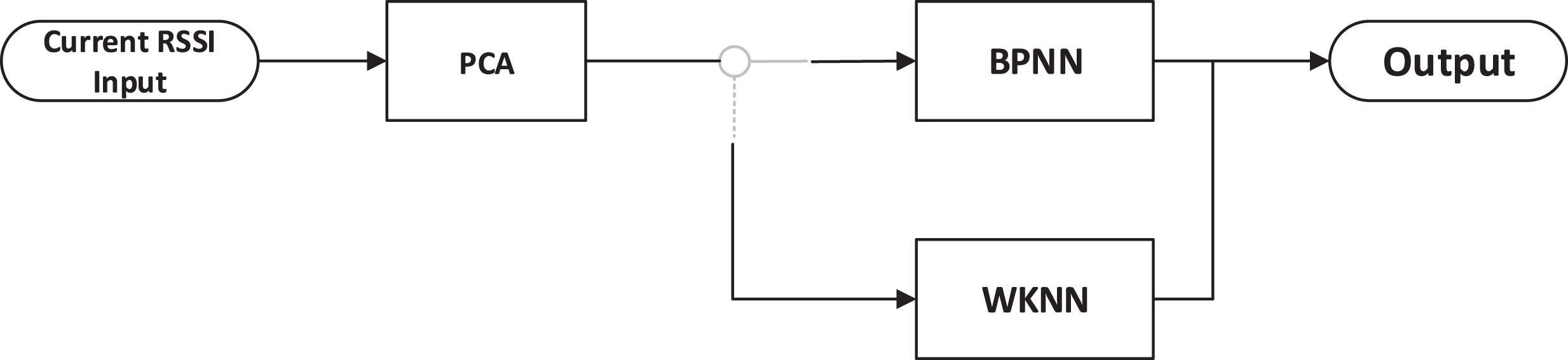
In this paper, an adaptive indoor positioning structure based on Cauchy-PSO improved BPNN is proposed. This algorithm can make up for the influence of environmental changes in indoor positioning. First, we use PCA to reduce the dimensionality of the collected fingerprint database to improve the training speed of the BPNN. Then an adaptive BP model is constructed. The BPNN under this model can be changed according to the change of environment, which ensures that the current BPNN can adapt to the current environment. Finally, the shortcomings of BPNN are optimized by Cauchy-PSO algorithm. The overall architecture diagram is shown in Fig. 1.

Fig. 1

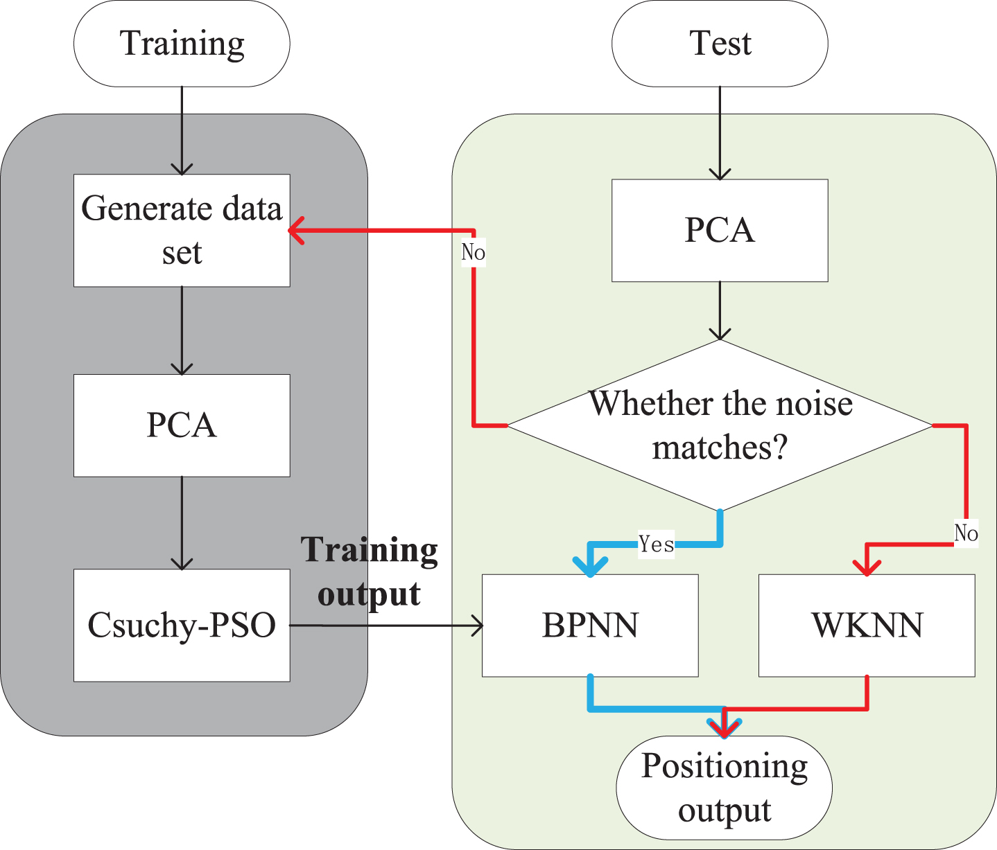
The overall architecture diagram.

The structure of this paper is as follows: Section 2 introduces the PCA dimension reduction algorithm. Section 3 introduces the adaptive BP model. Section 4 introduces the Cauchy-PSO algorithm and the Cauchy-PSO-BP positioning model. Section 5 describes the experiment and discusses the results obtained, and section 6 summarizes the paper.

2 Dimension reduction algorithm of principal component analysis

PCA is a data dimensionality reduction algorithm, which can reduce the dimensionality of high-dimensional data to a lower dimension on the premise of retaining the original data features [26 –28]. The PCA algorithm can maintain the uniformity of data dimensionality. Although the data contains less information after dimensionality reduction, the dimensionality reduction is more beneficial to the system and speeds up the processing of data. PCA is used to reduce the dimension of (x (1) , x (1) , …, x (m)) with m n-dimensional data sets. $x (i) = x (i) - \frac{1}{m} \sum_{j = 1}^{m} x (j) .$ (1) The algorithm flow of dimension reduction is as follows:

Step 1: Use (1) to center each sample feature.

Step 2: Calculating the covariance matrix of the sample and decompose the eigenvalue.

Step 3: Extracting the eigenvectors corresponding to the largest eigenvalues, then all the feature vectors are standardized to form the feature vector.

Step 4: Calculate the new sample after dimension reduction and obtain the dimensionality reduction result.

3 Adaptive BP localization model

3.1 BP neural network (BPNN) model

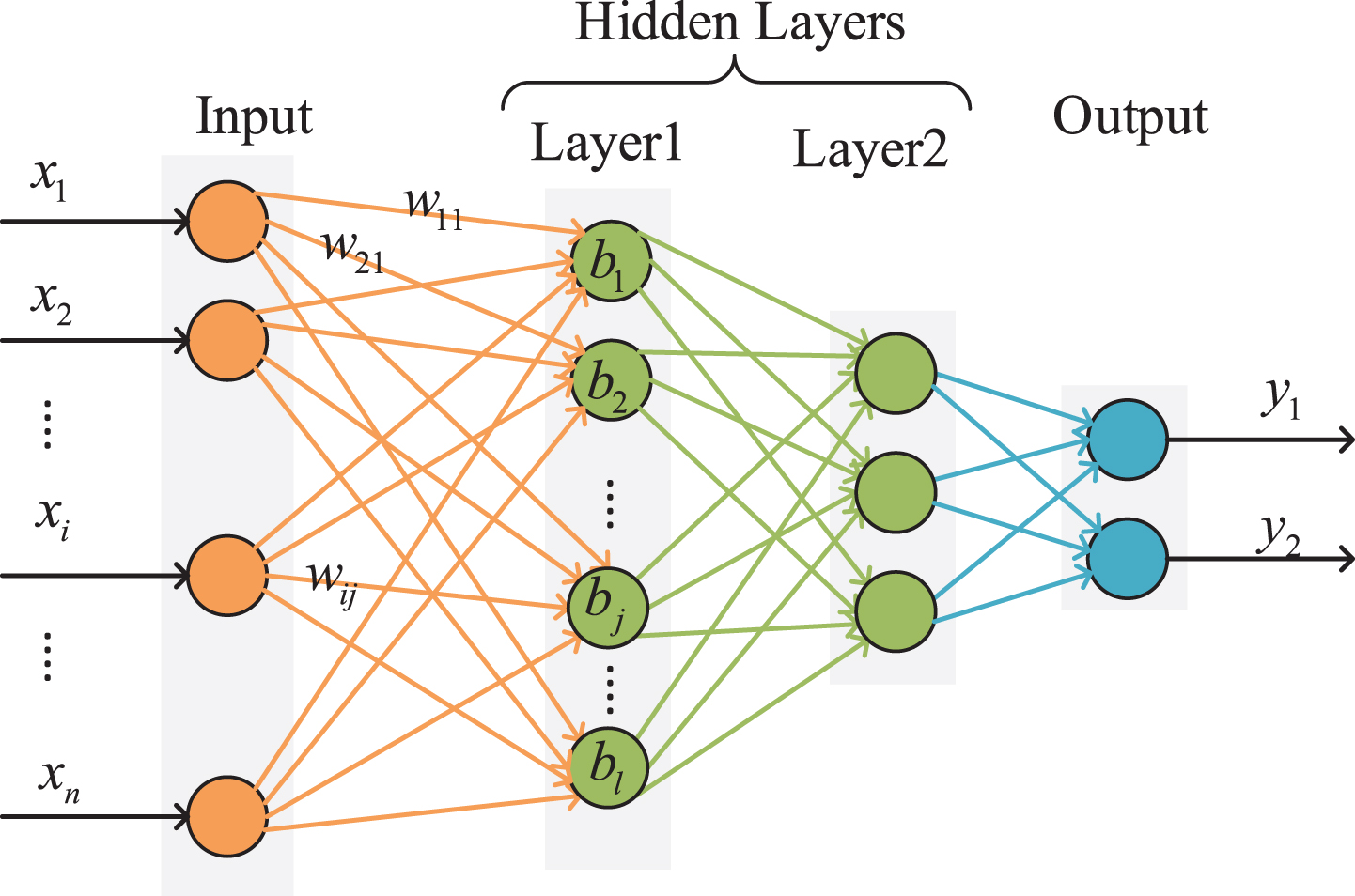
BPNN is a multi-layer feedforward neural network. The basic idea of its algorithm consists of forward propagation of signal and backward propagation of error. The error is minimized by constantly changing the weight and threshold of BPNN. Forward propagation is the propagation process of signals from the input layer through the hidden layer and finally to the output layer, while reverse propagation is the opposite. In this propagation process, the initial weights and thresholds of each layer of the neural network are constantly adjusted, so as to achieve the purpose of training the neural network [29]. Figure 2 shows the schematic diagram of the double hidden layer BP. In order to express the process of back propagation conveniently, a cost function (2) is defined.

Fig. 2

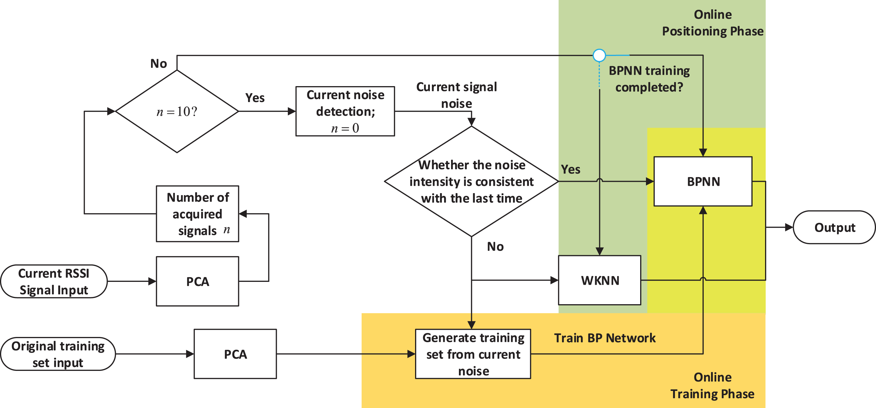
Adaptive positioning model.

$C (w, b) \equiv \frac{1}{2 n} \sum_{x} ∥ y (x) - a ∥^{2},$ (2) where, $y (x) = [\begin{matrix} y_{1} \\ y_{2} \end{matrix}]$ represents the output of BPNN when the input is x, a represents the actual output vector when the input is x, and n is the number of training sets of BPNN. Equation (3) is the update rule of weight and bias. $w_{ji} = w_{ji} - η \frac{\partial C}{\partial w_{ji}}, b_{j} = b_{j} - η \frac{\partial C}{\partial b_{j}},$ (3) where, η represents the learning rate, w_ji represents the weight between the i-th neuron in the previous layer and the j-th neuron in the next layer, and b_j represents the bias of the j-th neuron.

3.2 Adaptive BP model construction

The acquired signal is reduced in dimension by PCA and stored in the memory. If the signal value is not collected for 10 times, the BPNN is used for positioning. After collecting the signal values for 10 times, the memory starts to calculate the variance of the current signal. The larger the variance, the more serious the noise in the current environment. This process is called environmental noise intensity detection. If the variance of the current signal is quite different from that of the BP training set signal, it means that the BP model after the last training is no longer suitable for the current environment. Therefore, it is necessary to readjust the BP training set data to make it fit the current environment, then retrain the BP model. Weighted K-Nearest Neighbor (WKNN) is used for positioning temporarily in the process of BPNN training and the positioning of BPNN is resumed after the training of the model. At this time, the trained BPNN is more suitable for the current environment. Figure 3 shows the adaptive positioning model based on BPNN.

Fig. 3

BP double hidden layer feedforward network.

Off-line training stage: Each positioning point repeatedly collects multiple sets of data when the environmental (e.g., at night) noise is low. The average value is calculated and used as the original training set of BP model. Figure 4 is the flow chart of offline training stage.

Fig. 4

Off-line training phase.

On-line training stage: After noise detection, the original training set data will be added with corresponding Gaussian noise if the BPNN needs to be retrained. The purpose of this step is to make the noise intensity of the training set match that of the current signal, and then the training data set will be used to train the BPNN. In the training stage, WKNN is used for positioning. Figure 5 is the flow chart of online training stage.

Fig. 5

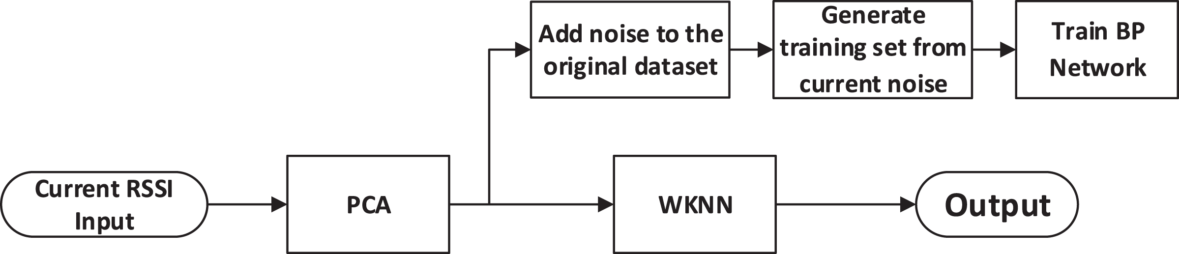
On-line training phase.

If the BP model does not need to be retrained after noise detection, or the RSSI values are not collected for 10 times in the memory, then the BPNN is directly used for positioning; if the BPNN needs to be retrained, the WKNN is used for positioning. Figure 6 is the flow chart of online positioning stage.

Fig. 6

On-line positioning stage.

4 Cauchy-PSO optimization BPNN positioning algorithm

4.1 Cauchy-PSO algorithm

In the traditional particle swarm optimization algorithm, some particles are initially generated. X_i = (x_i1, x_i2, ⋯ , x_iD) is the position vector of particle i, V_i = (v_i1, v_i2, ⋯ , v_iD) represents the velocity vector of particle i, where D represents the dimension of particle space. The algorithm gets the optimal solution through repeated iterations, and each iteration updates the values of Pbest and Gbest [30, 31]. Pbest is the historical optimal position of particle i, Gbest is the optimal position of the whole group. The particle position matrix and velocity matrix are updated by the following formula: $\begin{matrix} V_{iD}^{k - 1} = {wV}_{iD}^{k} & + c_{1} \times rand \times (P_{best iD}^{k} - x_{iD}^{k}) \\ + c_{2} \times rand \times (G_{best iD}^{k} - x_{iD}^{k}), \end{matrix}$ (4) $x_{iD}^{k + 1} = x_{iD}^{k} + V_{iD}^{k + 1} .$ (5) Where, i = 1, 2, ⋯ , N, N is the sum of the number of particles in the particle group; V_i is the velocity of the particle; rand is a random number between 0-1; X_i is the current position of the particle; c₁, c₂ is a learning factor with a value of 1.5; w is the inertia weight factor. Traditional PSO algorithm may still be premature and fall into local optimum. To alleviate this problem, Cauchy mutation is introduced, which can not only keep the diversity δ of particle swarm, but also make the optimization algorithm avoid local optimum [32]. When the aggregation degree of particle swarm is less than Cauchy mutation probability, the position of particle swarm is disturbed. f (x_i) represents the fitness value of the i-th particle, f_avg represents the average fitness value of the particle swarm [33]. The aggregation degree δ is defined as follows: $δ = \frac{1}{N} \sum_{i = 1}^{N} {| \frac{f (x_{i}) - f_{avg}}{h} |}^{2},$ (6) where h is the control factor. h is defined as follows:

$h = max {1, max | f (x_{i}) - f_{avg} |} .$ (7)

In this paper, Cauchy mutation probability is set to 0.5. When δ < 0.5, Cauchy mutation is introduced to disturb the position of particle swarm. Equation (8) is the calculation method of Cauchy operator. $Cauchy = tan ((rand - \frac{1}{2}) \times π) .$ (8)

Equation (9) is the way Cauchy variation disturbs the particle position. $x_{i} = x_{i} \times (1 + 0.3 \times Cauchy) .$ (9) The algorithm steps are as follows:

Step 1: Initializing particle swarm parameters to generate particle swarm.

Step 2: Calculate the particle fitness, and determine the individual optimal P_best and the global optimal G_best.

Step 3: Update the position matrix and speed matrix.

Step 4: Calculate the aggregation degree of particle swarm and judge whether Cauchy variation exists.

Step 5: Judging whether the algorithm meets the loop end condition, if so, executing step 6, otherwise, returning to step 2 and continuing to execute step 2 to step 5.

Step 6: Outputting the global optimal G_best and particle position vector, and ending the algorithm.

4.2 Cauchy-PSO improved BPNN model algorithm (Cauchy-PSO-BP)

Firstly, the initial weights and thresholds of BPNN are normalized. Then the Cauchy-PSO algorithm is applied to iteratively optimize the position of the optimal particle. The optimal particle position is used as the initial weight and bias of the training BPNN. Finally, the training model is output and applied to RSSI positioning. Figure 7 is the flowchart of Cauchy-PSO-BPNN algorithm.

Fig. 7

Flow chart of Cauchy-PSO-BP network model.

4.3 Algorithm description and pseudo-code

The whole algorithm flow includes generating dataset, training the BPNN model, and testing the positioning output.

Generating dataset: Generating a set of original data sets when noise intensity is low, and removing “high-dimensional redundancy” through PCA dimension reduction.

Training BPNN model: Use RSSI value after PCA dimension reduction as training set to train BPNN model.

Test positioning output: Calculate the current noise intensity. If it does not match the noise intensity in the training stage, retrain the BPNN model and use WKNN for temporary localization.

Algorithm 1 Generate Dataset
Input: RSSI value, noise intensity P_BPnoise, raw dataset D;
Output: Dataset D_noise at noise intensity P_noise
1. Use D and P_noise to generate a dataset under
the current noise intensity;
2. Delete invalid data;
3. PAC dimensionality reduction;
4. Output Dataset D_noise;

Algorithm 2 Training BPNN Model
Input: Training Set D_noise, Noise Intensity P_BPnoise;
Output: BPNN model, noise intensity P_BPnoise;
1. Using Algorithm 1 to generate a dataset as a training set;
2. Training BPNN;
3. Output BPNN model;

Algorithm 3 Positioning output
Input: RSSI value, BPNN model output using algorithm 2,
and noise intensity P_BPnoise;
Output: Positioning output
1. Calculate the current noise intensity P_noise;
2. if P_noise and P_BPnoise matching
Use BPNN positioning to output positioning results;
else
Use WKNN positioning to output positioning results.
Retraining BPNN using Algorithm 2.
End

5 Experiment results and analysis

In this paper, the performance of the positioning algorithm is tested and verified by virtual simulation. The data set is generated according to the logarithmic path loss model (10). In (10), P_r (d) and P_r (d₀) respectively represent the received power at the distance between the test point and the wireless access point of d and d₀. n is the path attenuation factor, which is related to the specific environment. X is a Gaussian random variable with an average value of 0.

P_{r} (d) = P_{r} (d_{0}) + 10 n lg (\frac{d}{d_{0}}) + X .

(10)

Usually, d₀ is 1m, P_r (d₀)is the received signal strength value of the receiving node 1m away from the transmitting node. The propagation model can be simplified as (11) [34]:

RSSI = A - 10 n lg (d) + X .

(11)

In this experiment, A = -41.3dB, n = 1.58, according to the above loss model, firstly, a 10 m × 10 m virtual environment is generated by MATLAB. The distance between adjacent receiving points is 1 m, the layout of beacon nodes is arc triangle layout model [35], and the distance between adjacent beacon nodes is 5 m. The area surrounded by three arcs is arc triangle. The layout of beacon nodes is shown in Fig. 8. A total of 149 location points are selected by removing the beacon nodes on the location points.

Fig. 8

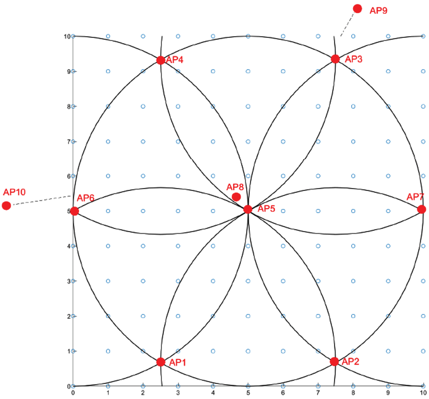
Schematic diagram of AP location.

5.1 Performance of PCA algorithm

In Fig. 8, AP5 and AP8 are adjacent to each other, so they contain similar features. The power of the signal to the receiving point is very weak because AP9 and AP10 is far from the positioning point. The existence of AP5, AP9 and AP10 causes the redundancy of fingerprint database. Therefore, PCA is used to reduce the dimension of fingerprint database.

5.1.1 PCA experiment preparation

Firstly, in a virtual model with 10 APs, each location point is sampled 100 times repeatedly. Gaussian random noise is added to the sampled RSSI values, the first 80 times as the training set and the last 20 times as the test set.

5.1.2 Impact of fingerprint database degradation on localization

The influences include: the energy ratio of different AP numbers, the training speed of BPNN and the positioning error. The reduced fingerprint database is used as the training set of BPNN. Figure 9 shows the positioning error based on BPNN under different numbers of access points. It can be seen from Fig. 9 that the positioning accuracy increases slightly when beacon nodes are added. The ratio of energy contained in different AP numbers and the training time required when BPNN training times are 1000 are shown in Table 1. According to the ratio of energy in Table 1, seven APs already contain 99.89% of the total energy, which shows that AP8, AP9 and AP10 hardly play any role in the positioning process and they also cause the redundancy of fingerprint database. In terms of training time, dimensionality reduction of fingerprint database can improve the training speed of BPNN. From the aspect of positioning error, adding AP is equivalent to increasing the characteristic information of fingerprint database, which can reduce the positioning error. However, the experimental results show that the added AP information is mostly redundant information, which has little effect on positioning and increases the training time of BPNN. Considering that the AP signal with extremely long distance is very unstable in the real environment, and at the same time, the intermittent signal will also cause uneven dimension and dimension disaster in the fingerprint database, so the following experiments all use AP1–AP7 as the positioning signal source.

Fig. 9

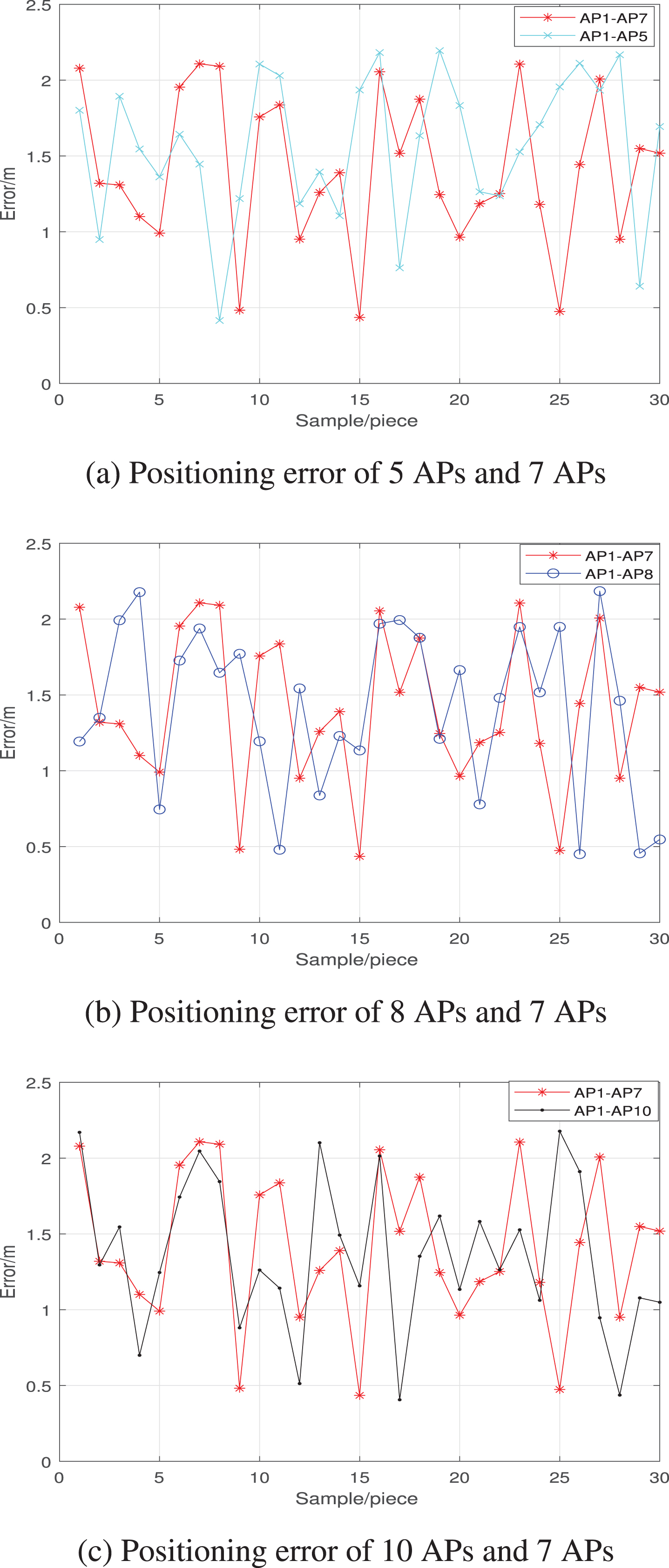
Positioning error of different number of APs.

Table 1

Effect of different numbers of AP on positioning

Ap Number	Energy ratio	BP training time	Average error
AP1-AP10	100%	15.1613s	1.3645m
AP1-AP8	99.99%	13.8475s	1.4149m
AP1-AP7	99.89%	11.2679s	1.4262m
AP1-AP5	98.71%	10.0136s	1.5625m

5.2 Performance of adaptive BP model

5.2.1 BP model initialization

After PCA dimensionality reduction, AP1-AP7 are used as positioning signal sources, so the number of input layer nodes of BPNN is seven. The positioning results are output in the form of coordinates, so the number of output layer nodes of BPNN is 2. The number of hidden layer nodes directly affects the positioning effect of BPNN. Through many positioning tests and analysis, the positioning effect is the best when the number of hidden layer nodes is 13. Based on the above analysis, the number of nodes in the input layer, hidden layer and output layer of BPNN is determined to be 7, 13 and 2, respectively. The training times are 1000 times, the learning rate is set to 0.1, the training target error is 10^-5, and the activation functions of the hidden layer and the output layer are tansig and purelin functions respectively.

5.2.2 Localization error of adaptive BP model and other models

Considering personnel activities and other factors, the noise power intensity will be different in different time periods in a day. According to the difference of personnel flow in each time period, a day is divided into four time periods, which are 6:00–8:00, 8:00–18:00, 18:00–22:00, and 22:00–6:00 the next day, respectively. Figure 10 shows the RSSI value of AP1 received by a certain positioning point in a day. As can be seen from Fig. 10, the fluctuation of the received signal power value is the smallest from 22:00 to 6:00 the next day, and the largest from 8:00 to 18:00.

Fig. 10

RSSI values at different moments.

According to the above environment, the positioning errors based on BP, PSO-BP and adaptive BP models are compared. In the off-line phase, select the signal with noise intensity in the period of 6:00–8:00 as the training set. In the on-line phase, the signals of different time periods in a day are selected as test sets. After the model training is completed, the three models are predicted and positioned respectively.

Figure 11 shows the positioning errors when 6:00–8:00, 8:00–18:00, 18:00–22:00 and 22:00–6:00 are taken as test sets, where AI-BP is an adaptive positioning model. When the noise intensity changes little, the PSO-BP positioning algorithm has high positioning accuracy. However, after the noise intensity changes, the AI-BP positioning algorithm has higher positioning accuracy than the BP and PSO-BP positioning algorithms. Table 2 shows the positioning errors of the three algorithms over different time periods.When the noise changes, compared with the traditional BP algorithm and PSO-BP algorithm, the adaptive BP algorithm has higher positioning accuracy and is more suitable for the noise changing environment. At the same time, because the BP model itself easily falls into the local optimum, it is necessary to optimize the BP algorithm by PSO.

Fig. 11

Localization errors of BP, PSO-BP and AI-BP at different time periods.

Table 2

Comparison of location average errors under different time periods

Algorithm	6:00–8:00	8:00–18:00	18:00–22:00	22:00–6:00
BP	0.745m	1.630m	1.362m	0.648m
PSO-BP	0.612m	1.025m	1.224m	0.538m
AI-BP	0.757m	1.309m	1.058m	0.441m

5.3 Cauchy-PSO optimizes the performance of BPNN

Cauchy-PSO algorithm is introduced to optimize BPNN, which mainly solves the problems of slow convergence speed, many iterative steps, and easy to fall into local optimal solution.

5.3.1 Cauchy-PSO algorithm initialization

According to the BPNN topological structure diagram, it is determined that the dimension of particles is 132, the population number of particles is 20, c ₁, c₂ the learning factors are all 1.494, w is set as the nonlinear inertia weight, and the speed and position of each particle are between -1–1.

5.3.2 Location accuracy of Csuchy-PSO algorithm

At first, 20 real positioning points are randomly generated and the generated positioning points may coincide. Then, signals from 18:00 to 22:00 are taken as prediction inputs. Finally, PSO-BP, SA-GA-BP and Csuchy-PSO-BP algorithms are used to predict. The deviation between the predicted point and the real positioning point is shown in Fig. 12, where the red diamond indicates the real position. Figure 13 is an error comparison of three positioning algorithms. Table 3 shows that compared with PSO-BP and SA-GA-BP, the improved BP model of Csuchy-PSO algorithm has smaller positioning errors.

Fig. 12

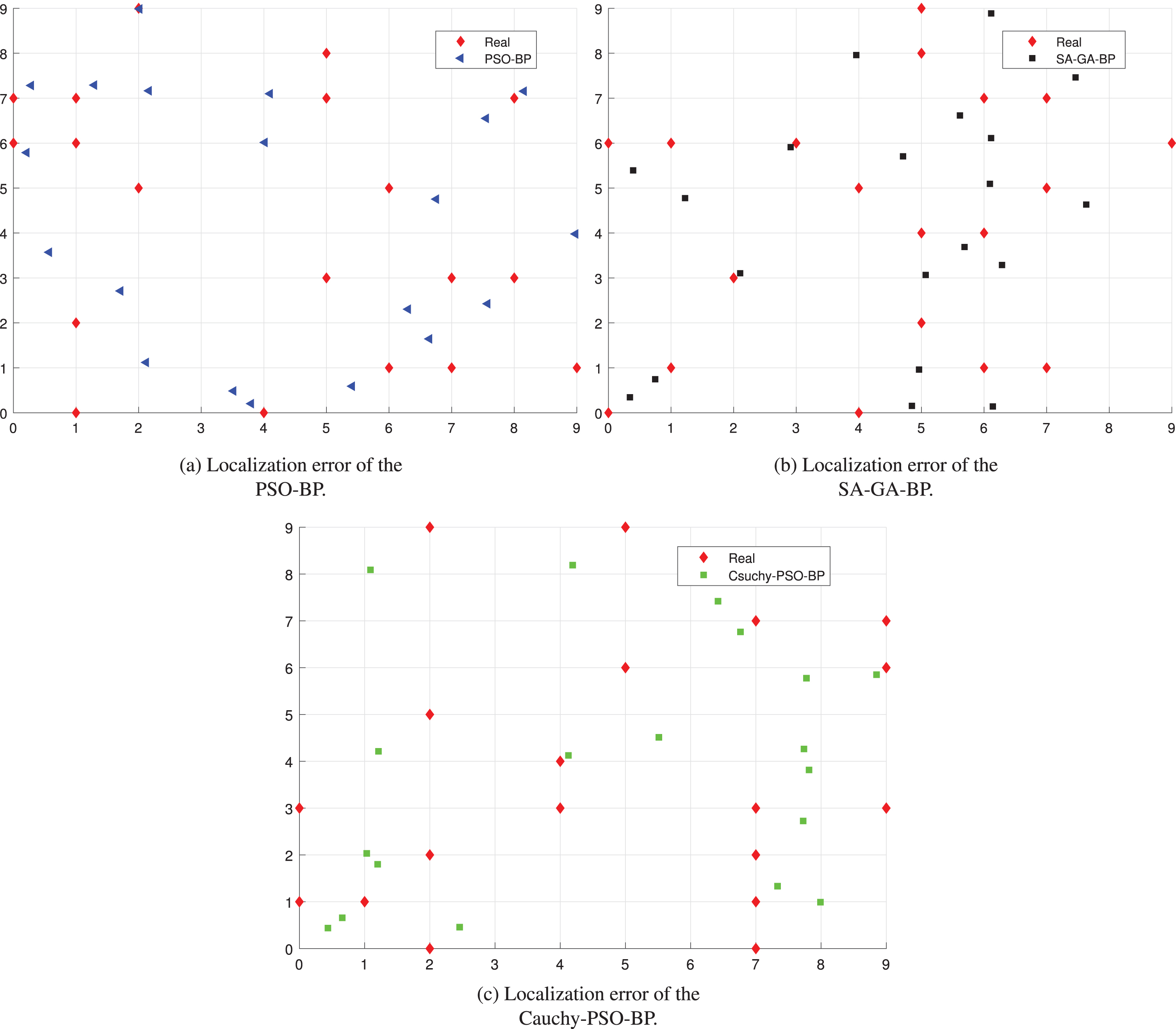
Comparison of location errors of three algorithms.

Fig. 13

PSO-BP, SA-GA-BP and Cauchy-PSO-BP location errors.

Table 3

Comparison of location errors of three algorithms

Algorithm	Maximum error	Minimum error	Average error
PSO-BP	1.943m	0.174m	0.977m
SA-GA-BP	1.644m	0.121m	0.791m
Cauchy-PSO-BP	1.527m	0.089m	0.704m

5.3.3 Efficiency of Csuchy-PSO algorithm

In this paper, the Cauchy mutation theory is introduced into particle swarm optimization, which reduces the iteration times of particle swarm optimization and improves the convergence speed of BPNN. Figure 14 shows the iteration times and corresponding fitness values of PSO, SA-GA and Cauchy-PSO. Table 4 shows the number of iterations and iteration time required to train the BP model. As can be seen from Fig. 14 and Table 4, compared to the SA-GA algorithm, the Cauchy-PSO algorithm requires more iterations, but the required iteration time is almost the same. And based on the fitness value, the Cauchy-PSO algorithm has a lower fitness value, which further avoids local optimization.

Table 4
Comparison of iteration times and training time

PSO-BP SA-GA-BP Cauchy-PSO-BP

Iterations 143 72 114

Fitness Value 1.66×10^-3 1.42×10^-3 1.34×10^-3

Training time 153.3s 116.6s 125.7s

PSO-BP	SA-GA-BP	Cauchy-PSO-BP
Iterations	143	72	114
Fitness Value	1.66×10^-3	1.42×10^-3	1.34×10^-3
Training time	153.3s	116.6s	125.7s

Fig. 14

Iterative curves of PSO-BP, SA-GA-BP and Cauchy-PSO-BP algorithms.

5.4 Ablation experiment based on AI-Cauchy-PSO algorithm

Since the adaptive positioning structure may train BPNN many times in the positioning process, the speed of training BPNN is the key factor of positioning efficiency. Applying PCA to reduce the dimension of data is an important means to improve the training speed of BPNN. According to PCA test performance experiment, the training speed of BPNN is obviously improved after dimensionality reduction of data. Aiming at the shortcomings of BPNN, using Cauchy mutation particle swarm optimization algorithm to optimize BPNN can effectively reduce the positioning error. However, when the indoor environment changes, it is difficult to reduce the positioning error only by optimizing BPNN with optimization algorithm. Changing BPNN to adapt to the current environment is the most effective way to reduce the positioning error. Figure 15 shows the positioning errors of BP, Cauchy-PSO-BP, AI-BP and AI-Cauchy-PSO-BP in different time periods, where AI-BP is an adaptive BP positioning model and AI-Cauchy-PSO-BP is an adaptive Cauchy particle swarm optimization BP positioning model. Table 5 reveals that the adaptive positioning model can better adapt to the noise changing environment while the BPNN improved by Cauchy-PSO has a smaller positioning error. So the AI-Cauchy-PSO-BP model has both higher positioning accuracy and environmental adaptability.

Fig. 15

Localization errors of different algorithms in different time periods.

Table 5

Comparison of location average errors in different time periods

Algorithm	6:00–8:00	8:00–18:00	18:00–22:00	22:00–6:00
BP	0.742m	1.561m	1.206m	0.684m
Cauchy-PSO-BP	0.473m	1.044m	0.991m	0.4378m
AI-BP	0.746m	1.187m	0.961m	0.419m
AI-Cauchy- PSO-BP	0.502m	0.855m	0.772m	0.301m

6 Conclusion

To make the BPNN localization algorithm have stronger adaptability and higher localization accuracy, this paper improves the traditional BPNN localization algorithm from two aspects and compared with the existing algorithms.

Traditional BPNN localization algorithm has limited adaptability in the environment with constantly changing noise. Aiming at the problems, an adaptive BPNN localization structure is proposed. The simulation results show that the adaptive positioning algorithm can effectively compensate for this shortcoming. Compared with the existing positioning algorithms, the adaptive positioning algorithm has higher positioning accuracy in the environment of noise change.

Aiming at the problem that BP is easy to fall into the local optimal solution, Cauchy-PSO algorithm is combined with BPNN and applied to personnel positioning. The algorithm optimizes the initial weight and threshold of BPNN, which can further avoid the local optimal problem.

In addition, aiming at the problem that fingerprint database will produce “high-dimensional disaster” and the training speed of BPNN is slow, PCA is used to select and reduce the dimension of AP features. This method can not only make RSSI value in fingerprint database have uniform low-dimensional characteristics, but also meet the demand of adaptive positioning structure for BPNN training speed.Based on the above experiments, this paper analyzes the evaluation indexes such as positioning accuracy, operation efficiency and convergence speed of the improved positioning algorithm. Experimental results show that the algorithm has high positioning accuracy in the environment of changing noise intensity. This paper provides a development idea for the future indoor personnel positioning algorithm.

Footnotes

Acknowledgment

We are grateful to the Project of Young YuYou of North China University of Technology, 2018 and the Research on Key Technologies of accurate positioning of BINGTUAN transportation key vehicles and infrastructure based on Beidou under Grant 2108AB028.

References

Jiang

, Li

, Zhao

and Ou

, A distributed localizationalgorithm for large scale sensor networks, Acta Electron Inf 41 (2019), 3022–3028.

Rizk

, Torki

and Youssef

, CellinDeep: Robust and accuratecellular-based indoor localization via deep learning, IEEESensors J 19(2019), 2305–2312.

Hernandez

S.M.

and Bulut

, Using perceived direction informationfor anchorless relative indoor localization, J Netw ComputAppl 165 (2020), 102714.

Tiwari

and Jain

V.K.

, HILS: Hybrid indoor localisation systemusing Wi-Fi received signal strength and inertial sensor’smeasurements of smart-phone, IET Commun 13 (2019), 1595–1606.

Yen

H.-C.

, Ou Yang

L.-Y.

Tsai

Z.-M.

, 3-D Indoor Localization andIdentification Through RSSI-Based Angle of Arrival Estimation WithReal Wi-Fi Signals, IEEE Transactions on Microwave Theory andTechniques 70 (2022), 4511–4527.

Xie

, Jiang

, Zhao

and Zhang

, A Wi-Fi-based wirelessindoor position sensing system with multipath interferencemitigation, Sensors 19 (2019), 3983.

Sabale

, Sapre

and Mini

, Obstacle Handling Mechanism forMobile Anchor Assisted Localization in Wireless Sensor Networks, IEEE Sensors Journal 19 (2021), 21999–22010.

Yang

, Guo

, Zhao

and Zhao

, A Novel TrilaterationAlgorithm for RSSI-Based Indoor Localization, IEEE SensorsJournal 14 (2020), 8164–8172.

Hoang

M.T.

et al. A Soft Range Limited K-Nearest NeighborsAlgorithm for Indoor Localization Enhancement, IEEE SensorsJournal 24 (2018), 10208–10216.

10.

Yoo

, Change Detection of RSSI Fingerprint Pattern for IndoorPositioning System, IEEE Sensors Journal 5 (2019), 2608–2615.

11.

Hoang

M.T.

, Yuen

, Dong

, Lu

, Westendorp

and ReddyRecurrent

, Neural Networks for Accurate RSSI Indoor Localization, IEEE Internet of Things Journal 6 (2019), 10639–10651.

12.

Belmonte-Hernández

, Hernández-Peñaloza

, Martín Gutiérrez

Álvarez

, Recurrent Model forWireless Indoor Tracking and Positioning Recovering Using GenerativeNetworks, IEEE Sensors Journal 6 (2020), 3356–3365.

13.

Munadhil

, Gharghan

S.K.

, Mutlag

A.H.

, Al-Naji

and ChahlNeural

, Network-Based Alzheimer’s Patient Localization for WirelessSensor Network in an Indoor Environment, IEEE Access 8(2020), 150527–150538.

14.

Gharghan

S.K.

, Nordin

, Ismail

and Ali

J.A.

, Accurate WirelessSensor Localization Technique Based on Hybrid PSO-ANN Algorithm forIndoor and Outdoor Track Cycling, IEEE Sensors Journal 16 (2016), 529–541.

15.

Soro

and Lee

, Joint Time-Frequency RSSI Features forConvolutional Neural Network-Based Indoor FingerprintingLocalization, IEEE Access 7 (2019), 104892–104899.

16.

Liu

, Li

and Li

, Indoor mobile positioning technology basedon BP artifificial neural network, Mod. Electron. Technol 42 (2019), 25–28.

17.

Xie

, Wang

and Huan

, BPNN Based Indoor FingerprintingLocalization Algorithm Against Environmental Fluctuations, IEEESensors Journal 22 (2022), 12002–12016.

18.

Lin

, Yu

, Hao

, Wang

and Bu

, An Indoor Wi-FiLocalization Algorithm Using Ranging Model Constructed WithTransformed RSSI and BP Neural Network, IEEE Transactions onCommunications 70 (2022), 2163–2177.

19.

Alsmadi

, Kong

, Sandrasegaran

and Fang

, An ImprovedIndoor Positioning Accuracy Using Filtered RSSI and Beacon Weight, IEEE Sensors Journal 21 (2021), 18205–18213.

20.

Eberechukwu

, Park

, Laoudias

, Horsmanheimo

and KimSmartphone-Based

, Indoor Localization via Network Learning WithFusion of FTM/RSSI Measurements, IEEE Networking Letters 5 (2023), 21–25.

21.

Alsmadi

, Kong

, Sandrasegaran

and Fang

, An ImprovedIndoor Positioning Accuracy Using Filtered RSSI and Beacon Weight, IEEE Sensors Journal 21 (2021), 18205–18213.

22.

Wang

, Zhu

, Wang

, Zhao

and Yang

, Research on IndoorPositioning Algorithm Based on SAGA-BP Neural Network, IEEESensors Journal 22 (2022), 3736–3744.

23.

Bian

, Huang

, Wang

and Yu

, Wireless sensor networkpositioning optimization based on PSO-BP algorithm, Telecommun.Technol 57 (2017), 139–144.

24.

Lin

, Yu

, Hao

, Wang

and Bu

, An Indoor Wi-FiLocalization Algorithm Using Ranging Model Constructed WithTransformed RSSI and BP Neural Network, IEEE Transactions onCommunications 70 (2022), 2163–2177.

25.

Liu

, Huang

, Sun

, Yu

and Xiao

, Data Fusion forMulti-Source Sensors Using GA-PSO-BP Neural Network, IEEETransactions on Intelligent Transportation Systems 22 (2021), 6583–6598.

26.

Xia

, Chen

and Xu

, Multiview PCA: A Methodology of FeatureExtraction and Dimension Reduction for High-Order Data, IEEETransactions on Cybernetics 52 (2022), 11068–11080.

27.

Zubair

et al. Detection of Epileptic Seizures From EEG Signalsby Combining Dimensionality Reduction Algorithms With MachineLearning Models, IEEE Sensors Journal 21 (2021), 16861–16869.

28.

JankovÁ

and van de Geer

, De-Biased Sparse PCA: Inferencefor Eigenstructure of Large Covariance Matrices, IEEETransactions on Information Theory 67 (2021), 2507–2527.

29.

Qin

, Liu

, Wang

, Shi

and Hu

, Indoor visible lightpositioning algorithm based on double BP neural network, OptCommun Technol 45 (2020), 1–9.

30.

Jain

N.K.

, Nangia

and Jain

, A review of particle swarmoptimization, J Inst Eng (India): B 99 (2018), 407–411.

31.

Men

, Chen

and Zhou

, A Gaussian Type-2 FuzzyProgramming Approach for Multicrowd Congestion-Relieved EvacuationPlanning, IEEE Transactions on Intelligent TransportationSystems 23 (2022), 20978–20990.

32.

Zhao

, Yu

, Fang

, Tian

and Han

, A Path Planning MethodBased on Multi-Objective Cauchy Mutation Cat Swarm OptimizationAlgorithm for Navigation System of Intelligent Patrol Car, IEEEAccess 8 (2020), 151788–151803.

33.

Tian

, Zhao

and Shi

, DMPSO: Diversity-Guided Multi-MutationParticle Swarm Optimizer, IEEE Access 7 (2019), 124008–124025.

34.

Sandoval

R.M.

, Garcia-Sanchez

A.-J.

and Garcia-Haro

, ImprovingRSSI-Based Path-Loss Models Accuracy for Critical Infrastructures: ASmart Grid Substation Case-Study, IEEE Transactions onIndustrial Informatics 14 (2018), 2230–2240.

35.

Wang

, Qingshan

, Maozhen

, Zhaoba

, Zhao

and YanfangA

, Research on the Indoor Rotating Arc Triangle Positioning AlgorithmBased on RSSI, IEEE Access 8 (2020), 223069–223077.

An adaptive indoor localization model based on Cauchy-PSO optimized BPNN

Abstract

Keywords

1 Introduction

3.1 BP neural network (BPNN) model

4.1 Cauchy-PSO algorithm

5 Experiment results and analysis

5.1.1 PCA experiment preparation

5.1.2 Impact of fingerprint database degradation on localization

5.2.1 BP model initialization

5.2.2 Localization error of adaptive BP model and other models

5.3.1 Cauchy-PSO algorithm initialization

5.3.2 Location accuracy of Csuchy-PSO algorithm

Table 4 Comparison of iteration times and training time PSO-BP SA-GA-BP Cauchy-PSO-BP Iterations 143 72 114 Fitness Value 1.66×10-3 1.42×10-3 1.34×10-3 Training time 153.3s 116.6s 125.7s

Footnotes

Acknowledgment

References

Table 4
Comparison of iteration times and training time

PSO-BP SA-GA-BP Cauchy-PSO-BP

Iterations 143 72 114

Fitness Value 1.66×10^-3 1.42×10^-3 1.34×10^-3

Training time 153.3s 116.6s 125.7s