Modified suppressed relative entropy fuzzy c-means clustering algorithm

Abstract

The Fuzzy C-means (FCM) algorithm is one of the most widely used algorithms in unsupervised pattern recognition. As the intensity of observation noise increases, FCM tends to produce large center deviations and even overlap clustering problems. The relative entropy fuzzy C-means algorithm (REFCM) adds relative entropy as a regularization function to the fuzzy C-means algorithm, which has a good ability for noise detection and membership assignment to observed values. However, REFCM still tends to generate overlapping clusters as the size of the cluster increases and becomes imbalanced. Moreover, the convergence speed of this algorithm is slow. To solve this problem, modified suppressed relative entropy fuzzy c-means clustering (MSREFCM) is proposed. Specifically, the MSREFCM algorithm improves the convergence speed of the algorithm while maintaining the accuracy and anti-noise capability of the REFCM algorithm by adding a suppression strategy based on the intra-class average distance measurement. In addition, to further improve the clustering performance of MSREFCM for multidimensional imbalanced data, the center overlapping problem and the center offset problem of elliptical data are solved by replacing the Euclidean distance in REFCM with the Mahalanobis distance. Experiments on several synthetic and UCI datasets indicate that MSREFCM can improve the convergence speed and classification performance of the REFCM for spherical and ellipsoidal datasets with imbalanced sizes. In particular, for the Statlog dataset, the running time of MSREFCM is nearly one second less than that of REFCM, and the accuracy of MSREFCM is 0.034 higher than that of REFCM.

Keywords

Fuzzy c-means clustering relative entropy fuzzy c-means clustering modified suppressed relative entropy fuzzy c-means Mahalanobis distance

1 Introduction

Pattern recognition theory is a data analysis method that uses computer technology to study sample data without assuming any mathematical model. It consists of two different methods: supervised clustering and unsupervised clustering. Compared to supervised classification, unsupervised classification methods are often more effective in practical problem. In unsupervised classification, the objective is to identify natural groupings within the sample data, assuming that each data point can belong to more than one class. In reality, data points may belong to more than one cluster. Zadeh successfully introduced fuzzy logic to handle this uncertainty, which has made significant strides in cluster analysis. This article focuses on studying clustering problems, particularly in the application of fuzzy clustering methods. Many fuzzy clustering methods have been developed ([1 –6]), which utilize fuzzy set theory to partition observational data into multiple clusters. Fuzzy clustering has found applications in various fields such as image segmentation ([7, 8]), weather forecasting [9], medical diagnosis [10], etc. So far, the FCM (fuzzy c-means) algorithm has provided a logical and accurate approach to clustering data [11].

According to the analysis in [12], as the dataset size increase, the computation time of the FCM algorithm increases rapidly. In other words, although the FCM algorithm provides better division quality, it comes at the cost of a slow convergence rate. To address this issue and accelerate the calculation of FCM, the suppressed Fuzzy C-means algorithm (S-FCM) was introduced in reference [4]. This algorithm aims to improve the convergence speed of FCM while maintaining its high classification accuracy. The key step in this algorithm is the selection of an appropriate suppression rate to achieve practical applications. Selecting the proper parameters is crucial as it significantly impacts the performance of clustering algorithms. To address this challenge, several parameter selection schemes have been proposed by scholars ([13 –17]).

Furthermore, FCM is a partitioning algorithm that divides observations into C partitions regardless of the presence of noise in the observational data. However, it is common for all clusters to have low membership for noise points. Probabilistic C-means clustering (PCM) can overcome this problem. In the PCM algorithm, there is no interaction between clusters, leading to clustering centers in the PCM algorithm being very close or even overlapping. Additionally, the PCM clustering algorithm lacks much flexibility, and the algorithm needs quite good information to converge to the global minimum. In the literature on fuzzy clustering, many other methods attempt to alleviate the weakness of FCM by adding a regularization function to its objective function. Quadratic regularization [18], adaptive loss regularization [19], symmetric relative entropy [20], and fractional entropy [21] are some well-known regularization functions.

Relative entropy is a measure of the distance between two distributions, and it is commonly used to quantify the degree of dissimilarity between clusters. Furthermore, the relative entropy is a convex function that has been applied as a regularization function in FCM by several researchers, including Z.F. Hao et al. [20], J. Bonilla et al. [22], and F. Salehi et al. [23]. To improve FCM and PCM, Zarinbal et al. introduced relative entropy into the objective function of FCM as a regularization term, resulting in the development of the relative entropy fuzzy c-means (REFCM) clustering algorithm [24]. The REFCM is to minimize the intra-cluster distances while simultaneously maximizing the inter-cluster differences. However, it’s worth noting that the REFCM algorithm is associated with high computational complexity and slow convergence. Furthermore, as the number of clusters increases or when the cluster sizes vary significantly, the REFCM algorithm may exhibit the issue of overlapping cluster centers. Aiming at this problem, this paper proposes modified suppression relative entropy fuzzy C-means clustering (MSREFCM). In selecting the suppression rate, MSREFCM takes into account the impact of each iteration’s results on the suppression rate. Additionally, the MSREFCM algorithm introduces a suppression scheme that incorporates the intra-class mean distance as a selection strategy. Moreover, it utilizes Mahalanobis distance to enhance its applicability to diverse types of data. The proposed method has been tested in multiple experiments and compared with five widely clustering algorithms: FCM [1], S-FCM [4], MSFCM [5], PCM [3], and REFCM [24].

The rest of this paper is arranged as follows: Section 2 presents in sequence the FCM, S-FCM, MSFCM, PCM, and REFFCM algorithms. Section 3 discusses the proposed MSREFCM algorithm. Section 4 discusses the computational complexity and performance of the MSREFCM algorithm. Finally, Section 5 reports conclusions.

2 Preliminaries

FCM and PCM algorithms are widely utilized in unsupervised learning to recognize patterns in data. The REFCM algorithm adds relative entropy as a regularization function to the FCM model, which improves its capabilities to deal with noise. S-FCM and MSFCM algorithms adopt a competitive learning mechanism. However, these algorithms can be susceptible to significant center deviations or clustering issues with overlapping clusters as the intensity of noise increases. This section provides a concise overview of the models used by the five algorithms.

2.1 FCM algorithm

As one of the most popular clustering algorithms, the objective function of FCM [25] is shown in Equation (1), and the constraints are shown in Equation (2).

$min J (U, V, c) = \sum_{i = 1}^{c} \sum_{j = 1}^{N} u_{ij}^{m} d_{ij}^{2}$ (1) S.t

${\begin{matrix} \sum_{i = 1}^{c} u_{ij} = 1 \forall j \in {1, \dots \dots N} \\ u_{ij} \in [0, 1] \forall i, j \\ 0 < \sum_{j = 1}^{N} u_{ij} \forall i \in {1, \dots \dots c} \end{matrix}$ (2)

Where u_ij is the degree of membership of jth observation in ith cluster, $d_{ij}^{2}$ is the Euclidean distance of jth observation from the center of ith cluster, m is the degree of fuzziness, and c and N are clusters and observations, respectively.

2.2 S-FCM algorithm

Fan et al. proposed the S-FCM algorithm to overcome the slow convergence speed of FCM. In the S-FCM algorithm, the maximum membership degree is rewarded, and the non-winning membership degree is suppressed. This modification can maintain the original order of membership values between clusters. The modification of membership degree is shown in Equation (3).

$u_{pj} = 1 - α \sum_{i \neq p} u_{ij} = 1 - α + α u_{pj}$ (3)

u_pj has the largest membership of all groups, and u_ij = αu_ij, i ≠ p, where 0 ≤ α ≤ 1.

2.3 MSFCM algorithm

Since the suppression factor in the S-FCM algorithm is fixed, the performance of S-FCM may be significantly reduced if the parameter α is not correctly selected. To solve this problem, Hung et al. proposed an MSFCM algorithm that can automatically select the appropriate suppression parameters based on the prototype-driven learning method. The selection of the suppression parameter given by them is shown in Equation (4).

$α = exp (- min_{i \neq k} \frac{{∥ v_{i} - v_{k} ∥}^{2}}{β})$ (4)

Where $β = \frac{\sum_{j = 1}^{N} {∥ x_{j} - \bar{x} ∥}^{2}}{N}$ and $\bar{x} = \frac{\sum_{j = 1}^{N} x_{j}}{N}$ . β is a sample variance.

2.4 PCM algorithm

1993 Keller et al. [3] Combining possibilistic theory, the possibilistic c-means clustering algorithm was obtained by abandoning the FCM constraint. It only needs $max_{i} t_{ij} > 0$ .

The objective function is shown in Equation (5).

$min J (T, V, c) = \sum_{i = 1}^{c} \sum_{j = 1}^{N} t_{ij}^{m} d_{ij}^{2} + \sum_{i = 1}^{c} η_{i} \sum_{j = 1}^{N} {(1 - t_{ij})}^{m}$ (5)

Where η_i is a positive number or a penalty factor. Other parameters have the same definitions as before.

2.5 REFCM algorithm

To overcome the shortcomings of FCM that its performance deteriorates when the noise of the observation result is large, Zarinbal et al. added relative entropy [26] to the objective function of FCM as the regularization function and proposed the REFCM algorithm [24], whose objective function is shown in Equation (6).

$\begin{matrix} min J (U, V, c) = \sum_{i = 1}^{c} \sum_{j = 1}^{N} u_{ij}^{m} d_{ij}^{2} \\ - θ \sum_{j = 1}^{N} \sum_{i = 1}^{c} \sum_{\begin{matrix} k = 1 \\ k \neq i \end{matrix}}^{c} u_{ij} ln (\frac{u_{ij}}{u_{kj}}) \end{matrix}$ (6)

Where θ is the positive coefficient of relative entropy, which determines the degree of influence of relative entropy. The definition of other parameters is the same as before.

Considering W₀ (·) as the principle branch of the Lambert-W function, the degree of membership of this observation in ith cluster, u_ij, and the center point of ith cluster, v_i, are obtained by Equations (7) and (8), respectively [24]:

$u_{ij} = {({(\frac{\frac{- m (m - 1) d_{ij}^{2}}{θ}}{W_{0} [\frac{- m (m - 1) d_{ij}^{2}}{θ} \exp (- (m - 1) (\frac{λ_{j} - θ \sum_{\begin{matrix} k = 1 \\ k \neq i \end{matrix}}^{c} ln (u_{kj}) + θ}{θ}))]})}^{1 / m - 1})}^{- 1}$ (7)

$v_{i} = \frac{\sum_{j = 1}^{N} u_{ij}^{m} x_{j}}{\sum_{j = 1}^{N} u_{ij}^{m}}$ (8)

Where λ_j, j = 1, …… , N is the Lagrange multiplier, its formula is shown in Equation (9), and the definitions of other parameters are the same as before.

$\begin{matrix} λ_{j} \geq \max {\frac{θ}{m - 1} (ln (\frac{m (m - 1) d_{ij}^{2}}{θ}) + 1) + θ \sum_{\begin{matrix} k = 1 \\ k \neq i \end{matrix}}^{c} ln (u_{kj}) - θ, {md}_{ij}^{2} + θ \sum_{\begin{matrix} k = 1 \\ k \neq i \end{matrix}}^{c} ln (u_{kj}) - θ} \end{matrix}$ (9)

With this declaration, since the REFCM algorithm can assign low membership to all clusters of noise points, the sum of membership at the noise point is less than 1. Since λ_j is calculated based on the boundary in the equation, there is no specific membership scheme. Therefore, the $\sum_{i = 1}^{c} u_{ij} = 1$ constraint condition may not satisfy some observations, which are reflected in the experiment.

3 The proposed MSREFCM algorithm

3.1 The strategy of suppression behavior

Considering that different regional data will have other effects on clustering results, a more stable suppressive competitive learning algorithm is proposed. The key concept behind this approach is as follows: if the distance between a data point and its cluster center is less than K times the average intra-class distance between the sample and its cluster center, the data point is considered to be in the cluster core, and then the reward measure is performed. On the other hand, if the distance from the data point to the cluster center is greater than K times the average intra-class distance between the sample and the cluster center, it means that the sample does not belong to the cluster core and is suppressed. The average intra-class distance between classes is as follows:

${\hat{d}}_{i} = \frac{\sum_{j = 1}^{N} u_{ij} d_{ij}}{\sum_{j = 1}^{N} u_{ij}}$ (10)

Where ${\hat{d}}_{i}$ represents the total average intra-class distance between all samples and cluster center i.

Next, two examples are given to briefly intro-duce the intra-class average distance metric. The number of data points generated is 800 and 1000, respectively, and the number of noise points is 200. The Gaussian radius of the first example is 0.4, and the Gaussian radius of the second example is 0.6. As shown in Fig. 1. In both images, the inner circle represents the \hfilneg circle drawn with the average distance within the class as the radius. The outer circle represents the circle drawn with the cluster kernel as the radius. The radius of the outer circle in Fig. 1 (a) is 1.5 times that of the inner circle, and the radius of the outer circle in Fig. 1 (b) is two times that of the inner circle.

Fig. 1

The radius of the core in (a) is 1.5 times the mean distance within the class, and the radius of the core in (b) is two times the mean distance within the class.

In addition, in the initial iteration, the average distance within the class is larger, the clustering kernel is larger, and the data clustering within the clustering kernel will compete for comparison, thus rewarding the winning membership and punishing the non-winning membership. As iteration progresses, the average distance within the class gradually decreases, and the clustering kernel gradually decreases until the clustering center is correctly located. The clustering kernel finds most of the corresponding data and gradually eliminates noise interference.

3.2 The MSREFCM algorithm

In this paper, we have introduced the intra-class average distance metric to mitigate the shift of the cluster center caused by noise points. Furthermore, we have proposed the concept of a clustering kernel to identify the core data of each class and facilitate the rewarding of winning membership degrees while punishing non-winning membership degrees. This approach actively attracts the center and enhances the iteration speed of the algorithm. At the same time, it avoids the unreasonable correction of the membership degree of close-range noise and enhances the robustness of the algorithm.

In addition, if the α value is incorrect, the corrected maximum membership value may be greater. For multi-class clustering, the clustering center is easy to deviate from, which is obviously inappropriate. As a result, we employed the suppression strategy of selecting suppressor α [13] based on the data distribution structure. The key idea of the selection process is to use the clustering validity function to determine the α parameter, which makes the suppression scheme more reasonable. The formula for selecting α according to the data distribution structure is shown in Equation (11).

$α = \frac{1}{log c} (- \frac{1}{n} \sum_{i = 1}^{c} \sum_{j = 1}^{N} u_{ij} log u_{ij})$ (11)

For the X ={ x₁, …, x_n } dataset, the fuzzy partition entropy [32] is defined as $H (U) = - \frac{1}{n} \sum_{i = 1}^{c} \sum_{j = 1}^{N} u_{ij} log u_{ij}$ . It can be seen that H (U) has the following conclusion: when the classification is a hard partition, H (U) is 0, and when the classification is a maximum fuzzy partition, H (U) is log c. Therefore, the suppression rate α selected according to the data distribution structure can be regarded as an increasing function of fuzzy partition entropy. That is, using the clustering validity function to determine parameter α makes the suppression scheme more reasonable.

In addition, the Euclidean distance metric used in FCM and PCM is only applicable to clustering spherical or elliptical data sets. To improve the universality of FCM, Gustafson et al. proposed the Gustafson-Kessel clustering (GK) ([33 –35]) algorithm, which uses Mahalanobis distance instead of Euclidean distance in FCM. The Mahalanobis distance calculation formula is shown in Equation (12). The GK algorithm is more suitable for ellipsoid and linear data sets than the FCM algorithm. Therefore, we replace Euclidean distance in the REFCM algorithm with Mahalanobis distance.

$d_{ij} = {(x_{j} - v_{i})}^{T} A_{i} (x_{j} - v_{i})$ (12)

Where A_i is positive definite and det(A_i) = r_i, r_i > 0, it is a norm matrix describing the shape of cluster v_i. $A_{i} = {(r_{i} \det (S_{i}))}^{\frac{1}{S}} S_{i}^{- 1}$ , $S_{i} = \frac{\sum_{j = 1}^{N} u_{ij}^{m} (x_{j} - v_{i}) {(x_{j} - v_{i})}^{T}}{\sum_{j = 1}^{N} u_{ij}^{m}}$ , where S_i is the fuzzy covariance matrix of cluster β_i = (v_i, A_i).

Therefore, the MSREFCM clustering algorithm proposed in this paper can use the competitive learning mechanism to change the membership value in each iteration. As shown in Equation (13).

$u_{ij} = {\begin{matrix} 1 - α \sum_{i \neq p} u_{ij} = 1 - α + α u_{pj}, if d_{ij} \leq K d_{i} \\ α u_{ij}, i \neq p or if d_{ij} \geq K d_{i} \end{matrix}$ (13)

The fuzzy membership is modified by Equation (13) so that the membership value of all non-winners is multiplied by a so-called suppression rate α (0 ≤ α ≤ 1), and the winner’s membership increases accordingly. When α = 0, MSREFCM becomes an algorithm similar to HCM. When α = 1, the MSREFCM and REFCM algorithms are consistent.

Furthermore, the MSREFCM method employs the Mahalanobis distance. The proof of this theorem can be found in Appendix A.

MSREFCM clustering algorithm:

Step 1: Fix the number of clusters c (2 ≤ c ≤ N), the degree of fuzziness m, and the relative entropy coefficient θ.

Step 2: Determine the initial membership u⁽⁰⁾ and the center point v⁽⁰⁾, setting L = 0. Repeat the following steps until $(u_{ij}^{(L - 1)} - u_{ij}^{(L)} \leq ɛ)$ .

Step 3: Update d_ij by Equation (12).

Step 4: Update λ_j by Equation (9).

Step 5: Update u^(L) by Equation (7).

Step 6: Modify u^(L) by Equations (11) and (13).

Step 7: Update v^(L) by Equation (8).

Step 8: Increment L.

The flowchart of MSREFCM is shown in Fig. 2.

Fig. 2

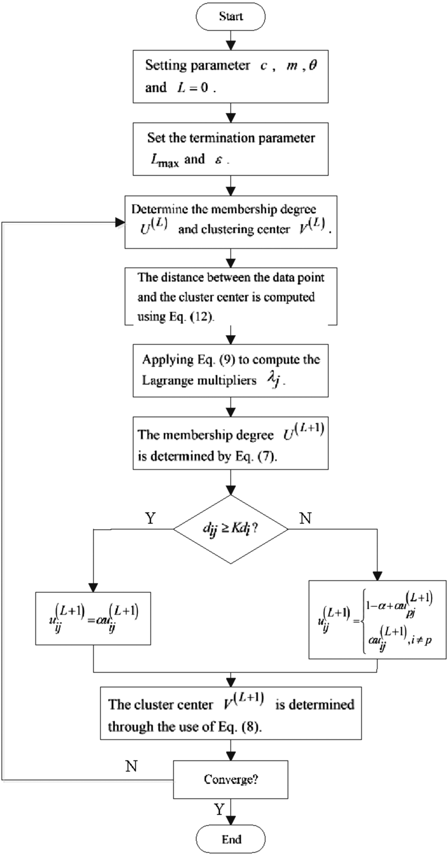
The flowchart of MSREFCM.

3.3 Analysis of the suppression behavior of MSREFCM algorithm

In the previous paper [4], the cluster with the most significant membership value of sample x_j among all clusters is denoted as pth cluster, and pth cluster is regarded as the winner cluster, so the membership degree of sample x_j belonging to cluster p is represented as u_pj. In this paper, the sample x_j belongs to the cluster within the cluster kernel, which is denoted by the winner pth cluster, and its membership degree is expressed as u_pj. The other clusters are called non-winning clusters, and the degree of membership of the observed value x_j to the non-winning cluster is denoted u_ij, i ≠ p.

In the suppression strategy, we introduced the concept of clustering kernels to identify the core data of each cluster, rewarding in data in the kernel dominating and other data being punished. The membership degree of the non-winning cluster data is proportionally suppressed by the product of α, while the membership degree of the winning cluster data is amplified. According to Equations (7) and (9), the relationship between sample x_j and membership degree is not only related to the distance from cluster center v_i to sample x_j, but also to the Lambert-W function value of the distance from sample x_j to cluster i. The built-in Lambert-W function can be denoted $f = max {- \frac{1}{e}, \frac{- m (m - 1) d_{ij}^{2}}{θ} exp (\frac{- m (m - 1) d_{ij}^{2}}{θ})}$ . When the value of the Lambert function is -raise0.7ex1 / lower0.7exe, the membership degree is inversely proportional to the distance. Specifically, when the Lambert function takes $\frac{- m (m - 1) d_{ij}^{2}}{θ} exp (\frac{- m (m - 1) d_{ij}^{2}}{θ})$ , the membership degree can be expressed as $u_{i j} = {(\exp (\frac{- m (m - 1) d_{i j}^{2}}{θ}))}^{1 / m - 1}$ , indicating that the membership degree u_ij is inversely proportional to the distance d_ij. Therefore, it can be simply considered that the relationship between sample x_j and membership degree is only related to the distance from cluster center v_i to sample x_j.

As shown in Fig. 3, where v₁, v₂ and v₃ are the centers of the three clusters. The observed value x_j is within the cluster core of the cluster center v₁ (the blue circle represents the cluster core of v₁), and outside the cluster core of the cluster centers v₂ and v₃, then the winner cluster is v₁. At this time, the membership of the winner cluster will be rewarded, that is, the distance d_1j from x_j to v₁ should be shortened to $d_{1 j}^{'}$ . For non-winner clusters v₂ and v₃, their degree of membership should be multiplied by α to obtain a penalty, corresponding to the distance from sample x_j to clusters v₂ and v₃, and the distance from d_2j and d_3j should be extended to $d_{2 j}^{'}$ and $d_{3 j}^{'}$ . At this time, for sample x_j, the distance of the non-winner cluster increases, indicating that the membership difference between the winner cluster and the non-winner cluster increases, and the inter-cluster relationship is introduced. In this case, the convergence of the original data points to the nearest cluster can be made faster, and the number and time of iterative updates can be shortened accordingly.

Fig. 3

The effect of suppression behaviour in MSREFCM.

4 Experimental results

In Section 4.1, we introduce the complexity of FCM, S-FCM, PCM, MSFCM, REFCM, and the MSRFCM algorithm proposed in this paper, along with the parameter settings and running environment of the algorithm. In Section 4.2, we verify the effectiveness of the proposed algorithm using 8 synthetic datasets, 2 UCI datasets, and 2 image datasets.

4.1 Performance evaluation

Kolen and Hutcheson mentioned that FCM is asymptotically running in time O (Nc²p) [27], where N is the number of p-dimensional observations and c is the number of clusters. The computational complexity of PCM algorithm is O (Nc²p) The computational complexity of the S-FCM algorithm and the MSFCM algorithm is O (Nc²p) + O (2Nc). The computational complexity of the REFCM algorithm obtained by adding relative entropy to FCM is O (Nc²p) + O (2Nc log(Nc)). In addition, the overall complexity of the MSREFCM clustering method proposed in this paper is O (Nc²p) + O (2Nc log(Nc)) + O (2Nc). Therefore, compared with FCM, S-FCM, MSFCM, and REFCM methods, although the proposed method increases the complexity of the algorithm, the idea of competitive learning improves the convergence speed and reduces the running time.

Under different data conditions, the MSREFCM algorithm will be compared with the FCM, S-FCM, PCM, MSFCM, and REFCM algorithms. These clustering methods have the following properties: (1) FCM, m = 2, (2) S-FCM, m = 2.5, α = 0.5, (3) PCM, m = 2.5, (4) MSFCM, m = 2.5, β = 0.005, (5) REFCM, m = 2.5, θ = 1.5, (6) MSREFCM, m = 2.5, θ = 1.5. To measure and compare the ability of the proposed methods to identify accurate results, the Kwon validity measure V_k (c) [28], Separation coefficient V_SC [29], Partition coefficient and exponential separation V_PCAEC [30], the overall F-measure for the entire data set F^*, the normalized mutual information NMI, and the adjusted Rand index ARI [31], accuracy, iteration number, and computing time criteria are applied.

The smaller the V_k (c) and V_SC values, the better. The V_PCAEC index describes the compactness and separation of clusters by the fuzzy membership function and the relative value of the central distance of an exponential structure. F^*, NMI, and ARI measure how well the two data distributions match. The higher the value of V_PCAEC, F^*, NMI, and ARI, the better. In addition, we tested this model on a system with 8 processors, 16.0 GB of RAM, and a 512 GB SSD, and the CPU frequency is 2.90 GHz.

4.2 Experiments

In this section, the first eight experiments are synthetic datasets, the ninth and tenth experiments are UCI datasets, and the last two experiments are image datasets. In the experiment on the synthetic datasets, we verified that MSREFCM has lower convergence times and higher classification accuracy through Experiments 1 and 2. Additionally, REFCM still tends to produce overlapping clusters as the cluster size increases and the cluster size imbalance increases. Experiments 3, 4, and 5 confirm that MSREFCM can obtain more accurate cluster centers. Experiments 6 and 7 reflect the advantage of the Mahalanobis distance from the structure of the data itself, which makes MSREFCM more robust. Experiment 8 analyzed the effect of suppression factors and fuzzy degrees on membership by classifying simple two-dimensional elliptical datasets. Secondly, for real-world datasets, evaluation metrics are used to assess the effectiveness of the proposed algorithm on the UCI dataset, and the final classification result graph is used to verify the better classification performance of the proposed algorithm on the image dataset.

4.2.1 Synthetic datasets

(Experiment 1) The first experiment involved two well-separated clusters containing a total of 16 data points. As shown in Fig. 4, these data points are numbered from left to right and from top to bottom, with the eighth and ninth data points being noise points. Figure 5(a)–(f) is the membership degree of each data point obtained by FCM, SFCM, PCM, MSFCM, REFCM, and MSREFCM, respectively. The values of the Kwon validity measure, F^*, NMI, ARI, accuracy, iteration number, and computing time criteria are reported in Table 1. The final results are represented by the mean and standard deviation of the ten test data points.

Fig. 4

simple numerical data set.

Fig. 5

Membership degrees obtained by applying (a) FCM, (b) S-FCM, (c)PCM, (d) MSFCM, (e) REFCM, (f) MSREFCM methods for the Experiment 1.

Table 1

The average performance comparison of different algorithms in Experiment 1 (standard deviation in bracket)

	FCM	S-FCM	PCM	MSFCM	REFCM	MSREFCM
V_k (2)	2.741(±0.001)	2.740(±0.001)	2.064(±0.001)	2.355(±0.001)	1.446(±0.001)	1.446(±0.001)
V _SC	0.004(±0.001)	0.003(±0.001)	0.030(±0.042)	0.004(±0.005)	3e-4(±0.001)	2.5e-4(±0.001)
V _PCAEC	1.264(±0.001)	1.412(±0.001)	0.197(±0.278)	0.282(±0.269)	0.394(±0.001)	0.472(±0.282)
F ^*	0.866(±0.001)	0.866(±0.001)	0.866(±0.001)	0.866(±0.001)	0.875(±0.001)	0.950(±0.038)
NMI	0.763(±0.001)	0763(±0.001)	0.763(±0.001)	0.763(±0.001)	0.771(±0.001)	0.828(±0.154)
ARI	0.821(±0.001)	0.821(±0.001)	0.821(±0.001)	0.821(±0.001)	0.823(±0.001)	0.833(±0.137)
Accuracy	0.875(±0.001)	0.875(±0.001)	0.875(±0.001)	0.875(±0.001)	0.875(±0.001)	0.875(±0.001)
Iteration number	10.5(±0.707)	10(±0.001)	45(±0.001)	20(±0.001)	12(±1.414)	14(±0.001)
Computing time(s)	0.010(±0.002)	0.014(±0.002)	0.021(±0.003)	0.026(±0.002)	0.030(±0.002)	0.028(±0.002)

First, observe the membership graphs of these six algorithms in Fig. 5. Among them, the 8th and 9th data points are noise points, and the membership degrees of the FCM clustering algorithm at these two noise points are both 0.5, which indicates that the distances between these two noise points and the two clustering centers are consistent. FCM cluster centers are [3.343, 3.307] and [14.66, 3.307], and the errors between them and cluster centers [3, 3] and [15, 3] previously set are $δ_{1}^{FCM} = 0.454$ and $δ_{2}^{FCM} = 0.458$ . This is due to FCM’s poor robustness and sensitivity to noise points.

Furthermore, as presented in Fig. 5, the membership degree of the REFCM algorithm at these two noise points is 0, indicating a certain level of noise resistance. However, the cluster center of the REFCM algorithm is still shifted compared to the original cluster center. The errors are $δ_{1}^{REFCM} = 0.335$ and $δ_{2}^{REFCM} = 0.332$ . The error in this algorithm is that the classification of the two samples is different between the first data point and the last data point. Finally, in the MSREFCM algorithm, the classification deviation of the first data point and the last data point is eliminated by the algorithm. The clustering center error of the MSREFCM algorithm is 0. Similar to the initial clustering center. The algorithm achieves correct classification because the clustering kernel is added to the suppression strategy to check the data so that the clustering kernel of the algorithm consistently reduces during the iteration process.

Meanwhile, Table 1 shows the best results in bold black. Based on Table 1, we can see that data points 8 and 9 are noise points, and the above six methods can identify the noise. Among the six algorithms, the V_k values of REFCM and MSREFCM are the smallest, and the F^*, NMI, and ARI values of MSREFCM are the largest. It appears that the MSREFCM algorithm has the best consistency between the actual values and the clustering results generated by the algorithm among these algorithms. In addition, the convergence speed of the MSREFCM algorithm is faster due to the addition of the suppression factor. The MSREFCM algorithm has fewer iterations than the REFCM algorithm.

By and large, MSREFCM algorithm performance is superior to REFCM algorithm performance. In particular, the MSREFCM algorithm has a faster convergence speed and shorter time while maintaining the same classification accuracy.

(Experiment 2) The second experiment uses Triangle1 data (https://github.com/hulianyu/CVDD) to test the clustering performance of different algorithms and sets the parameters μ_noise = [- 15, 0] to randomly generate 500 noise points that obey the normal distribution in the original data set, depicted in Fig. 6. The results of these algorithms on the data set are shown in Fig. 7. Table 2 reflects the Kwon validity measure values, F^*, NMI, ARI, accuracy, iteration number, and computing time criteria. The final results are expressed as the mean and standard deviation of the ten test data points.

Fig. 6

Triangle1 data with noise.

Fig. 7

The obtained cluster center obtained by applying (a) FCM, (b) S-FCM, (c)PCM, (d) MSFCM, (e) REFCM, (f) MSREFCM methods for the Experiment 2.

Table 2

The average performance comparison of different algorithms in Experiment 2 (standard deviation in bracket)

Clustering method	FCM	S-FCM	PCM	MSFCM	REFCM	MSREFCM
V_k (2)	199.5(±0.004)	310.5(±136.7)	9.1e+9(±1e+10)	192.3(±80.5)	38.1(±7.3)	64.4(±6.8)
V _SC	1.5e-7(±0.001)	1.3e-7(±0.001)	1.1e-7(±0.001)	1.8e-7(±0.001)	8.6e-7(±0.001)	6e-7(±0.001)
V _PCAEC	10.983(±0.001)	6.430(±3.800)	2.726(±0.797)	7.834(±4.674)	9.879(±8.302)	1.195(±1.826)
F ^*	0.568(±0.001)	0.610(±0.048)	0.625(±0.073)	0.599(±0.054)	0.629(±0.036)	0.652(±0.012)
NMI	0.493(±0.001)	0.557(±0.060)	0.563(±0.091)	0.549(±0.066)	0.552(±0.049)	0.626(±0.027)
ARI	0.329(±0.001)	0.379(±0.072)	0.413(±0.086)	0.378(±0.072)	0.390(±0.057)	0.465(±0.017)
Accuracy	0.603(±0.001)	0.607(±0.039)	0.609(±0.063)	0.613(±0.033)	0.625(±0.022)	0.662(±0.004)
Iteration number	43.8(±4.323)	30.6(±7.961)	62.5(±50.138)	24.9(±3.381)	13.1(±4.040)	10.1(±1.449)
Computing time(s)	0.028(±0.003)	0.030(±0.005)	0.071(±0.043)	0.038(±0.007)	0.064(±0.011)	0.053(±0.005)

The results of Fig. 7 (f) demonstrate the proposed algorithm’s good robustness in the presence of significant noise. In terms of performance improvement, Table 2 shows that the MSREFCM algorithm improves the convergence speed of the REFCM algorithm by introducing a ‘suppression’ strategy. Further, the algorithm introduces a clustering kernel, uses Mahalanobis distance to find the core data of each class through each iteration, and rewards and punishes its winning membership degree and non-winning membership degree so as to actively attract the center and improve the iteration speed of the algorithm. At the same time, the unreasonable correction of the membership degree of close-range noise is avoided, and the robustness of the algorithm is improved.

(Experiment 3) The third experiment includes nine data sets; each dataset contains 300 data points, and the distribution of 300 randomly generated noise points is normal. The dataset parameters utilized are μ₁ = [0, 0], μ₂ = [0, 3], μ₃ = [3, 0], μ₄ = [3, 3], μ₅ = [0, 6],μ₆ = [6, 0], μ₇ = [3, 6],μ₈ = [6, 3],μ₉ = [6, 6], $\sum_{i} = [\begin{matrix} 0.2 & 0 \\ 0 & 0.2 \end{matrix}] (i = 1, 2 \dots 9)$ , as depicted in Fig. 8. Figure 9 showcases the clustering outcomes achieved by these algorithms.

Fig. 8

9 cluster data sets with noise.

According to Fig. 9, we can see that FCM, S-FCM, PCM, MSFCM, and REFCM algorithms cannot effectively handle noise points. The proposed algorithm can improve convergence speed while maintaining classification performance. Because MSREFCM first calculates membership and then suppresses it. Equation (13) reveals that the membership formula enhances inter-cluster relationships via competitive learning. In the design of the competitive suppression learning strategy, MSREFCM uses the cluster validity function to determine the suppression rate and suppress non-winning members or typical members outside the cluster core without destroying the original order between clusters. Therefore, even when a noise point is near the cluster, the proposed “suppression” strategy still effectively hinders the noise point.

Fig. 9

The obtained cluster center obtained by applying (a) FCM, (b) S-FCM, (c)PCM, (d) MSFCM, (e) REFCM, (f) MSREFCM methods for the Experiment 3.

(Experiment 4) The fourth experiment consisted of 16 sets, with 300 data points in each cluster. And 300 noise points were randomly generated in the usual distribution. The parameters used in the dataset are μ₁ = [0, 0], μ₂ = [0, 3], μ₃ = [3, 0], μ₄ = [3, 3], μ₅ = [0, 6], μ₆ = [6, 0], μ₇ = [3, 6], μ₈ = [6, 3], μ₉ = [6, 6], μ₁₀ = [0, 9], μ₁₁ = [3, 9], μ₁₂ = [6, 9], μ₁₃ = [9, 0], μ₁₄ = [9, 3], μ₁₅ = [9, 6], μ₁₆ = [9, 9], $\sum_{i} = [\begin{matrix} 0.2 & 0 \\ 0 & 0.2 \end{matrix}] (i = 1, 2 \dots 16)$ . As highlighted in Fig. 10. Figure 11 shows the clustering results of these algorithms on the data.

Fig. 10

16 cluster data sets with noise.

Fig. 11

The obtained cluster center obtained by applying (a) FCM, (b) S-FCM, (c)PCM, (d) MSFCM, (e) REFCM, (f) MSREFCM methods for the Experiment 4.

Therefore, as can be seen from Figs. 9 and 11, the ability of the FCM, S-FCM, and MSFCM algorithms to detect noise points will be weakened as the cluster size increases from 9 to 16. That is, the robustness of these algorithms is poor. The PCM algorithm and the REFCM algorithm will appear as clustering center overlap phenomena, which is not appropriate. The MSREFCM algorithm improves the clustering center overlap problem of the REFCM clustering center algorithm by calculating the mean intra-class distance metric of the last iteration. In addition, the MSREFCM algorithm improves the convergence speed of the REFCM algorithm by introducing a suppression strategy.

(Experiment 5) This experiment focuses on the analysis of cluster sizes. The fifth experiment is a dataset with 12 clusters of different sizes, as shown in Fig. 12. The parameters used in the dataset are as follows: μ₁ = [0, 0], μ₂ = [0, 4], μ₃ = [0, 10], μ₄ = [4, 4], μ₅ = [5, 9], μ₆ = [7, 1], μ₇ = [7.5, 12], μ₈ = [8, 7], μ₉ = [12, 4], μ₁₀ = [12, 10], μ₁₁ = [14, 0], μ₁₂ = [15, 7] and contain 300, 300, 400, 200, 300, 300, 200, 200, 500, 300, 400, and 200 data points, respectively. Furthermore, 100 noise points are randomly generated in the original data set in a normal distribution, and the parameters used for noise points are: μ_noise = [15, 15]. The results of these algorithms on this dataset are shown in Fig. 13(a)–(f).

Fig. 12

12 cluster data sets with noise.

When the dataset’s cluster size is inconsistent, all of the FCM, S-FCM, PCM, MSFCM, and REFCM algorithms obtain overlapping cluster centers. Only MSREFCM can effectively classify clusters and handle noise points. Additionally, Fig. 13(e) illustrates that the REFCM algorithm obtains two overlapping centers for datasets of various sizes. Therefore, the MSREFCM algorithm can overcome the center’s coincidence phenomenon of REFCM clustering owing to the incorporation of a suppression factor based on data distribution structure selection and clustering kernel suppression strategy. The algorithm identifies core data for each class during each iteration. Then it actively rewards and punishes winning and non-winning members, thus attracting the center and accelerating the iteration speed. Furthermore, it avoids undue correction of membership degrees in close-range noise, resulting in increased anti-noise robustness of the algorithm.

Fig. 13

The obtained cluster center obtained by applying (a) FCM, (b) S-FCM, (c)PCM, (d) MSFCM, (e) REFCM, (f) MSREFCM methods for the Experiment 5.

(Experiment 6) The sixth experiment consists of six bar-distributed clustering datasets, where each cluster is generated from a Gaussian mixture distribution of 500 data points. Its covariance matrix is $\sum_{i} = [\begin{matrix} 5 & 0.1 \\ 0.1 & 0.2 \end{matrix}] (i = 1, 2 \dots 16)$ . The ideal center is V_ideal = [5, 5 ; 5, 12 ; 5, 19 ; 5, 26 ; 5, 33 ; 5, 40]. In addition, 300 noise points distributed in [10, 10 ; 10, 10] boxes are injected into the original dataset, as shown in Fig. 14. The clustering results of these algorithms on the data are shown in Fig. 15.

Fig. 14

6 cluster data sets with noise.

Fig. 15

The obtained cluster center obtained by applying (a) FCM, (b) S-FCM, (c)PCM, (d) MSFCM, (e) REFCM, (f) MSREFCM methods for the Experiment 6.

The six clustering datasets in experiment six are all bar data. FCM, S-FCM, PCM, MSFCM, and REFCM algorithms cannot achieve good results in six kinds of clustering noise data sets. In Fig. 15, the final classification result of the FCM algorithm is similar to an ellipsoid, so the algorithm is not suitable for strip data sets. The classification results of the S-FCM algorithm are consistent with those of the FCM algorithm, which are ellipsoids. The classification results of the PCM algorithm in six bar data sets tend to have five classes, which shows that the algorithm will have the phenomenon of overlapping clustering centers for bar data sets. The classification results of the MSFCM algorithm are similar to those of ellipsoids; the algorithm is not suitable for strip data sets. The REFCM algorithm will exhibit a classification error phenomenon, which may be due to noise interference. The main reasons are as follows: The first reason is that all five algorithms use Euclidean distance measurement and cannot handle bar datasets well. In addition, the second reason is that FCM, S-FCM, PCM, and MSFCM methods are sensitive to noise data. However, the MSREFCM algorithm can overcome the consistency problem between these algorithms and the noise sensitivity of bar data. The MSREFCM algorithm proposed in experiment six has a center deviation of 1.88 on six clustering datasets.

(Experiment 7) The seventh experiment consists of two bar-distributed clustering datasets, where each cluster is generated from a Gaussian mixture distribution of 400 data points. Its covariance matrix is $\sum_{1} = [\begin{matrix} 3 & 3 \\ 3 & 3 \end{matrix}]$ and $\sum_{2} = [\begin{matrix} 3 & - 3 \\ - 3 & 3 \end{matrix}]$ . The ideal center is V_ideal = [5, 5 ; 5, 5]. In addition, 100 noise points distributed in [10, 10 ; 10, 10] boxes are injected into the original dataset, as shown in Fig. 16. The clustering results of these algorithms on the data are shown in Fig. 17.

Fig. 16

2 cluster data sets with noise.

Fig. 17

The obtained cluster center obtained by applying (a) FCM, (b) S-FCM, (c)PCM, (d) MSFCM, (e) REFCM, (f) MSREFCM methods for the Experiment 7.

The data set in Experiment 7 consists of two noisy crossbar data sets. Figure 17 shows that the FCM, S-FCM, PCM, MSFCM, and REFCM methods fail to achieve better clustering results on the bar data set. S-FCM and MSFCM algorithms always have classification errors in dividing two data sets into one class and noise into one class for strip data sets. The FCM, PCM, and REFCM algorithms have an elliptical classification effect. Only the MSREFCM algorithm has a better classification effect on datasets. There are two main reasons for these problems. Firstly, these five algorithms all use the Euclidean distance metric, which cannot handle the strip data set well. Secondly, FCM, S-FCM, PCM, and MSFCM methods are sensitive to noise data. The MSREFCM algorithm can overcome the consistency problem between these algorithms and the noise sensitivity problem of abnormal data. Experimental results show that the MSREFCM algorithm has a center deviation of 0.04 on two clustering datasets.

(Experiment 8) The eighth experiment involves two datasets with elliptical clustering, where each cluster comprises 100 data points generated from a Gaussian mixture distribution with a covariance matrix $\sum_{i} = [\begin{matrix} 0.2 & 0 \\ 0 & 0.2 \end{matrix}] (i = 1, 2)$ and an ideal center at V_ideal = [0, 0 ; 3, 0]. Additionally, 10 noise points are injected into the original dataset, distributed within [1.5, 2] boxes as shown in Fig. 18. Let the number of iterations be L. Figure 19 (a), (e), (i), and (m) show the results of the suppression factor α changing with the number of iterations under different m values. Figure 19 (b), (f), (j), and (n) show the membership map of the algorithm at the second iteration. Figure 18 (c), (g), (k), and (o) show the membership map of the algorithm at the $ceil (\frac{L}{2})$ iteration. Figure 19 (d), (h), (l), and (p) show the membership map of the algorithm at the L iteration.

Fig. 18

2 cluster data sets with noise.

Fig. 19

The results of Experiment 8: (a), (e), (i), and (m) the change of the suppression factor α with the number of iterations under different fuzzy degrees m; (b), (f), (j), and (n) the membership of the algorithm at the second iteration; (c), (g), (k), and (o) the membership of the algorithm at the ceil (raise0.7exL / lower0.7ex2) iteration. (d), (h), (l), and (p) the membership of the algorithm at the L iteration.

From the results of Experiment 8, under different fuzzy degrees m, the suppressed factor α gradually decreases and tends to be stable with the increase in the number of iterations of the algorithm. Under the appropriate fuzzy degree, the membership degree gradually becomes clear with the increase in the number of iterations. Therefore, choosing the correct fuzzy degrees is very important for the clustering results. In Fig. 19 (a), (e), (i), and (m), when m = 2.5 and m = 3.5, the number of iterations is the least, that is, the number of iterations is 12. Figure 19 (b), (f), (j), and (n) represent the second iteration membership result diagram. From the diagram, as the fuzzy degree increases, the initial value of the suppressed factor α will gradually decrease. In addition, in the membership diagram in Fig. 19 (c), (g), (k), and (o), when m = 2.5, the membership classification is more obvious. Finally, in Fig. 19 (d), (h), (l), and (p), when m = 3.5, the algorithm cannot correctly classify the data set. The reason is that when the fuzzy degree becomes larger, the suppressed factor becomes smaller, so the suppression factor changes too fast in the iterative process. As a result, we consider that the fuzzy degree m is best between [2, 3]. In this study, the value of fuzzy degree m is set at 2.5.

4.2.2 UCI datasets

(Experiment 9) The iris plant dataset is widely renowned in the field of pattern recognition as a benchmark for testing various classification algorithms and is commonly used in machine learning applications. With 150 data points, it is divided into three classes of 50 points each, representing different types of iris plants. The dataset comprises four attributes or dimensions, each providing valuable insights into the characteristics and traits of the plants. Table 3 provide information on the Kwon validity measure values, F^*, NMI, ARI, accuracy, iteration number, and computing time criteria.

Table 3
The average performance comparison of different algorithms in Experiment 9 (standard deviation in bracket)

Clustering method FCM S-FCM PCM MSFCM REFCM MSREFCM

V_k (2) 31.47(±0.03) 51.78(±3.51) 1734.41(±0.01) 46.08(±0.00) 29.20(±0.41) 41.39(±0.00)

V _SC 1.8e-4(±0.00) 1.8e-4(±0.00) 1.1e-3(±0.00) 1.9e-4(±0.00) 2.4e-4(±0.00) 1.1e-4(±0.00)

V _PCAEC 1.100(±0.001) 1.377(±0.001) 0.634(±0.460) 1.344(±0.001) 1.220(±0.003) 1.090(±0.001)

F ^* 0.899(±0.001) 0.907(±0.014) 0.778(±0.001) 0.885(±0.001) 0.892(±0.021) 0.919(±0.001)

NMI 0.743(±0.001) 0.751(±0.037) 0.568(±0.001) 0.716(±0.001) 0.730(±0.066) 0.788(±0.001)

ARI 0.758(±0.001) 0.714(±0.029) 0.734(±0.001) 0.742(±0.001) 0.758(±0.024) 0.822(±0.001)

Accuracy 0.896(±0.001) 0.896(±0.001) 0.667(±0.001) 0.887(±0.001) 0.900(±0.001) 0.920(±0.001)

Iteration number 27.80(±4.44) 21.20(±5.03) 176.00(±0.00) 11.00(±0.00) 14.70(±1.16) 12.70(±1.16)

Computing time(s) 0.028(±0.006) 0.018(±0.001) 0.106(±0.009) 0.077(±0.007) 0.038(±0.005) 0.072(±0.005)

Clustering method	FCM	S-FCM	PCM	MSFCM	REFCM	MSREFCM
V_k (2)	31.47(±0.03)	51.78(±3.51)	1734.41(±0.01)	46.08(±0.00)	29.20(±0.41)	41.39(±0.00)
V _SC	1.8e-4(±0.00)	1.8e-4(±0.00)	1.1e-3(±0.00)	1.9e-4(±0.00)	2.4e-4(±0.00)	1.1e-4(±0.00)
V _PCAEC	1.100(±0.001)	1.377(±0.001)	0.634(±0.460)	1.344(±0.001)	1.220(±0.003)	1.090(±0.001)
F ^*	0.899(±0.001)	0.907(±0.014)	0.778(±0.001)	0.885(±0.001)	0.892(±0.021)	0.919(±0.001)
NMI	0.743(±0.001)	0.751(±0.037)	0.568(±0.001)	0.716(±0.001)	0.730(±0.066)	0.788(±0.001)
ARI	0.758(±0.001)	0.714(±0.029)	0.734(±0.001)	0.742(±0.001)	0.758(±0.024)	0.822(±0.001)
Accuracy	0.896(±0.001)	0.896(±0.001)	0.667(±0.001)	0.887(±0.001)	0.900(±0.001)	0.920(±0.001)
Iteration number	27.80(±4.44)	21.20(±5.03)	176.00(±0.00)	11.00(±0.00)	14.70(±1.16)	12.70(±1.16)
Computing time(s)	0.028(±0.006)	0.018(±0.001)	0.106(±0.009)	0.077(±0.007)	0.038(±0.005)	0.072(±0.005)

(Experiment 10) The Statlog (Shuttle) dataset contains nine attributes, totaling 58,000 data points. The data points in this dataset have four properties or dimensions. Table 4 presents the values of the Kwon validity measure, F^*, NMI, ARI, accuracy, iteration number, and computing time criteria of several algorithms on the Statlog dataset.

Table 4

The average performance comparison of different algorithms in Experiment 10 (standard deviation in bracket)

Clustering method	FCM	S-FCM	PCM	MSFCM	REFCM	MSREFCM
V_k (2)	4.0e+6(±0.0)	1.4e+5(±0.0)	8.8e+9(±0.0)	2.0e+4(±0.0)	1.2e+4(±0.0)	1.7e+6(±0.0)
V _SC	1.7e-11(±0.0)	7.1e-9(±0.0)	6.1e-10(±0.0)	2.8e-9(±0.0)	1.8e-11(±0.0)	1.8e-11(±0.0)
V _PCAEC	9.262(±0.001)	8.535(±0.001)	126.2(±0.001)	1.6e+4(±0.001)	32.9(±0.001)	34.563(±0.001)
F ^*	0.514(±0.001)	0.594(±0.001)	0.804(±0.001)	0.885(±0.001)	0.512(±0.019)	0.862(±0.001)
NMI	0.101(±0.001)	0.132(±0.001)	0.398(±0.001)	0.610(±0.001)	0.121(±0.010)	0.601(±0.001)
ARI	0.234(±0.001)	0.207(±0.001)	0.303(±0.001)	0.141(±0.001)	0.247(±0.020)	0.458(±0.001)
Accuracy	0.868(±0.001)	0.832(±0.001)	0.830(±0.001)	0.206(±0.001)	0.859(±0.016)	0.893(±0.001)
Iteration number	292.20(±14.81)	43.00(±0.001)	47.00(±0.001)	187.40(±2.12)	326.9(±4.06)	84.00(±0.001)
Computing time(s)	1.434(±0.337)	0.766(±0.033)	2.342(±0.200)	1.474(±0.091)	3.659(±0.400)	2.656(±0.016)

Tables 2 and 3 demonstrate that the majority of parameters employed in the MSREFCM algorithm are optimal. In comparison to the REFCM algorithm, MSREFCM significantly reduces the number of required iterations while maintaining a high level of accuracy. This results in decreased convergence time. Overall, the performance of the MSREFCM algorithm is superior to that of the REFCM algorithm on both synthetic and UCI datasets.

4.2.3 Graphical datasets

Imagery is an important means for humans to obtain, express, and transmit information. Therefore, image processing has been widely used in medicine, remote sensing, and other fields. In the image segmentation process, the image will be divided into different homogeneous regions with similar attributes. The MSREFCM algorithm is similar to the REFCM algorithm, which is divided into different clusters according to their color components or pixel intensity level. However, the MSREFCM algorithm can better improve classification performance. In this article, we will conduct two experiments to scrutinize the advantages of the MSREFCM algorithm in processing images.

(Experiment 11) The eleventh experiment provides a rope diagram, as shown in Fig. 20(a). The MSREFCM algorithm considers pixels with the same intensity level in the image to be in the same cluster. In these images, the target object has almost the same intensity level, so the FCM, S-FCM, PCM,REFCM, and MSREFCM methods are applied. The results of rope clustering are shown in Fig. 20(b)–(f). The findings clearly indicate that the MSREFCM algorithm outperforms the other methods in effectively detecting the target object in the image.

Fig. 20

Rope and the main object of the image obtained by (b) FCM, (c) S-FCM, (d) PCM, (e) REFCM, (f) MSREFCM method.

(Experiment 12) The twelfth experiment presents a cactus diagram, depicted in Fig. 21(a). The MSREFCM algorithm considers pixels with the same intensity level in the image to be in the same cluster. In these images, FCM, S-FCM, PCM, REFCM, and MSREFCM methods are used since the target object has almost the same intensity level. Figure 21(b)–(f) illustrate the cactus clustering results. The findings indicate that the MSREFCM algorithm outperforms the other methods in accurately identifying target objects in the images.

Fig. 21

Cactus and the main object of the image obtained by (b) FCM, (c) SFCM, (d) PCM, (e) REFCM, (f) MSREFCM method.

5 Conclusions

In this paper, we propose a modified suppressed relative entropy fuzzy c-means clustering algorithm by using suppressive factors, clustering kernel and Mahalanobis distance. The problem of overlapping cluster centers in REFCM algorithm is improved when the number of clusters increases and clusters of different sizes.

Furthermore, the MSREFCM algorithm effectively handles elliptical, cross, and strip data sets. Experimental results demonstrate that the proposed method maintains high accuracy while requiring fewer iterations than the REFCM algorithm on synthetic and UCI datasets. Thus, it is highly recommended to use the MSREFCM algorithm when processing noisy data, including but not limited to ellipsoidal, cross, and bar datasets.

Funding statement

This work is supported by the National Natural Science Foundation of China (No. 62071378, 62071379, 62106196), the National Natural Science Basic Research Plan in Shaanxi Province of China (2021JM-461) and ‘New Star Team of Xi’an University of Posts and Telecommunications, China’, No. xyt2016-01.

Appendix A

Proof: The MSREFCM method employs the Mahalanobis distance, and the constraint conditions $\sum_{i = 1}^{c} u_{ij} = 1$ and det(A_i) = r_i, r_i > 0 use Lagrange multipliers λ_j and η_i in the objective function (Equation (6)) to obtain the minimization function as shown in Equation (14).

$J = \sum_{i = 1}^{c} \sum_{j = 1}^{N} u_{ij}^{m} d_{ij}^{2} - θ \sum_{j = 1}^{N} \sum_{i = 1}^{c} \sum_{\begin{matrix} k = 1 \\ k \neq i \end{matrix}}^{c} u_{ij} ln (\frac{u_{ij}}{u_{kj}}) - \sum_{j = 1}^{N} λ_{j} (\sum_{i = 1}^{c} u_{ij} - 1) - \sum_{i = 1}^{m} η_{i} (| A_{i} | - r_{i})$ (14)

The three necessary conditions for optimized are $\frac{\partial J}{\partial U} = 0$ , $\frac{\partial J}{\partial λ_{j}} = 0$ and $\frac{\partial J}{\partial V} = 0$ .

Firstly, by setting the gradient of J concerning U to zero, the first-order necessary condition for optimality is found. That is:

$\frac{\partial J}{\partial U} = {mu}_{ij}^{m - 1} d_{ij}^{2} - θ (\sum_{\begin{matrix} k = 1 \\ k \neq i \end{matrix}}^{c} ln (\frac{u_{ij}}{u_{kj}}) + 1) - λ_{j} = 0$ (15)

By solving $\frac{\partial J}{\partial U} = 0$ , the optimal value of u_ij will be obtained. However, there is no obvious solution to Equation (15), u_ij and u_kj can be replaced by exp(- y_ij) and exp(- y_kj), respectively. Because u_ij ∈ [0, 1] ∀ i, j and y_ij = - ln(u_ij) will ensure the boundary, and ln(·) is a monotonic function, A will be an interval vector. So, Equation (15) is rewritten as:

$m exp (- (m - 1) y_{ij}) d_{ij}^{2} + θ y_{ij} - θ \sum_{\begin{matrix} k = 1 \\ k \neq i \end{matrix}}^{c} y_{kj} - θ - λ_{j} = 0$ (16)

When you solve y_ij in Equation (16) you get:

$y_{ij} = \frac{θ \sum_{\begin{matrix} k = 1 \\ k \neq i \end{matrix}}^{c} y_{kj} + θ + λ_{j}}{θ} + \frac{1}{m - 1} W_{0} (\frac{- m (m - 1) d_{ij}^{2}}{θ} exp (- (m - 1) (\frac{θ \sum_{\begin{matrix} k = 1 \\ k \neq i \end{matrix}}^{c} y_{kj} + θ + λ_{j}}{θ})))$ (17)

Therefore, the membership degree of each observed result in each cluster will be:

$\begin{matrix} u_{ij} = exp (- \frac{- θ \sum_{\begin{matrix} k = 1 \\ k \neq i \end{matrix}}^{c} ln (u_{kj}) + θ + λ_{j}}{θ}) \times exp \\ [- \frac{1}{m - 1} W_{0} (\frac{- m (m - 1) d_{ij}^{2}}{θ} exp (- (m - 1) (\frac{θ \sum_{\begin{matrix} k = 1 \\ k \neq i \end{matrix}}^{c} y_{kj} + θ + λ_{j}}{θ})))] \end{matrix}$ (18)

Where W₀ (·) is the main branch of the Lambert-W function [36], which is defined as the satisfied formula W (Z) exp(W (Z)) = Z.

So, Equation (18) is rewritten as:

$u_{i j} = {({(\frac{\frac{- m (m - 1) d_{i j}^{2}}{θ}}{W_{0} [\frac{- m (m - 1) d_{i j}^{2}}{θ} \exp (- (m - 1) (\frac{\begin{matrix} λ_{j} - θ \sum_{k = 1}^{c} \ln (u_{k j}) + θ \\ k \neq 1 \end{matrix}}{θ}))]})}^{1 / m - 1})}^{- 1}$ (19)

Secondly, by setting the gradient of J concerning λ_j to zero, the first-order necessary condition for optimality is found. That is:

$\frac{\partial J}{\partial λ_{j}} = \sum_{i = 1}^{c} u_{ij} - 1 = 0$ (20)

The binding Equation (19) can be obtained:

$\sum_{i = 1}^{c} (({(\frac{\frac{- m (m - 1) d_{ij}^{2}}{θ}}{W_{0} [\frac{- m (m - 1) d_{ij}^{2}}{θ} \exp (- (m - 1) (\frac{λ_{j} - θ \sum_{\begin{matrix} k = 1 \\ k \neq i \end{matrix}}^{c} ln (u_{kj}) + θ}{θ}))]})}^{1 / m - 1})) = 1$ (21)

Since the membership degree and the Lagrange multiplier are completely related, it is obvious that the exact solution will not be obtained by solving this equation with λ_j. Therefore, we need to find the boundary of λ_j. This problem can be studied from both u_ij ≥ 0 ∀ i, j and u_ij ≤ 1 ∀ i, j perspectives.

When u_ij ≥ 0 ∀ i, j, $\frac{- m (m - 1) d_{ij}^{2}}{θ} < 0$ in Equation (19), so W₀ (·) must be non-positive. That is:

$W_{0} [\frac{- m (m - 1) d_{ij}^{2}}{θ} \exp (- (m - 1) (\frac{λ_{j} - θ \sum_{\begin{matrix} k = 1 \\ k \neq i \end{matrix}}^{c} ln (u_{kj}) + θ}{θ}))] \leq 0$ (22)

The image of the Lambert function is shown in Fig. 22, which has two branches W₀ (·) and W_-1 (·). Obviously, the domain has two different trends in [- raise0.7ex1 / lower0.7exe, 0]. When the Lambert function takes values in [- ∞ , -1], the monotonic decreasing function is obtained, and when the Lambert function takes values in [- 1, 0], the monotonic increasing function is obtained.

Fig. 22

Two branches of W (Z), blue is W₀ (Z), red is W_-1 (Z).

So, Equation (22) is rewritten as:

$\sim - \frac{1}{e} \leq \frac{- m (m - 1) d_{ij}^{2}}{θ} \exp (- (m - 1) (\frac{λ_{j} - θ \sum_{\begin{matrix} k = 1 \\ k \neq i \end{matrix}}^{c} ln (u_{kj}) + θ}{θ})) \leq 0$ (23)

Therefore, the lower bound of the Lagrange multiplier λ_j is defined as:

$λ_{j} \geq \frac{θ}{m - 1} (ln (\frac{m (m - 1) d_{ij}^{2}}{θ}) + 1) + θ \sum_{\begin{matrix} k = 1 \\ k \neq i \end{matrix}}^{c} ln (u_{kj}) - θ$ (24)

When u_ij ≤ 1 ∀ i, j, there is:

$W_{0} [\frac{- m (m - 1) d_{ij}^{2}}{θ} \exp (- (m - 1) (\frac{λ_{j} - θ \sum_{\begin{matrix} k = 1 \\ k \neq i \end{matrix}}^{c} ln (u_{kj}) + θ}{θ}))] \geq \frac{- m (m - 1) d_{ij}^{2}}{θ}$ (25)

Therefore, the lower bound of the Lagrange multiplier λ_j is defined as:

$λ_{j} \geq {md}_{ij}^{2} + θ \sum_{\begin{matrix} k = 1 \\ k \neq i \end{matrix}}^{c} ln (u_{kj}) - θ$ (26)

Thus, based on Equations (24) and (26), the lower bound for λ_j would be:

$λ_{j} \geq max {\frac{θ}{m - 1} (ln (\frac{m (m - 1) d_{ij}^{2}}{θ}) + 1) + θ \sum_{\begin{matrix} k = 1 \\ k \neq i \end{matrix}}^{c} ln (u_{kj}) - θ, {md}_{ij}^{2} + θ \sum_{\begin{matrix} k = 1 \\ k \neq i \end{matrix}}^{c} ln (u_{kj}) - θ}$ (27)

Finality, by setting the gradient of J concerning V to zero, the first-order necessary condition for optimality is found. That is:

$\frac{\partial J}{\partial V} = \sum_{j = 1}^{N} u_{ij}^{m} [- 2 A_{i} (x_{j} - v_{i}^{*})] = 0$ (28)

$\frac{\partial J}{\partial A_{i}} = \sum_{j = 1}^{N} u_{ij}^{m} (x_{j} - v_{i}) {(x_{j} - v_{i})}^{T} - η_{i} | A_{i} | A_{i}^{- 1} = 0$ (29)

It can be obtained from Equation (30).

$v_{i}^{*} = \frac{\sum_{j = 1}^{N} u_{ij}^{m} x_{j}}{\sum_{j = 1}^{N} u_{ij}^{m}}$ (30)

For the optimal membership functions ( $u_{ij} = u_{ij}^{*}$ ), $v_{i}^{*}$ is the fuzzy mean of Γ_i. Γ_i represents the ith class, Equation (29) gives, for $v_{i} = v_{i}^{*}$ .

$A_{i}^{* - 1} = \frac{1}{η_{i} | A_{i}^{*} |} \sum_{j = 1}^{N} u_{ij}^{m} (x_{j} - v_{i}^{*}) {(x_{j} - v_{i}^{*})}^{T}$ (31)

So, define the fuzzy covariance matrix for Γ_i by

$S_{i} = \frac{\sum_{j = 1}^{N} u_{ij}^{m} (x_{j} - v_{i}) {(x_{j} - v_{i})}^{T}}{\sum_{j = 1}^{N} u_{ij}^{m}}$ (32)

$A_{i} = {(r_{i} \det (S_{i}))}^{\frac{1}{S}} S_{i}^{- 1}$ (33)

References

Bezdek

J.C.

, Ehrlich

and Full

, FCM: The fuzzy c-means clustering algorithm, Computers & Geosciences 10(2–3) (1984), 191–203.

Nie

F.P.

, Liu

C.D.

, Wang

and Li

X.L.

, Fast fuzzy clustering based on anchor graph, In IEEE Transactions on Fuzzy Systems 30(7) (2022), 2375–2387.

Krishnapuram

and Keller

J.M.

, A possibilistic approach to clustering, In IEEE Transactions on Fuzzy Systems 1(2) (1993), 98–110.

Fan

J.L.

, Zhen

W.Z.

and Xie

W.X.

, Suppressed fuzzy C-means clustering algorithm, Pattern Recognition Letters 24(9–10) (2003), 1607–1612.

Hung

W.L.

, Yang

M.S.

and Chen

D.H.

, Parameter selection for suppressed fuzzy C-means with an application to MRI segmentation, Pattern Recognition Letters 27(5) (2006), 424–438.

Bui

Q.T.

, Vo

, Snasel

, et al., SFCM: A Fuzzy Clustering Algorithm of Extracting the Shape Information of Data, In IEEE Transactions on Fuzzy Systems 29(1) (2021), 75–89.

Rahman

, Islam

M.S.

, Image segmentation based on fuzzy c means clustering algorithm and morphological reconstruction, 2021 International Conference on Information and Communication Technology for Sustainable Development (ICICT4SD) (2021), 259–263.

, Qu

, Adaptive spatially weighted fuzzy c-means clustering for image segmentation, 2022 7th International Conference on Intelligent Computing and Signal Processing (ICSP) (2022), 1920–1923.

Y.K.

, Wu

Y.C.

, Hong

J.S.

, Phan

L.H.

and Phan

Q.D.

, Probabilistic forecast of wind power generation with data processing and numerical weather predictions, In IEEE Transactions on Industry Applications 57(1) (2021), 36–45.

10.

Cai

J.X.

, Qiu

, Constrained partial fuzzy clustering for brain magnetic resonance image segmentation, 2018 9th International Conference on Information Technology in Medicine and Education (ITME) (2018), 115–118.

11.

Venkat

, Reddy

K.S.

, Dealing Big Data using Fuzzy CMeans (FCM) Clustering and Optimizing with Gravitational Search Algorithm (GSA), 2019 3rd International Conference on Trends in Electronics and Informatics (ICOEI) (2019).

12.

Saad

M.F.

, Alimi

A.M.

, Improved modified suppressed fuzzy C-means, 2nd International Conference on Image Processing Theory, Tools and Applications (IPTA) (2010), 313–318.

13.

, Fan

J.L.

, Parameter selection for suppressed fuzzy c-means clustering algorithm based on fuzzy partition entropy, 2014 11th International Conference on Fuzzy Systems and Knowledge Discovery (FSKD) (2014), 82–87.

14.

Zhang

, Kong

W.R.

, Liu

P.P.

, et al., Partition region-based suppressed fuzzy C-means algorithm, Journal of Systems Engineering and Electronics 28(5) (2017), 996–1008.

15.

Zhou

, Li

, Zhang

and Ping

, A new membership scaling fuzzy c-means clustering algorithm, In IEEE Transactions on Fuzzy Systems 29(9) (2021), 2810–2818.

16.

Mousa

and Yusof

, Fuzzy C-means clustering with temporal-based membership function, Indian Journal of Science and Technology 9(1) (2016).

17.

Wang

, Zhang

T.F.

, Ma

F.M.

, Wang

Y.L.

, Yue

, Improved fuzzy k-means clustering based on imbalanced measure of cluster sizes, Proceedings of CCIS2018 (2018), 548–551.

18.

Miyamoto

and Umayahara

, Fuzzy clustering by quadratic regularization, 1998 IEEE International Conference on Fuzzy Systems Proceedings and IEEE World Congress on Computational Intelligence (Cat. No.98CH36228) 2 (1998), 1394–1399.

19.

Zhang

and Li

, Regularized regression with fuzzy membership embedding for unsupervised feature selection, In IEEE Transactions on Fuzzy Systems 29(12) (2021), 3743–3753.

20.

Hao

Z.F.

, Xu

S.B.

, Zhong

G.X.

, Liu

, Pairwise-Constraints Based Semi-Supervised Fuzzy Clustering with Entropy Regularization. 2020 3rd International Conference on Advanced Electronic Materials, Computers and Software Engineering (AEMCSE) (2020), 137–144.

21.

Beigmohamadi

, Fractional entropy and its applications in fuzzy c-means clustering, 2022 9th Iranian Joint Congress on Fuzzy and Intelligent Systems (CFIS) (2022), 1–4.

22.

Bonilla

, Vélez

, Montero

and Rodríguez

J.T.

, Fuzzy clustering methods with rényi relative entropy and cluster size, Mathematics 9(12) (2021), 1–27.

23.

Salehi

, Keyvanpour

M.R.

and Sharifi

, SMKFC-ER: Semi-supervised multiple kernel fuzzy clustering based on entropy and relative entropy, Information Sciences 547 (2021), 667–688.

24.

Zarinbal

, Zarandi

M.H.F.

and Turksen

I.B.

, Relative entropy fuzzy c-means clustering, Information Sciences 260 (2014), 74–97.

25.

Bezdek

J.C.

, Ehrlich

and Full

, FCM: the fuzzy c-means clustering algorithm, Computers & Geosciences 10(2–3) (1984), 191–203.

26.

Shi

Y.F.

, He

L.H.

and Chen

, Fuzzy pattern recognition based on symmetric fuzzy relative entropy, International Journal of Intelligent Systems & Applications 1(1) (2009), 68–75.

27.

Kolen

J.F.

and Hutcheson

, Reducing the time complexity of the fuzzy c-means algorithm, In IEEE Transactions on Fuzzy Systems 10(2) (2002), 263–267.

28.

Kwon

S.H.

, Cluster validity index for fuzzy clustering, Electronics Letters 34(22) (1998), 2176–2177.

29.

Bensaid

A.M.

, Hall

L.O.

and Bezdek

J.C.

, Validity-guided (re)clustering with applications to image segmentation, In IEEE Transactions on Fuzzy Systems 4(2) (1996), 112–123.

30.

Y.T.

, Zuo

C.C.

, Yang

, Qu

F.H.

, A cluster validity index for fuzzy c-means clustering. 2011 International Conference on System science, Engineering Design and Manufacturing Informatization (2011), 263–266.

31.

Wang

Y.T.

, Chen

L.H.

, Mei

J.P.

, Stochastic gradient descent based fuzzy clustering for large data, 2014 IEEE International Conference on Fuzzy Systems (FUZZ-IEEE) (2014), 2511–2518.

32.

Bezdek James

, Pattern Recognition with Fuzzy Objective Function Algorithms. Springer New York, NY (1981).

33.

Gustafson

D.E.

and Kessel

W.C.

, Fuzzy clustering with a fuzzy covariance matrix, 1978 IEEE Conference on Decision and Control including the 17th Symposium on Adaptive Processes 2 (1978), 761–766.

34.

H.Y.

, Fan

J.L.

and Lan

, Suppressed possibilistic c-means clustering algorithm, Applied Soft Computing 80 (2019), 845–872.

35.

H.Y.

, Jiang

L.R.

, Fan

J.L.

, Lan

, Double-suppressed possibilistic fuzzy Gustafson–Kessel clustering algorithm, Knowledge-Based Systems (2023), 110736.

36.

Corless

R.M.

, Gonnet

G.H.

, Hare

D.E.G.

, Jeffrey

D.J.

and Knuth

D.E.

, On the LambertW function, Advances in Computational Mathematics 5 (1996), 329–359.