3D-Memory efficient listless set partitioning in hierarchical trees for hyperspectral image sensors

Abstract

Hyperspectral (HS) images contain rich spatial and spectral information. Due to its large size, it is difficult to store, process, analyze, or transmit the critical information contained in it. The compression of hyperspectral images is inevitable. Many transform based Hyper Spectral Image Compression Algorithms (HSICAs) have been proposed in the past that work for both lossy and lossless compression processes. The transform based HSICA uses linked lists or dedicated markers or array structure to keep track of significant and insignificant sets or coefficients of a transformed HS image. However, these algorithms either suffered from low coding efficiency, high memory requirements, or high coding complexity. This work proposes a transform based HSICA using a curvelet transform to improve the directional elements and the ability to represent edges and other singularities along curves. The proposed HSICA aims to provide superior quality compressed HS images by representing HS images at different scales and directions and to achieve a high compression ratio. Experimental results show that the proposed algorithm has a low coding memory requirement with a 2% to 5% increase in coding gain compared to the other state of art compression algorithms.

Keywords

Complexity theory curvelet transform hyperspectral image hyperspectral image compression transform coding

1 Introduction

Unlike human eyes, which can only be exposed to visible light, hyperspectral imaging is an imaging technique that gathers and processes data across the entire range of the electromagnetic spectrum, from visible to near-infrared region [1]. This is in contrast to how human eyes can only detect visible light [2]. The integration of imaging and spectral detection technologies is the key component of hyperspectral imaging [3]. Each spatial pixel in a hyperspectral image is scattered to create dozens or even hundreds of small spectral bands for continuous spectral coverage while imaging the target’s spatial features [4]. As a result, hyperspectral images have a significant ability to identify material/object that appear similar to humans based on their spectral diagnostic capabilities. However, due to the restrictions on the amount of incident energy, the hyperspectral imaging system is frequently degraded. The spatial and spectral resolution of the actual imaging process are always trade-offs. If all other elements are maintained constant to ensure a good signal-to-noise ratio (SNR), the spatial resolution will unavoidably suffer as spectral characteristics rise. Consequently, obtaining a trustworthy hyperspectral image with high resolution continues to be a very difficult challenge [5 –7].

Compression is a required step to conserve onboard sensor memory, power, processing time, and computational complexity because of the high volume and correlation of the data [8]. In addition, the process of compression reduces the amount of bandwidth used for data transmission. The onboard sensors work significantly better after the compression procedure. Spatial redundancy and spectral redundancy are the two types of redundancies that exist in a single HS image. While spectral redundancy exists for a single pixel (same spatial location in the frames) between the continuous spectral frames of an HS image, spatial redundancy exists for a frame and is caused by statistical interdependence among the pixels of a frame [9].

On the basis of the data loss and the coding process, the HyperSpectral Image Compression Algorithm (HSICA) for HS images can be categorized [10]. On the basis of data loss, compression algorithms are further classified as lossless, lossy, or near-lossless, while on the basis of coding process, they are classified as Transform Coding (TC) [11], Predictive Coding (PC) [12], Vector Quantization (VQ) [13], Compressive Sensing (CS) [14], Tensor Decomposition (TD) [15], Learning-based Compression (LC) [16], and Neural Network (NN) based compression [17]. Data loss is avoided by lossless HS image compression methods, whose reconstructed images are nearly identical to the originals, but those of lossy HS image compression algorithms are not. For lossy compression techniques, the compression ratio (CR) is high, while for lossless compression, the coding gain is large [18].

In both lossy and lossless compression settings, transform coding is the most accepted compression method for HS image compression process. Mathematical transforms are used by these compression algorithms to move the image from time domain to the frequency domain. Most commonly used mathematical transforms for HS image compression include the Discrete Fourier Transform (DFT), Discrete Cosine Transform (DCT), Dyadic Wavelet Transform (DWT), Discrete Wavelet Packet Transform (DWPT), Integer Wavelet Packet Transform (IWPT), and Karhunen-Loeve Transform (KLT) [19]. In order to compress data, these mathematical transformations eliminate spectral and spatial correlation of HS image. The performance of these algorithms is superior even at relatively low data rates. The main drawback of the TC based Spectral Image Compression Algorithms subclass is the high complexity it entails due to the large number of mathematical computations it performs. The wavelet transform is used by some compression algorithms to attain a high compression ratio. These algorithms are also work with the predictive coding, vector quantization, compressive sensing, tensor decomposition, and learning-based compression. Popular state-of-the-art TC compression techniques include 3D-Set Partitioning in Hierarchical Trees (3D-SPIHT), 3D-Set Partitioning Embedded Block (3D-SPECK), 3D-Listless SPECK (3D-LSK), and 3D-No List SPIHT (3D-NLS) [20 –28].

Compression using the predictive coding algorithm is easily implemented in hardware. In order to anticipate the value of a pixel in the pth frame, the PC compression algorithm first removes the spatial association between pixels in the previous p frames using low level mathematical calculations. The PC compression method offers superior performance on average while yet maintaining low complexity and a high bit rate requirement. Compression with no loss of quality, or nearly as good, is possible using a personal computer [12].

The training (code book generation) and coding process (matching of code vector) of the vector quantization based HS image compression technique are the two processing phases. Through an ideal approach, X code words are used to represent Y training vectors, resulting in the formation of code words (designing of the code book). A block cube representation of the input HS image is then translated into an n-dimensional vector space. The least-destructive vector in the codebook is identified, and the index to that entry is transmitted to the receiver. At the decoder end, the index is used to look up a matching codebook, and the code-vectors are regenerated to recreate the original image. High-quality lossless and near-lossless compression can be achieved with the VQ-based HSICAs. The fact that the complexity is a huge negative point for the VQ-based HS image compression algorithms [13].

The coding difficulty is moved from the encode end (the satellite HS image sensor) to the decoder end (earth station receiver) using the CS based HS image compression algorithms. Real-time applications of these algorithms require little memory resources during compression. The compression algorithm receives one slice of high-resolution (HS) image data, reduces its size, and sends it to a ground station. The main benefits of CS-based compression algorithms are their high compression performance, minimal encoder complexity, and modest coding memory required, while the main drawbacks are their high cost and complexity of decompression [14].

The Tensor Decomposition based HS image compression algorithms applied with the TC, PC or LC based HS image compression algorithms. Tensors can be simply divided into n-by-n matrices. A compression procedure is applied to the HS picture stored in the tensor, and the resulting low-dimensional tensor is then decomposed. The channel receives this encoded low-dimensional tensor. These algorithms are data-dependent, require a manual parameter update technique, and are complicated to code, yet they run faster and use less code than others [15].

Machine learning and deep learning are used in the learning-based compression methods for HS image compression. The LC technique is used in conjunction with the PC. Although a high compression ratio had been attained, it came at a significant complexity and resource expense [16].

The numerous layers of the neural network based HS image compression methods are (input, hidden, and output layers). The HS image is broken up into tiny cube sub-blocks. Neurons in the NN network are the size of sub-block cubes. The weights and biases of the NN are used to determine the output with the assistance of other layers. These algorithms featured intricate hardware architecture and very high coding complexity [17].

This article is described in various sections. Section 2 describes the related work associated to the proposed compression algorithm. Section 3 cover the detail description of the proposed compression algorithm 3D Memory Efficient Listless SPIHT (3D-MELS). Section 4 provide the comparative analysis between the 3D-MELS and other set partitioned compression algorithms on different image quality metrics includes coding efficiency, coding memory and coding computational complexity. Finally, Section 5 concludes this manuscript with the future scope.

2 Related work

The memory of any HS image sensor is constrained. An individual HS image might be up to 100 MB in size. Thus, the onboard HS sensor with a memory of 128 GB can save, on average, 900 to 1280 HS photographs. The HS image compression becomes a crucial step in order to conserve memory space, reduce sensor power consumption, and shorten processing time. The TC based HS image compression algorithms main advantage is that they may be used for any sort of compression (lossy, lossless and near lossless) [27]. This section includes a brief summary of the related research for the suggested compression algorithm.

2.1 3D set partitioned transform based HS image compression algorithms

When compared to other types of transform compression algorithms, the 3D set partitioned transform based HS image compression algorithms have multiple advantages in areas like embeddedness, low computational complexity, low coding memory demand, and good coding efficiency [28]. These algorithms are further classified into four distinct categories based on the set partitioning rule.

Zero Block Cube Compression Algorithms: The HS image is partitioned into small block cubes using this type of method. To put it simply, a zero block cube is a block cube in which there are no coefficients that are meaningful in relation to the present criterion. In this group, well-known HSICA include the 3D-SPECK [20], 3D-LSK [23], 3D-SPEZBC [29], and 3D-ZM-SPECK [26].

Zero Tree Compression Algorithms: These algorithms created the spatial orientation tree (SOT) by clustering transform coefficients that were all associated with the same position. When compared to the current threshold, the SOT’s coefficients are all 0, making it a zero tree. In this group, well-known HSICA include the 3D-SPIHT [21], DDWT-BISK [30], and 3D-NLS [24].

Zero Block Cube Tree Compression Algorithms: The beneficial features of the zero block cube compression technique and the zero tree compression algorithm are combined in this class of algorithms. These algorithms first divide the HS image into adjacent cubes, from which they construct trees whose roots are located in the highest possible sub-band. In this group, the 3D-WBTC [22] and 3D-LMBTC [25] are the most popular HSICA. Given its ability to accumulate more negligible coefficients than 3D-SPIHT and 3D-NLS, 3D-WBTC and 3D-LMBTC achieve amazing performance at low bit rates [25].

Array-Based Compression Algorithms: A new type of HSICA that uses different types of arrays for the tracking of the coefficients. Some arrays use the even and odd parity for the smooth calculation of the coefficients. 3D-BPEC is the well-known HSICA under this category [18].

Apart from the sub categorization of set partition HSICAs based on set partitioning rule, it can also have classified on the basis of the lists type such as list based HSICA [20 –22], listless HSICA [23 –27] list and marker based HSICA [28] and array based HSICA [18]. Table 1 gives a short overview of state of art set partitioned HSICAs.

Table 1
Set partitioned transform based HS image compression algorithms

HSICA Set partitioned Coding Processing Coding memory

rule list speed demand

3D-SPIHT [21] Tree Yes (3) Slow High

3D-NLS [24] No Fast Medium

3D-LEZSPC [11] No Medium Low

3D-SPECK [20] Block Cube Yes (2) Slow High

3D-LSK [23] No Fast Medium

3D-ZM-SPECK [26] No Fast Zero

3D-BCP-ZM-SPECK [27] No Very Fast Zero

3D-WBTC [22] Block Cube Tree Yes (3) Slow High

3D-LMBTC [25] No Fast Low

3D-LCBTC [28] Yes (2) Medium Medium

3D-LBCTC [6] No Medium Medium

HSICA	Set partitioned	Coding	Processing	Coding memory
3D-SPIHT [21]	Tree	Yes (3)	Slow	High
3D-NLS [24]		No	Fast	Medium
3D-LEZSPC [11]		No	Medium	Low
3D-SPECK [20]	Block Cube	Yes (2)	Slow	High
3D-LSK [23]		No	Fast	Medium
3D-ZM-SPECK [26]		No	Fast	Zero
3D-BCP-ZM-SPECK [27]		No	Very Fast	Zero
3D-WBTC [22]	Block Cube Tree	Yes (3)	Slow	High
3D-LMBTC [25]		No	Fast	Low
3D-LCBTC [28]		Yes (2)	Medium	Medium
3D-LBCTC [6]		No	Medium	Medium

2.2 Curvelet transform

In the last decade, there are many transform based HS image compression algorithms have been proposed. These compression algorithms use the properties of the wavelet transform to achieve compression by aggregating a large number of insignificant coefficients either in a spatial zero tree [21] or spatial zero block cube [22] or spatial zero block cube tree [20]. The curvelet transform, enables the directional analysis of an image in different scales. Whereas the wavelet transform may identify point similar singularities and detect scale and position information, the curvelet transform has curve similar singularities and gives information about scale, location, and orientation [11]. Thus, it is used in multiple application ranging from HS image denoise, HS image classification to HS image compression [31 –35].

3 Proposed 3D memory efficient listless SPIHT (3D-MELS)

The HS image sensors have limited memory and power resources. Therefore, it is necessary to design a less sophisticated compression technique that requires little memory for implementation on HS image sensors with high coding gain and low coding complexity. The proposed 3D-MELS is a unique listless version of the 3D-SPIHT that only needs a small amount of memory to keep track of the sets of coefficients. The 3D-MELS, 3D-NLS, and 3D-SPIHT both adhere to the same partitioning rule. Generates same amount of output bits but slightly different bit stream. The 3D-MELS does not required any linked list or state table or marker for the tracking of the state (significant/insignificant) of coefficients. The 3D-MELS uses markers only for the tracking of the state of sets or subset of the zerotree.

Using the fact that seven-eighths of the total coefficients are located in the wavelet pyramid’s bottom seven sub-bands and do not have any descendants, therefore no SMZ (State Marker of Zerotree) value is required to be assigned. That is, just one-eighth of the zerotree’s nodes should have an SMZ value assigned. The proposed compression algorithm has two passes, Initialization Pass (IP) and Bit Plane Pass (BPP), just like previous listless set partitioned HSICA 3D-LEZSPC [11] and 3D-LCBTC [28].

3.1 Initialization pass (IP)

The proposed HSICA starts from the top bit plane ‘n’ and encoding process runs till the last bit plane or bit budget exhaust. Morton mapping or linear indexing scheme is then used to convert the transform HS image (often recorded in raster format) into a 1D linear index. Linear indexing’s key feature is that it requires only a single operation to provide the operations on coefficient locations necessary for both tree-based and block-based set division HSICA. Each zerotree node present in the LLL sub-band is allotted the SMZ marker as ‘2’ while the other zerotree nodes allotted the SMZ marker as ‘1’.

3.2 Bit plane pass (BPP)

The BPP starts from the testing of the significance of the zerotree node (against the current threshold) present in the LLL sub-band for highest bit plane. If the Type A zerotree is found significant, it gets partitioned into the eight children and corresponding grand descendant sets. If any grand descendant found significant then eight new Type A zerotree formed and allotted the SMZ marker as ‘1’ while original parent (root) node reassign the SMZ value from ‘1’ to ‘3’. After that, immediate offspring nodes are checked for significance for current threshold and coded accordingly.

For the next subsequent bit planes, the immediate offspring of a parent node of a significant Type A set may be insignificant, significant or requirement for refinement bit only (previously significant coefficient). The 3D-MELS scan the zerotree nodes having SMZ value ‘2’ (Type B) and also check the significance status of eight children of the parent node for their insignificant, significant or requirement for refinement bit. If any Type B set is significant, then eight new nodes will be assigned Type A and root node assign the new value of SMZ marker as ’3’, otherwise it remains as SMZ equal to ‘2’. If we do not check the status of eight offspring of the parent node before significant test of Type B set, then the immediate eight offspring of the parent node will remain unchecked in the consequent passes until Type B set become significant.

So, in the event where both Type A and Type B are important, we have already used the marker SMZ=’3’ at the parent node. In this example, the suggested technique assessed the significance/insignificance/refinement of the parent node’s immediate four children throughout the search of the tree node in the subsequent passes if the node had SMZ=’3’. Important zerotree is determined for each node in their turn.

The 3D-NLS uses four markers to define the state of the coefficients, and two different markers to define the state of the zerotree (Type A or Type B). Beside these markers, skip markers are also used to define the state of the zerotree node at the lower level of an insignificant zerotree. The count of skip marker in 3D-NLS depends on the level of decomposition of HS image. But, 3D-MELS does not use any skip markers or use markers to define the state of the coefficients. 3D-MELS uses markers to define the state of the zerotree only. The detail description of the use of the markers are covered in the Table 2.

Table 2
Detail description of the SMZ markers used in proposed algorithm

Marker Description

SMZ [0] The zerotree node is not considered for the significant test against the current threshold

SMZ [1] Type ‘A’ zerotree node: Node whose children and grand descendants are tested for the significance for the current bit plane

SMZ [2] Type ‘B’ zerotree node: Node whose grand descendants are tested for the significance for the current bit plane

SMZ [3] Type A &Type B zerotree nodes are significant and forthwith offspring will be tested for either significance or insignificance or refinement.

Marker	Description
SMZ [0]	The zerotree node is not considered for the significant test against the current threshold
SMZ [1]	Type ‘A’ zerotree node: Node whose children and grand descendants are tested for the significance for the current bit plane
SMZ [2]	Type ‘B’ zerotree node: Node whose grand descendants are tested for the significance for the current bit plane
SMZ [3]	Type A &Type B zerotree nodes are significant and forthwith offspring will be tested for either significance or insignificance or refinement.

The decode of the proposed HSICA follows the similar procedure as the encoder. The encoding algorithm of 3D-MELS is given in Table 3. The process flow of the 3D-LMZC is shown in Fig. 1.

Table 3

Pseudo code of 3D-Memory Efficient Listless SPIHT (3D-MELS) encoder

Hyperspectral Image Compression Algorithm: 3D-Memory Efficient Listless SPIHT

Input: ‘L’ Level Curvelet Transform is applied to the HS image ‘X’ (N x N x N) and transform 3D HS image is arrange to the

1D array ℑ (i) though the Morton mapping (linear indexing)

Output: Embedded bit stream

Initialization Pass

Set: All zerotree nodes of LLL sub-band are assign to SMZ=‘2’ and for rest of the zerotree nodes are assign to SMZ=‘1’

Set: Number of bit plane n = log ₂| ℑ (i) |

Set: Maximum threshold T = 2ⁿ

Set: Total Number of bits available λ = [bpppb × N × N × N]

Set: Number of coefficient in LLL sub-band

η = {(\frac{N}{2^{L}})}^{3}

Bit Plane Pass

while ((n≥0) & & (λ > 0))

Sorting Pass

for i = 1:η

if (((| ℑ (i) |) > 2ⁿ) ((| ℑ (i) |) > 2ⁿ⁺¹))

output=‘1’ with sign bit of sign bit of ℑ (i)

elseif ℑ (i) > 2ⁿ⁺¹

output=n^th bit of ℑ (i)

else

output=‘1’

end

Insignificant Set Pass

for (j = 1:λ/8)

if SMZ (j)=‘1’

if Max_SoT_A≥2ⁿ

Output=‘1’

if (j≤η)

σ = ((bitand (j - 1, 7) × (λ - 1)) + j)

else

σ = ((8 × j) - 7)

end

for (i = 0: 7)

if (((| ℑ (i) |) > 2ⁿ) && ((| ℑ (i) |) > 2ⁿ⁺¹))

output=‘1’ with sign bit of sign bit of ℑ (i + σ)

else

output=‘0’

end

if Max_SoT_B≥2ⁿ

output=‘1’

Set: SMZ(σ : σ + 7)=‘1’

Set: SMZ=‘3’

else

output=‘0’

Set: SMZ(j)=‘2’

end

else

output=‘0’

end

elseif SMZ (j)=‘2’

if (j≤λ)

σ = ((bitand (j - 1, 7) × (λ - 1)) + j)

else

σ=(8 × j –7)

end

for i = 0: 7

if (((| ℑ (i) |) > 2ⁿ) && ((| ℑ (i) |) > 2ⁿ⁺¹))

output=‘1’ with sign bit of sign bit of ℑ (i)

elseif (| ℑ (i + σ) | > 2ⁿ)

output=‘0’

elseif (| ℑ (i + σ) | > 2ⁿ⁺¹)

output=n^th bit of ℑ (σ + i)

end

if Max_SoT_B≥2ⁿ

output=‘1’

Set: SMZ(σ : σ+7)=‘1’

Set: SMZ=‘3’

else

output=‘0’

end

elseif (SMZ=‘3’)

if (j≤λ)

σ = ((bitand (j - 1, 7) × (λ - 1)) + j)

else

σ=(8 × j –7)

end

for i = 0: 7

if (((| ℑ (σ + i) |) > 2ⁿ) && ((| ℑ (σ + i) |) > 2ⁿ⁺¹))

output=‘1’ with sign bit of sign bit of ℑ (σ + i)

elseif (| ℑ (i + σ) | > 2ⁿ⁺¹)

output=n^th bit of ℑ (σ + i)

else

output=‘0’

end

n=n - 1

end

Fig. 1

Flow of transform based 3D-MELS.

4 Simulation result

We evaluate the performance compression algorithms on four standard benchmark HS image dataset named as Washington DC Mall, Cuprite, Urban, and Jasper Ridge. All compression algorithms are simulated on the simulation software Matlab 2019A (64 bit windows 11 operating system) and hardware platform (20 GB RAM, 11th generation i5 system). Hyperspectral Digital Imagery Collection Experiment (HYDICE) HS image sensor captures Washington DC Mall (HS Image I) and Urban HS image (HS Image II) while Cuprite (HS Image III) and Jasper Ridge HS image (HS Image IV) were captured by the airborne visible/infrared imaging spectrometer (AVIRIS) HS image sensors. For the simulation, the HS images are cropped from the left top corner to the size of a cube and zero padding is done if it is required. The description of HS images used for the experiment is shown in Table 4.

Table 4
Description of HS images used for the experiment

HS image HS image Spatial Spectral Pixel

dataset sensor dimension dimension depth

Washington DC Mall HYDICE 1280 × 307 191 14

Urban 307 × 307 210 10

Jasper Ridge AVIRIS 100 × 100 224 13

Cuprite 250 × 190 224 16

HS image	HS image	Spatial	Spectral	Pixel
Washington DC Mall	HYDICE	1280 × 307	191	14
Urban		307 × 307	210	10
Jasper Ridge	AVIRIS	100 × 100	224	13
Cuprite		250 × 190	224	16

The five level curvelet transform is applied to the HS image. The transform HS image is converted to the 1D array through the Morton mapping (linear indexing) [28, 32]. The coefficients (transform) present in the 1D array are encoded by the compression algorithm accordingly and generates the embedded bit stream for the transmission process. The coding efficiency (image reconstruction quality) is measured by the peak signal to noise ratio (PSNR), Bjøntegaard delta peak signal-to-noise rate (BD-PSNR), Structural Similarity Index Measure (SSIM), and Feature Similarity Index Measure (FSIM). The PSNR is calculated in decibel (dB) while other parameters are unitless [28]. The coding memory is the memory space which is use by the compression algorithm during the encoding or decoding process. It is calculated as kilobyte (kB) or megabyte (MB). The computational complexity of the compression algorithm is measure as the time taken by the encoder (for the encoding process or generation of the output bit stream) and decoder (for the decoding process or reconstruction of the HS image from the received bit stream) for the achieving the compression of the HS image. Performance parameters such as coding efficiency, coding memory, and computational complexity are described below.

4.1 Coding efficiency

In order to reach a minimum acceptable quality of the reconstructed HS image, coding efficiency is typically expressed in terms of the average number of bits per pixel in the coded bit-stream. Peak-Signal-to-Noise-Ratio (PSNR) is used to assess the objective quality of the reconstructed image and mathematically it is represented as Equation 1. The MSE is calculated through Equation 2. $PSNR = 10 {log}_{10} [A_{\max} \times A_{\max}] - 10 {log}_{10} [MSE]$ (1) $MSE = \frac{1}{N_{pix}} \sum_{i = 0}^{m - 1} \sum_{j = 0}^{n - 1} \sum_{k = 0}^{o - 1} {[A (i, j, k) - B (i, j, k)]}^{2}$ (2) where the input uncompress HS image is represented by the A(i,j,k) while the reconstructed HS image (after compression process) is represented by the B(i,j,k). N_pix is the total number of coefficients present in the transform HS image.

The proposed HSICA 3D-MELS uses set partitioned rules, so comparison of state of art transform based HSICAs coding efficiencies is something that is interesting to look at. Table 5 give the comparative performance of the HSICA with the proposed 3D-MELS. It has been observed that 3D-MELS has high coding efficiency than other HSICA. This is because use of the curvelet transform. When it comes to the compression of HS images, the performance of curvelet transform-based compression algorithm is superior to that of wavelet transform-based compression algorithm.

Table 5

Reconstructed quality of HS images at different bit rates for the 3D-MELS and other state of art HSICA

Bit Rate	3D-SPECK [20]	3D-SPIHT [21]	3D-WBTC [22]	3D-LSK [23]	3D-NLS [24]	3D-LMBTC [25]	3D-ZM- SPECK [26]	3D-BCP-ZM- SPECK [27]	3D-LCBTC [28]	3D-MELS [Proposed Algorithm]
	Washington DC Mall
0.00625	32.13	32.95	32.12	32.19	32.10	32.93	32.09	31.21	32.57	32.87
0.0125	33.30	33.08	33.30	33.26	33.05	33.24	33.25	32.42	33.11	33.92
0.0250	34.56	34.43	34.54	34.47	34.43	34.35	34.44	33.64	34.29	35.02
0.0375	35.62	35.34	35.52	35.50	35.08	35.16	35.49	34.81	35.03	36.07
0.05	36.52	36.27	36.47	36.51	36.28	36.52	36.48	35.79	36.44	36.98
0.1	38.53	38.28	38.50	38.35	38.12	38.29	38.33	37.64	38.31	38.91
0.2	41.54	41.34	41.52	41.49	41.27	41.19	41.42	40.97	41.59	42.11
0.3	43.51	43.30	43.49	43.55	43.30	43.48	43.57	43.05	43.58	43.82
0.4	45.26	45.11	45.25	45.09	45.09	44.59	45.24	44.83	45.28	45.68
0.5	46.81	46.60	46.81	46.76	46.41	46.09	46.73	46.22	46.83	46.95
0.6	48.45	48.24	48.43	48.42	48.21	48.38	48.39	47.89	48.49	48.91
0.7	49.76	49.53	49.74	49.73	49.50	49.17	49.69	49.01	49.78	50.21
0.8	51.12	50.84	51.09	51.07	50.76	50.28	50.97	50.44	51.17	51.59
0.9	52.24	52.06	52.22	52.24	52.06	51.67	52.12	51.71	52.26	52.51
1	53.52	53.32	53.51	53.49	53.33	53.46	53.47	52.97	53.59	53.89
	Cuprite
0.00625	18.64	18.03	18.49	18.52	17.99	18.38	18.54	18.11	18.28	18.94
0.0125	19.52	19.19	19.46	19.45	19.14	19.23	19.44	18.84	19.19	19.97
0.0250	21.36	21.05	21.25	21.29	20.94	21.18	21.24	20.78	21.11	21.78
0.0375	22.12	21.60	21.99	22.12	21.54	22.13	22.30	21.74	22.07	22.51
0.05	23.01	22.63	22.92	22.96	22.61	22.86	22.96	22.23	22.76	23.32
0.1	25.64	24.67	25.77	25.65	24.61	25.60	25.79	25.17	25.49	25.38
0.2	30.92	29.44	31.03	30.88	29.33	30.77	30.87	30.31	30.84	31.11
0.3	34.55	33.36	34.58	34.55	33.27	34.42	34.59	34.02	34.61	34.64
0.4	38.05	37.04	38.15	38.05	36.97	37.50	38.16	37.65	38.18	38.25
0.5	41.27	40.51	41.37	41.32	40.45	41.17	41.26	40.74	41.39	41.31
0.6	43.46	42.58	43.57	43.47	42.50	43.36	43.43	42.87	43.52	43.39
0.7	45.55	45	45.81	45.78	44.89	45.60	45.68	45.09	45.83	45.91
0.8	47.12	46.43	47.26	47.07	46.38	47.03	47.11	46.76	47.16	47.03
0.9	48.74	47.95	48.85	48.75	47.91	48.66	48.78	48.19	48.91	48.56
1	49.83	49.24	49.98	49.86	49.22	49.68	49.71	49.17	50.01	49.77
	Urban
0.00625	52.74	52.98	52.72	52.67	52.73	52.86	52.90	52.54	52.94	53.21
0.0125	53.31	53.22	53.31	53.25	53.22	53.20	53.21	52.87	53.28	53.48
0.0250	54.34	54.20	54.33	54.26	54.11	54.28	54.30	53.92	54.31	54.78
0.0375	55.11	55	55.10	55.09	54.99	55.03	55.05	54.57	55.12	55.41
0.05	55.66	55.55	55.62	55.57	55.54	55.48	55.51	54.93	55.61	55.79
0.1	57.04	56.94	57.12	57.04	56.92	57.08	57.09	56.61	57.14	57.29
0.2	58.95	58.8	58.99	58.76	58.65	58.7	58.72	58.11	59.02	59.02
0.3	60.43	60.29	60.49	60.43	60.29	60.54	60.55	60.07	60.53	60.51
0.4	61.77	61.67	61.86	61.64	61.65	61.46	61.57	61.11	61.91	62.01
0.5	62.95	62.79	63.01	62.89	62.64	62.56	62.82	62.37	62.99	62.99
0.6	64.16	64	64.21	64.05	63.94	64.02	64.02	63.67	64.28	64.32
0.7	65.37	65.27	65.45	65.35	65.27	65.32	65.32	64.87	65.47	65.68
0.8	66.33	66.21	66.47	66.29	66.17	65.92	66.22	65.77	66.53	66.51
0.9	67.36	67.25	67.48	67.23	67.25	66.73	67.14	66.78	67.59	67.91
1	68.4	68.23	68.59	68.31	68.12	67.69	68.29	67.88	68.93	68.71
	Jasper Ridge
0.00625	26.86	26.74	26.84	26.82	26.69	26.79	26.77	26.23	26.87	27.03
0.0125	28.24	27.75	28.13	28.04	27.67	28.01	28.18	27.78	28.21	28.51
0.0250	29.84	29.68	29.82	29.73	29.58	29.71	29.74	29.27	29.91	30.02
0.0375	30.88	30.55	30.90	30.85	30.47	30.73	30.81	30.35	30.88	31.21
0.05	32.27	31.97	32.25	32.26	31.88	32.30	32.22	31.77	32.19	32.55
0.1	35.08	35.11	35.07	35.29	35.04	35.06	35.03	34.52	35.14	35.45
0.2	39.35	39.13	39.60	39.40	39.01	39.11	39.41	38.97	39.51	39.87
0.3	41.72	41.89	42.40	41.95	41.74	41.71	41.92	41.56	42.62	42.49
0.4	44.52	44.41	44.81	44.55	44.31	44.52	44.56	44.03	44.97	45.11
0.5	45.98	46.33	46.78	46.26	46.24	45.91	46.14	45.78	46.89	46.74
0.6	48.17	48.19	48.62	48.31	48.07	48.18	48.23	47.87	48.83	48.71
0.7	49.94	50.06	50.53	50.05	49.94	49.95	49.98	49.51	50.73	50.38
0.8	51.73	51.74	52.02	51.91	51.96	52.13	52.07	51.53	52.17	52.08
0.9	52.97	53.09	53.51	53.30	53.01	52.98	53.02	52.66	53.68	53.32
1	54.77	54.72	55.13	54.86	54.62	54.78	54.92	54.49	55.21	55.04

Since the curvelet transform is superior to the wavelet transform in terms of its ability to rebuild an HS image and eliminate redundancy from HS image, it is advantageous for use in image compression if the coefficient of neglect is large [33 –35]. The 3D-MELS follows the same partition rule as 3D-SPIHT and 3D-NLS. It has been clear from the Table 5 that 3D-MELS outperform almost all bit rates. The variation between the PNSR of 3D-MELS and 3D-SPIHT exists in the range of –0.08 dB 0.84 dB for HS Image I, 0.53 dB 1.67 dB for HS Image II, 0.2 dB 0.66 dB for HS Image III and 0.23 dB 0.76 dB for HS Image IV. In the same way, the variation between the PNSR of 3D-MELS and 3D-NLS exists in the range of 0.45 dB 0.99 dB for HS Image I, 0.55 dB 1.78 dB for HS Image II, 0.22 dB 0.67 dB for HS Image III and 0.12 dB 0.86 dB for HS Image IV.

It has been known that a bit corresponding to a new significant coefficient improves image quality (PSNR) more than a bit used to tweak an existing coefficient. This means that a lower number of decoded new significant coefficients means a lower PSNR. Image Quality of 3D-SPIHT, 3D-NLS, and 3D-MELS for two HS images is tabulated in Table 6. It has been also clear from the table that 3D-MELS has higher number of significant bits (newly) and refinement bits for almost all bit rated which let it to be high coding efficiency. The SSIM is a way to measure the quality of an image by figuring out how similar two images are (original HS image and reconstructed HS image) [36]. Table 7 shows that the SSIM index is a bit higher than the other HS image compression algorithms. The SSIM is calculated through Eq 3.

Table 6

Image quality of 3D-SPIHT, 3D-NLS, and 3D-MELS for two HS images

Bit Rate	Hyperspectral Image: Washington DC Mall
	3D-SPIHT [21]			3D-NLS [24]			3D-MELS
	HS Image Quality (PSNR)	Newly Significant Coefficients of last bit plane	Refinement Coefficients	HS Image Quality (PSNR)	Newly Significant Coefficients of last bit plane	Refinement Coefficients	HS Image Quality (PSNR)	Newly Significant Coefficients of last bit plane	Refinement Coefficients
0.025	34.43	10541	25353	34.43	10402	25459	35.02	10914	26841
0.05	36.27	20617	69016	36.28	20691	70002	36.98	22051	71594
0.1	38.28	59345	119603	38.12	57214	118256	38.91	59029	121589
0.3	43.3	151341	356404	43.3	152051	356018	43.82	159422	370721
0.5	46.6	342421	522362	46.41	342098	522419	46.95	355621	538455
0.7	49.53	544101	612576	49.5	544094	611812	50.21	558367	642589
1	53.32	639863	876652	53.33	640120	876694	53.89	652195	895155
	Hyperspectral Image: Jasper Ridge
0.025	29.68	19512	25986	29.58	19422	25512	30.02	31541	27816
0.05	31.97	29512	69220	31.88	27051	68529	32.55	31594	71589
0.1	35.11	59406	119540	35.04	57256	115269	35.45	61578	119227
0.3	41.89	235813	278102	41.74	233584	277169	42.49	256133	291581
0.5	46.33	413563	415800	46.24	399779	411204	46.74	425947	440297
0.7	50.06	495537	584115	49.94	482911	562135	50.38	511295	611872
1	54.72	679566	769397	54.62	662581	754284	55.04	691158	790021

Table 7

The SSIM performance comparison of 3D-MELS with recent state-of-the-art HSICAs

Bit Rate	3D-SPECK [20]	3D-SPIHT [21]	3D-WBTC [22]	3D-LSK [23]	3D-NLS [24]	3D-LMBTC [25]	3D-ZM- SPECK [26]	3D-BCP-ZM- SPECK [27]	3D-LCBTC [28]	3D-MELS [Proposed Algorithm]
	Washington DC Mall
0.00625	0.230	0.232	0.227	0.236	0.215	0.230	0.229	0.225	0.228	0.232
0.0125	0.311	0.311	0.311	0.312	0.311	0.311	0.310	0.301	0.311	0.311
0.0250	0.385	0.386	0.384	0.385	0.386	0.386	0.384	0.369	0.385	0.387
0.0375	0.455	0.454	0.453	0.454	0.454	0.456	0.456	0.447	0.454	0.455
0.05	0.480	0.479	0.480	0.480	0.479	0.480	0.480	0.467	0.478	0.48
0.1	0.587	0.587	0.585	0.584	0.587	0.589	0.590	0.574	0.589	0.588
0.2	0.677	0.675	0.678	0.677	0.678	0.677	0.677	0.652	0.678	0.678
0.3	0.713	0.713	0.713	0.713	0.712	0.714	0.714	0.701	0.715	0.711
0.4	0.766	0.765	0.765	0.767	0.765	0.771	0.766	0.735	0.767	0.764
0.5	0.790	0.788	0.787	0.789	0.789	0.788	0.787	0.763	0.791	0.789
0.6	0.814	0.815	0.814	0.814	0.815	0.814	0.814	0.794	0.816	0.815
0.7	0.830	0.830	0.829	0.833	0.833	0.836	0.829	0.802	0.837	0.828
0.8	0.849	0.848	0.852	0.852	0.853	0.851	0.849	0.827	0.855	0.85
0.9	0.873	0.869	0.872	0.872	0.869	0.872	0.871	0.848	0.874	0.872
1	0.886	0.886	0.886	0.888	0.887	0.886	0.886	0.864	0.889	0.888
	Jasper Ridge
0.00625	0.188	0.180	0.187	0.191	0.183	0.182	0.183	0.182	0.185	0.187
0.0125	0.241	0.232	0.239	0.236	0.229	0.237	0.238	0.227	0.230	0.241
0.0250	0.297	0.288	0.299	0.299	0.285	0.300	0.301	0.289	0.299	0.298
0.0375	0.328	0.319	0.328	0.328	0.323	0.331	0.331	0.304	0.328	0.327
0.05	0.346	0.338	0.345	0.346	0.341	0.349	0.349	0.321	0.345	0.341
0.1	0.437	0.431	0.437	0.436	0.430	0.437	0.437	0.412	0.437	0.43
0.2	0.518	0.513	0.518	0.518	0.514	0.518	0.518	0.487	0.518	0.514
0.3	0.561	0.558	0.560	0.563	0.560	0.565	0.565	0.522	0.560	0.561
0.4	0.585	0.582	0.585	0.588	0.582	0.588	0.588	0.557	0.587	0.586
0.5	0.603	0.601	0.603	0.608	0.606	0.611	0.611	0.582	0.603	0.602
0.6	0.617	0.616	0.617	0.619	0.615	0.618	0.618	0.591	0.619	0.617
0.7	0.626	0.626	0.626	0.632	0.628	0.633	0.632	0.599	0.627	0.627
0.8	0.634	0.633	0.634	0.637	0.635	0.639	0.639	0.607	0.64	0.638
0.9	0.641	0.641	0.641	0.643	0.642	0.642	0.642	0.611	0.643	0.64
1	0.645	0.645	0.645	0.648	0.646	0.647	0.647	0.623	0.647	0.644

$\begin{matrix} SSIM (A, B) \\ = [\frac{(2 μ_{A} μ_{B} + C_{1}) (2 σ_{AB} + C_{2})}{(μ_{A}^{2} + μ_{B}^{2} + C_{1}) (σ_{A}^{2} + σ_{B}^{2} + C_{2})}] \end{matrix}$ (3)

Where C₁ and C₂ are constant while mean averages are represented by the μ_A (input HA image) and μ_B (reconstructed HS image). In the same way, variance is represented as $σ_{A}^{2} & σ_{B}^{2}$ . The covariance is represented by the σ_AB.

The Feature-Similarity (FSIM) index maps the features and measures how similar the original HS image and the reconstructed HS image are [37]. FSIM is covered in the Table 8. The BD-PSNR calculation for the Bjontegaard metric is done for each of the four HS images under test [38]. The 3D-MELS has a superior performance with reference to other compression algorithms as covered in Table 9.

Table 8

Feature-Similarity (FSIM) index performance comparison of 3D-MELS with recent state-of-the-art HSICAs

Bit Rate	3D-SPECK [20]	3D-SPIHT [21]	3D-WBTC [22]	3D-LSK [23]	3D-NLS [24]	3D-LMBTC [25]	3D-ZM- SPECK [26]	3D-BCP-ZM- SPECK [27]	3D-LCBTC [28]	3D-MELS [Proposed Algorithm]
	Washington DC Mall
0.00625	0.532	0.529	0.532	0.552	0.539	0.550	0.550	0.523	0.547	0.541
0.0125	0.565	0.565	0.565	0.565	0.565	0.559	0.559	0.531	0.562	0.654
0.025	0.626	0.626	0.625	0.624	0.626	0.616	0.616	0.587	0.621	0.626
0.0375	0.601	0.594	0.594	0.626	0.630	0.621	0.621	0.601	0.594	0.599
0.05	0.641	0.642	0.640	0.639	0.643	0.637	0.638	0.608	0.638	0.641
0.1	0.710	0.695	0.709	0.712	0.712	0.716	0.716	0.684	0.708	0.705
0.2	0.774	0.759	0.770	0.780	0.779	0.784	0.784	0.745	0.771	0.771
0.3	0.803	0.804	0.802	0.801	0.790	0.805	0.805	0.759	0.801	0.802
0.4	0.831	0.825	0.827	0.847	0.826	0.852	0.852	0.829	0.829	0.828
0.5	0.851	0.844	0.847	0.855	0.856	0.863	0.863	0.822	0.848	0.851
0.6	0.865	0.865	0.865	0.872	0.865	0.865	0.865	0.823	0.874	0.864
0.7	0.880	0.880	0.880	0.899	0.886	0.898	0.898	0.887	0.884	0.885
0.8	0.898	0.893	0.896	0.912	0.901	0.910	0.910	0.894	0.911	0.901
0.9	0.914	0.912	0.914	0.913	0.912	0.917	0.917	0.899	0.917	0.914
1	0.919	0.917	0.919	0.920	0.918	0.918	0.918	0.902	0.921	0.92
	Jasper Ridge
0.00625	0.286	0.286	0.282	0.290	0.288	0.295	0.295	0.291	0.294	0.291
0.0125	0.291	0.291	0.294	0.291	0.291	0.297	0.297	0.293	0.296	0.295
0.025	0.293	0.293	0.289	0.294	0.286	0.302	0.301	0.297	0.299	0.299
0.0375	0.294	0.301	0.294	0.293	0.292	0.304	0.303	0.299	0.302	0.302
0.05	0.305	0.307	0.305	0.300	0.302	0.317	0.316	0.302	0.315	0.312
0.1	0.321	0.319	0.320	0.321	0.320	0.338	0.338	0.317	0.334	0.332
0.2	0.443	0.434	0.443	0.452	0.439	0.488	0.488	0.466	0.479	0.447
0.3	0.554	0.548	0.548	0.572	0.558	0.599	0.599	0.578	0.587	0.551
0.4	0.650	0.627	0.650	0.659	0.628	0.665	0.658	0.634	0.651	0.644
0.5	0.694	0.692	0.694	0.699	0.696	0.742	0.750	0.733	0.744	0.741
0.6	0.715	0.708	0.715	0.732	0.712	0.749	0.759	0.741	0.756	0.707
0.7	0.801	0.794	0.799	0.805	0.804	0.787	0.787	0.767	0.792	0.802
0.8	0.820	0.820	0.819	0.819	0.822	0.840	0.840	0.814	0.824	0.821
0.9	0.833	0.827	0.833	0.839	0.834	0.849	0.849	0.832	0.847	0.835
1	0.871	0.867	0.872	0.869	0.867	0.873	0.873	0.867	0.874	0.869

Table 9

Bjøntegaard Delta PSNR gain of 3D-MELS with other HSICAs for 15 different bit rates

HS Image	3D- SPECK [20]	3D- SPIHT [21]	3D- WBTC [22]	3D-LSK [23]	3D-NLS [24]	3D-LMBTC [25]	3D-ZM- SPECK [26]	3D-BCP-ZM- SPECK [27]	3D-LCBTC [28]
Washington DC Mall	0.4645	0.6040	0.4940	0.5253	0.7358	0.6674	0.5476	1.2017	0.5654
Cuprite	0.2063	0.9164	0.2067	0.2292	0.9834	0.3611	0.1978	0.7590	0.3174
Urban	0.2354	0.3295	0.2083	0.3036	0.3881	0.3524	0.2997	0.7567	0.1772
Jasper Ridge	0.3891	0.5243	0.2263	0.3523	0.6107	0.4626	0.3893	0.8414	0.1644

4.2 Coding memory

On-board memory (RAM) on the order of several gigabytes is standard for many of the low-cost sensor nodes [39]. The amount of memory that must be available to an image coder with sequential transform and coding stages is equal to the maximum amount of memory that must be available to either stage individually [40]. It has been known that the listless based compression algorithms have fixed memory demand regardless of the data rate and it is constant through out the compression process while the list based compression algorithms have varied coding memory demand depend upon the bit rate of the compression process [41]. As the bit rate increases, the requirement of the coding memory also increases and it increases exponentially as it is clearly observed in the Table 10. The 3D-ZM-SPECK and 3D-BCP-ZM-SPEC has no coding memory requirement while other listless compression algorithms have constant coding memory requirements due to the use of different markers in compression process. 3D-NLS uses the three different type of markers (define the state of coefficient, define the state of zerotree and skip marker). 3D-MELS uses only one type of marker to define the state of the coefficient (single zerotree node) and state of the zerotree. 3D-MELS outperform with the other compression algorithm but has inferior performance with the 3D-ZM-SPECK and 3D-BCP-ZM-SPECK.

Table 10
Coding memory performance comparison of 3D-MELS with recent state-of-the-art HSICAs

Bit Rate 3D-SPECK [20] 3D-SPIHT [21] 3D-WBTC [22] 3D-LSK [23] 3D-NLS [24] 3D-LMBTC [25] 3D-ZM- SPECK [26] 3D-BCP-ZM- SPECK [27] 3D- LCBTC [28] 3D-MELS [Proposed Algorithm]

Washington DC Mall

0.00625 26.09 27.84 17.88 512 1024 12 0 0 300.59 128

0.0125 33.39 37.62 34.84 512 1024 12 0 0 300.59 128

0.0250 54.87 54.42 55.21 512 1024 12 0 0 300.59 128

0.0375 96.22 103.4 99.35 512 1024 12 0 0 300.59 128

0.05 136.1 145.3 137.9 512 1024 12 0 0 300.59 128

0.1 243.8 263.3 250.1 512 1024 12 0 0 300.59 128

0.2 416.3 438 416 512 1024 12 0 0 300.59 128

0.3 701.1 628.6 704 512 1024 12 0 0 300.59 128

0.4 733.8 723.6 733 512 1024 12 0 0 300.59 128

0.5 1048.8 1060.5 1049 512 1024 12 0 0 300.59 128

0.6 1191.1 1222.6 1195.4 512 1024 12 0 0 300.59 128

0.7 1277.3 1302.1 1281.7 512 1024 12 0 0 300.59 128

0.8 1407.7 1415.3 1404.4 512 1024 12 0 0 300.59 128

0.9 1702.5 1725.5 1704.6 512 1024 12 0 0 300.59 128

1 1802.5 1826.7 1724.6 512 1024 12 0 0 300.59 128

Cuprite

0.00625 18.47 19.67 15.03 512 1024 12 0 0 300.59 128

0.0125 42.63 43.33 32.07 512 1024 12 0 0 300.59 128

0.0250 66.20 68.79 52.77 512 1024 12 0 0 300.59 128

0.0375 120.6 129.7 102.1 512 1024 12 0 0 300.59 128

0.05 124.7 156.7 111.7 512 1024 12 0 0 300.59 128

0.1 277.7 277.6 282.8 512 1024 12 0 0 300.59 128

0.2 414.5 434.3 417.2 512 1024 12 0 0 300.59 128

0.3 544.3 514.7 546.3 512 1024 12 0 0 300.59 128

0.4 601.9 576.5 594.5 512 1024 12 0 0 300.59 128

0.5 671.2 701.9 674.5 512 1024 12 0 0 300.59 128

0.6 854 783.7 857.6 512 1024 12 0 0 300.59 128

0.7 947.5 865.5 971.7 512 1024 12 0 0 300.59 128

0.8 1065.3 964.6 1057.3 512 1024 12 0 0 300.59 128

0.9 1158.5 1182.4 1159.5 512 1024 12 0 0 300.59 128

1 1286.1 1308.2 1292.1 512 1024 12 0 0 300.59 128

Urban

0.00625 18.40 21.63 19.09 512 1024 12 0 0 300.59 128

0.0125 27.83 30.59 28.23 512 1024 12 0 0 300.59 128

0.0250 70.15 79.18 72.53 512 1024 12 0 0 300.59 128

0.0375 95.16 105.20 97.38 512 1024 12 0 0 300.59 128

0.05 109.4 112.7 110.3 512 1024 12 0 0 300.59 128

0.1 293.2 299.4 294.3 512 1024 12 0 0 300.59 128

0.2 478.1 529.8 483.5 512 1024 12 0 0 300.59 128

0.3 841.2 864 842.7 512 1024 12 0 0 300.59 128

0.4 841.2 867 842.7 512 1024 12 0 0 300.59 128

0.5 1076.6 1110.3 1077 512 1024 12 0 0 300.59 128

0.6 1419.4 1444.9 1424.8 512 1024 12 0 0 300.59 128

0.7 1491.8 1499.2 1493.5 512 1024 12 0 0 300.59 128

0.8 1563.4 1586.4 1564.1 512 1024 12 0 0 300.59 128

0.9 1590.3 1714.6 1589.8 512 1024 12 0 0 300.59 128

1 1889.5 1906.4 1888.9 512 1024 12 0 0 300.59 128

Jasper Ridge

0.00625 13.02 15.46 14.25 512 1024 12 0 0 300.59 128

0.0125 32.95 37.73 34.66 512 1024 12 0 0 300.59 128

0.0250 55.23 55.52 55.61 512 1024 12 0 0 300.59 128

0.0375 99.37 109.9 102.8 512 1024 12 0 0 300.59 128

0.05 143.02 145.9 143.3 512 1024 12 0 0 300.59 128

0.1 241.4 245.9 245.8 512 1024 12 0 0 300.59 128

0.2 440 445.7 443.7 512 1024 12 0 0 300.59 128

0.3 541.3 555.3 549.3 512 1024 12 0 0 300.59 128

0.4 729.6 759.5 741.6 512 1024 12 0 0 300.59 128

0.5 821.6 808.9 827.9 512 1024 12 0 0 300.59 128

0.6 1099.9 1123.2 1106.7 512 1024 12 0 0 300.59 128

0.7 1123.8 1145.9 1131.2 512 1024 12 0 0 300.59 128

0.8 1178.9 1192.7 1189.1 512 1024 12 0 0 300.59 128

0.9 1443.2 1468 1450.3 512 1024 12 0 0 300.59 128

1 1492.7 1503.8 1532.6 512 1024 12 0 0 300.59 128

Bit Rate	3D-SPECK [20]	3D-SPIHT [21]	3D-WBTC [22]	3D-LSK [23]	3D-NLS [24]	3D-LMBTC [25]	3D-ZM- SPECK [26]	3D-BCP-ZM- SPECK [27]	3D- LCBTC [28]	3D-MELS [Proposed Algorithm]
	Washington DC Mall
0.00625	26.09	27.84	17.88	512	1024	12	0	0	300.59	128
0.0125	33.39	37.62	34.84	512	1024	12	0	0	300.59	128
0.0250	54.87	54.42	55.21	512	1024	12	0	0	300.59	128
0.0375	96.22	103.4	99.35	512	1024	12	0	0	300.59	128
0.05	136.1	145.3	137.9	512	1024	12	0	0	300.59	128
0.1	243.8	263.3	250.1	512	1024	12	0	0	300.59	128
0.2	416.3	438	416	512	1024	12	0	0	300.59	128
0.3	701.1	628.6	704	512	1024	12	0	0	300.59	128
0.4	733.8	723.6	733	512	1024	12	0	0	300.59	128
0.5	1048.8	1060.5	1049	512	1024	12	0	0	300.59	128
0.6	1191.1	1222.6	1195.4	512	1024	12	0	0	300.59	128
0.7	1277.3	1302.1	1281.7	512	1024	12	0	0	300.59	128
0.8	1407.7	1415.3	1404.4	512	1024	12	0	0	300.59	128
0.9	1702.5	1725.5	1704.6	512	1024	12	0	0	300.59	128
1	1802.5	1826.7	1724.6	512	1024	12	0	0	300.59	128
	Cuprite
0.00625	18.47	19.67	15.03	512	1024	12	0	0	300.59	128
0.0125	42.63	43.33	32.07	512	1024	12	0	0	300.59	128
0.0250	66.20	68.79	52.77	512	1024	12	0	0	300.59	128
0.0375	120.6	129.7	102.1	512	1024	12	0	0	300.59	128
0.05	124.7	156.7	111.7	512	1024	12	0	0	300.59	128
0.1	277.7	277.6	282.8	512	1024	12	0	0	300.59	128
0.2	414.5	434.3	417.2	512	1024	12	0	0	300.59	128
0.3	544.3	514.7	546.3	512	1024	12	0	0	300.59	128
0.4	601.9	576.5	594.5	512	1024	12	0	0	300.59	128
0.5	671.2	701.9	674.5	512	1024	12	0	0	300.59	128
0.6	854	783.7	857.6	512	1024	12	0	0	300.59	128
0.7	947.5	865.5	971.7	512	1024	12	0	0	300.59	128
0.8	1065.3	964.6	1057.3	512	1024	12	0	0	300.59	128
0.9	1158.5	1182.4	1159.5	512	1024	12	0	0	300.59	128
1	1286.1	1308.2	1292.1	512	1024	12	0	0	300.59	128
	Urban
0.00625	18.40	21.63	19.09	512	1024	12	0	0	300.59	128
0.0125	27.83	30.59	28.23	512	1024	12	0	0	300.59	128
0.0250	70.15	79.18	72.53	512	1024	12	0	0	300.59	128
0.0375	95.16	105.20	97.38	512	1024	12	0	0	300.59	128
0.05	109.4	112.7	110.3	512	1024	12	0	0	300.59	128
0.1	293.2	299.4	294.3	512	1024	12	0	0	300.59	128
0.2	478.1	529.8	483.5	512	1024	12	0	0	300.59	128
0.3	841.2	864	842.7	512	1024	12	0	0	300.59	128
0.4	841.2	867	842.7	512	1024	12	0	0	300.59	128
0.5	1076.6	1110.3	1077	512	1024	12	0	0	300.59	128
0.6	1419.4	1444.9	1424.8	512	1024	12	0	0	300.59	128
0.7	1491.8	1499.2	1493.5	512	1024	12	0	0	300.59	128
0.8	1563.4	1586.4	1564.1	512	1024	12	0	0	300.59	128
0.9	1590.3	1714.6	1589.8	512	1024	12	0	0	300.59	128
1	1889.5	1906.4	1888.9	512	1024	12	0	0	300.59	128
	Jasper Ridge
0.00625	13.02	15.46	14.25	512	1024	12	0	0	300.59	128
0.0125	32.95	37.73	34.66	512	1024	12	0	0	300.59	128
0.0250	55.23	55.52	55.61	512	1024	12	0	0	300.59	128
0.0375	99.37	109.9	102.8	512	1024	12	0	0	300.59	128
0.05	143.02	145.9	143.3	512	1024	12	0	0	300.59	128
0.1	241.4	245.9	245.8	512	1024	12	0	0	300.59	128
0.2	440	445.7	443.7	512	1024	12	0	0	300.59	128
0.3	541.3	555.3	549.3	512	1024	12	0	0	300.59	128
0.4	729.6	759.5	741.6	512	1024	12	0	0	300.59	128
0.5	821.6	808.9	827.9	512	1024	12	0	0	300.59	128
0.6	1099.9	1123.2	1106.7	512	1024	12	0	0	300.59	128
0.7	1123.8	1145.9	1131.2	512	1024	12	0	0	300.59	128
0.8	1178.9	1192.7	1189.1	512	1024	12	0	0	300.59	128
0.9	1443.2	1468	1450.3	512	1024	12	0	0	300.59	128
1	1492.7	1503.8	1532.6	512	1024	12	0	0	300.59	128

4.3 Computational complexity

The proposed compression algorithm’s computational complexity is evaluated by estimating the amount of time needed for encoding the transformed coefficients and for decoding the generated bit-stream at each bit-rate. This evaluation determines the algorithm’s overall level of computational difficulty [40, 42]. The decoding process is faster than the encoding process for all HSICAs for the following reasons:

There is no requirement for the comparison operation in the decoding process.

In the decoding process, effective skipping of the sub-bands, block cubes, or coefficients is performed rather than during the encoding process.

Because a greater number of operations are necessary when attempting to achieve a higher target rate, the complexity of an algorithm is also influenced by the target rate. The processing of the lists is responsible for a significant amount of the overhead computations in the list-based HSICAs. In order to reconstitute a coefficient, these compression techniques demand many passes over bit planes. The list of significant pixels (LSP) in 3D-SPIHT has coefficients that are subsequently processed by the 3D-SPIHT algorithm, which accesses those coefficients many times through lists in order to reconstruct itself. It has been clear from the Tables 11 12 that 3D-MELS outperform to the 3D-SPECK, 3D-SPIHT, 3D-WBTC, 3D-NLS, 3D-LMBTC and 3D-ZM-SPECK. It gives the similar complexity performance with the 3D-LSK but has inferior performance to the 3D-BCP-ZM-SPECK. The 3D-BCP-ZM-SPECK uses the functionality of the parallel processing to achieve the low complexity.

Table 11
Encoding time (coding complexity) performance comparison of 3D-MELS with recent state-of-the-art HSICAs

Bit Rate 3D-SPECK [20] 3D-SPIHT [21] 3D-WBTC [22] 3D-LSK [23] 3D-NLS [24] 3D-LMBTC [25] 3D-ZM- SPECK [26] 3D-BCP-ZM- SPECK [27] 3D- LCBTC [28] 3D-MELS [Proposed Algorithm]

Washington DC Mall

0.00625 0.30 0.92 0.85 0.29 0.32 0.91 0.40 0.03 0.31 0.35

0.0125 1.48 1.08 1.23 0.37 0.44 1.09 0.63 0.05 0.39 0.51

0.0250 3.09 1.44 1.71 0.43 0.51 1.33 0.83 0.07 0.47 0.59

0.0375 5.30 2.06 2.16 0.46 0.57 1.58 1.01 0.11 0.51 0.66

0.05 6.23 2.71 2.78 0.55 0.65 1.90 1.11 0.17 0.68 0.75

0.1 25 7.5 6.50 0.80 0.91 3.90 1.78 0.21 0.76 0.99

0.2 57.9 25.8 24.8 1.10 1.21 5.10 2.81 0.24 1.04 1.33

0.3 92.1 37.5 32 1.50 1.65 7.70 3.68 0.29 1.41 1.78

0.4 269.7 117.9 195.5 2.00 2.12 9.70 5.69 0.32 1.93 2.28

0.5 414.8 140.1 211.2 2.50 2.64 11.30 7.41 0.39 2.44 2.89

0.6 576 166.4 247.9 2.90 3.02 13.30 7.99 0.43 2.82 3.18

0.7 887.5 405.7 625 3.20 3.37 18.10 9.66 0.51 3.13 3.49

0.8 1130.5 474.2 710.2 3.80 3.96 20 9.91 0.53 3.85 3.95

0.9 1334.6 555.7 746 4 4.14 20.60 12.53 0.59 4.04 4.12

1 1497.5 575 804 4.41 4.57 21.10 13.21 0.62 4.38 4.56

Cuprite

0.00625 1.06 0.39 0.92 0.18 0.22 0.58 0.50 0.04 0.21 0.25

0.0125 1.46 0.69 1.01 0.33 0.41 0.92 0.59 0.06 0.37 0.44

0.0250 3.01 1.17 1.45 0.43 0.53 1.40 0.80 0.1 0.47 0.59

0.0375 4.69 2.00 1.93 0.49 0.62 1.61 0.96 0.12 0.52 0.71

0.05 7.20 2.67 2.46 0.57 0.74 2.22 1.16 0.16 0.61 0.79

0.1 17.3 6.3 4.7 0.9 1.12 3.2 1.78 0.21 0.86 1.22

0.2 55.8 26 16.6 1.2 1.54 6.8 3.01 0.32 1.09 1.69

0.3 107.9 45.5 39.1 2 2.27 7.1 4.08 0.38 1.92 2.39

0.4 182.3 75.6 68.2 2.1 2.41 9.2 5.21 0.43 2.07 2.52

0.5 276.1 95.4 93.3 2.2 2.58 11.1 6.32 0.49 2.11 2.69

0.6 298.4 161.7 155.7 3.4 3.61 12.9 7.55 0.51 3.24 3.77

0.7 438.8 179.2 202.2 3.9 4.21 15 8.76 0.57 3.79 4.38

0.8 558.7 198.5 358.5 4.2 4.48 16.5 9.66 0.61 4.02 4.59

0.9 656.1 282.8 371 4.4 4.69 18.1 11.20 0.67 4.12 4.84

1 905.1 364 652.5 5 5.23 20.3 15.89 0.81 5.02 5.41

Washington DC Mall

Urban

0.00625 0.59 0.85 0.72 0.34 0.39 0.93 0.45 0.03 0.34 0.42

0.0125 1.65 0.88 1.19 0.37 0.43 1.04 0.69 0.04 0.39 0.49

0.0250 3.01 1.47 1.49 0.40 0.52 1.28 0.85 0.07 0.43 0.58

0.0375 5.12 2.17 2.25 0.49 0.61 1.57 1.17 0.11 0.51 0.71

0.05 7.64 3.09 3.10 0.51 0.67 1.80 1.36 0.13 0.57 0.77

0.1 15.60 6.80 6.90 1.60 1.81 3.50 2.25 0.19 1.53 1.98

0.2 49.50 19.70 19.10 3.00 3.19 5.60 3.50 0.28 2.96 3.34

0.3 85.70 48.90 26.40 4.10 4.37 7.80 4.57 0.31 4.02 4.49

0.4 312.4 102.1 191.8 5.60 5.89 10.70 6.09 0.39 5.55 6.08

0.5 416.2 158.1 253.6 7.10 8.24 11.70 7.06 0.47 7.07 8.47

0.6 886.9 206.7 300.3 8.80 9.07 13.20 8.15 0.52 8.64 9.27

0.7 905.1 211.9 371.7 9.50 10.71 16.90 9.40 0.59 9.39 10.99

0.8 1125.2 541.8 788.7 11.10 11.34 18.30 10.60 0.62 11.11 11.57

0.9 1542.7 774.1 1067.1 12.70 13.02 19.50 12.16 0.69 12.67 13.21

1 1702.8 780.2 1184.5 14.40 14.53 20.90 12.96 0.73 14.39 14.69

Jasper Ridge

0.00625 0.73 0.85 0.88 0.37 0.42 0.74 0.41 0.03 0.41 0.49

0.0125 1.44 0.93 1.30 0.41 0.47 1.07 0.65 0.04 0.44 0.58

0.0250 3.01 1.34 1.66 0.49 0.53 1.38 0.86 0.07 0.51 0.61

0.0375 4.45 2.03 2.02 0.51 0.59 1.65 1.01 0.12 0.53 0.68

0.05 6.01 2.55 2.36 0.56 0.67 2.06 1.14 0.16 0.61 0.78

0.1 21.1 7.6 6.4 0.9 1.09 3 1.77 0.19 0.88 1.31

0.2 54.2 20.6 17.7 1.2 1.34 5.2 2.84 0.22 1.11 1.49

0.3 100.6 39.4 42.8 1.5 1.64 7.5 4.76 0.38 1.47 1.77

0.4 150.9 47.8 70.7 2.2 2.32 9.3 5.90 0.42 2.18 2.49

0.5 315.3 101.6 182.4 2.6 2.74 10.9 6.24 0.49 2.58 2.87

0.6 356 115.3 227.5 3.03 3.21 13.5 7.65 0.52 2.97 3.38

0.7 426.1 232.3 480.9 3.2 3.42 15.2 8.70 0.59 3.14 3.57

0.8 585.7 382.3 676.4 3.7 3.95 17.8 11.45 0.63 3.62 4.09

0.9 701.2 415 771.9 4 4.29 18.8 12.98 0.76 4.04 4.38

1 757.3 425.4 942.8 5.1 5.34 22.7 15.84 0.81 5.07 5.49

Bit Rate	3D-SPECK [20]	3D-SPIHT [21]	3D-WBTC [22]	3D-LSK [23]	3D-NLS [24]	3D-LMBTC [25]	3D-ZM- SPECK [26]	3D-BCP-ZM- SPECK [27]	3D- LCBTC [28]	3D-MELS [Proposed Algorithm]
	Washington DC Mall
0.00625	0.30	0.92	0.85	0.29	0.32	0.91	0.40	0.03	0.31	0.35
0.0125	1.48	1.08	1.23	0.37	0.44	1.09	0.63	0.05	0.39	0.51
0.0250	3.09	1.44	1.71	0.43	0.51	1.33	0.83	0.07	0.47	0.59
0.0375	5.30	2.06	2.16	0.46	0.57	1.58	1.01	0.11	0.51	0.66
0.05	6.23	2.71	2.78	0.55	0.65	1.90	1.11	0.17	0.68	0.75
0.1	25	7.5	6.50	0.80	0.91	3.90	1.78	0.21	0.76	0.99
0.2	57.9	25.8	24.8	1.10	1.21	5.10	2.81	0.24	1.04	1.33
0.3	92.1	37.5	32	1.50	1.65	7.70	3.68	0.29	1.41	1.78
0.4	269.7	117.9	195.5	2.00	2.12	9.70	5.69	0.32	1.93	2.28
0.5	414.8	140.1	211.2	2.50	2.64	11.30	7.41	0.39	2.44	2.89
0.6	576	166.4	247.9	2.90	3.02	13.30	7.99	0.43	2.82	3.18
0.7	887.5	405.7	625	3.20	3.37	18.10	9.66	0.51	3.13	3.49
0.8	1130.5	474.2	710.2	3.80	3.96	20	9.91	0.53	3.85	3.95
0.9	1334.6	555.7	746	4	4.14	20.60	12.53	0.59	4.04	4.12
1	1497.5	575	804	4.41	4.57	21.10	13.21	0.62	4.38	4.56
	Cuprite
0.00625	1.06	0.39	0.92	0.18	0.22	0.58	0.50	0.04	0.21	0.25
0.0125	1.46	0.69	1.01	0.33	0.41	0.92	0.59	0.06	0.37	0.44
0.0250	3.01	1.17	1.45	0.43	0.53	1.40	0.80	0.1	0.47	0.59
0.0375	4.69	2.00	1.93	0.49	0.62	1.61	0.96	0.12	0.52	0.71
0.05	7.20	2.67	2.46	0.57	0.74	2.22	1.16	0.16	0.61	0.79
0.1	17.3	6.3	4.7	0.9	1.12	3.2	1.78	0.21	0.86	1.22
0.2	55.8	26	16.6	1.2	1.54	6.8	3.01	0.32	1.09	1.69
0.3	107.9	45.5	39.1	2	2.27	7.1	4.08	0.38	1.92	2.39
0.4	182.3	75.6	68.2	2.1	2.41	9.2	5.21	0.43	2.07	2.52
0.5	276.1	95.4	93.3	2.2	2.58	11.1	6.32	0.49	2.11	2.69
0.6	298.4	161.7	155.7	3.4	3.61	12.9	7.55	0.51	3.24	3.77
0.7	438.8	179.2	202.2	3.9	4.21	15	8.76	0.57	3.79	4.38
0.8	558.7	198.5	358.5	4.2	4.48	16.5	9.66	0.61	4.02	4.59
0.9	656.1	282.8	371	4.4	4.69	18.1	11.20	0.67	4.12	4.84
1	905.1	364	652.5	5	5.23	20.3	15.89	0.81	5.02	5.41
	Washington DC Mall
	Urban
0.00625	0.59	0.85	0.72	0.34	0.39	0.93	0.45	0.03	0.34	0.42
0.0125	1.65	0.88	1.19	0.37	0.43	1.04	0.69	0.04	0.39	0.49
0.0250	3.01	1.47	1.49	0.40	0.52	1.28	0.85	0.07	0.43	0.58
0.0375	5.12	2.17	2.25	0.49	0.61	1.57	1.17	0.11	0.51	0.71
0.05	7.64	3.09	3.10	0.51	0.67	1.80	1.36	0.13	0.57	0.77
0.1	15.60	6.80	6.90	1.60	1.81	3.50	2.25	0.19	1.53	1.98
0.2	49.50	19.70	19.10	3.00	3.19	5.60	3.50	0.28	2.96	3.34
0.3	85.70	48.90	26.40	4.10	4.37	7.80	4.57	0.31	4.02	4.49
0.4	312.4	102.1	191.8	5.60	5.89	10.70	6.09	0.39	5.55	6.08
0.5	416.2	158.1	253.6	7.10	8.24	11.70	7.06	0.47	7.07	8.47
0.6	886.9	206.7	300.3	8.80	9.07	13.20	8.15	0.52	8.64	9.27
0.7	905.1	211.9	371.7	9.50	10.71	16.90	9.40	0.59	9.39	10.99
0.8	1125.2	541.8	788.7	11.10	11.34	18.30	10.60	0.62	11.11	11.57
0.9	1542.7	774.1	1067.1	12.70	13.02	19.50	12.16	0.69	12.67	13.21
1	1702.8	780.2	1184.5	14.40	14.53	20.90	12.96	0.73	14.39	14.69
	Jasper Ridge
0.00625	0.73	0.85	0.88	0.37	0.42	0.74	0.41	0.03	0.41	0.49
0.0125	1.44	0.93	1.30	0.41	0.47	1.07	0.65	0.04	0.44	0.58
0.0250	3.01	1.34	1.66	0.49	0.53	1.38	0.86	0.07	0.51	0.61
0.0375	4.45	2.03	2.02	0.51	0.59	1.65	1.01	0.12	0.53	0.68
0.05	6.01	2.55	2.36	0.56	0.67	2.06	1.14	0.16	0.61	0.78
0.1	21.1	7.6	6.4	0.9	1.09	3	1.77	0.19	0.88	1.31
0.2	54.2	20.6	17.7	1.2	1.34	5.2	2.84	0.22	1.11	1.49
0.3	100.6	39.4	42.8	1.5	1.64	7.5	4.76	0.38	1.47	1.77
0.4	150.9	47.8	70.7	2.2	2.32	9.3	5.90	0.42	2.18	2.49
0.5	315.3	101.6	182.4	2.6	2.74	10.9	6.24	0.49	2.58	2.87
0.6	356	115.3	227.5	3.03	3.21	13.5	7.65	0.52	2.97	3.38
0.7	426.1	232.3	480.9	3.2	3.42	15.2	8.70	0.59	3.14	3.57
0.8	585.7	382.3	676.4	3.7	3.95	17.8	11.45	0.63	3.62	4.09
0.9	701.2	415	771.9	4	4.29	18.8	12.98	0.76	4.04	4.38
1	757.3	425.4	942.8	5.1	5.34	22.7	15.84	0.81	5.07	5.49

Table 12

Decoding time (coding complexity) performance comparison of 3D-MELS with recent state-of-the-art HSICAs

Bit Rate	3D-SPECK [20]	3D-SPIHT [21]	3D-WBTC [22]	3D-LSK [23]	3D-NLS [24]	3D-LMBTC [25]	3D-ZM- SPECK [26]	3D-BCP-ZM- SPECK [27]	3D- LCBTC [28]	3D-MELS [Proposed Algorithm]
	Washington DC Mall
0.00625	0.28	0.26	0.18	0.23	0.27	0.31	0.31	0.02	0.29	0.24
0.0125	0.62	0.77	0.36	0.33	0.31	0.44	0.62	0.04	0.35	0.28
0.0250	0.79	0.99	0.75	0.38	0.42	0.64	0.79	0.06	0.41	0.37
0.0375	0.94	1.93	1.08	0.42	0.49	0.83	0.94	0.1	0.46	0.45
0.05	1.09	2.58	1.36	0.47	0.57	1.00	1.01	0.16	0.51	0.52
0.1	17.40	6.10	5.00	0.70	0.79	2.30	1.71	0.2	0.64	0.73
0.2	48.80	24.80	22.50	1.07	1.07	3.30	2.71	0.22	1.01	0.97
0.3	75.40	34.80	28.50	1.45	1.43	4.90	3.59	0.28	1.33	1.32
0.4	264.2	106.3	180.4	1.70	1.94	8.10	5.41	0.31	1.62	1.81
0.5	339.1	135.4	191.7	2.20	2.31	7.70	6.82	0.37	2.07	2.19
0.6	532.4	149.6	244.6	2.60	2.79	9.80	7.95	0.41	2.48	2.62
0.7	807.6	327.1	558	2.70	3.04	11.60	8.80	0.5	2.53	2.97
0.8	1058.1	448.9	675.3	3.10	3.67	13.40	9.38	0.52	3.09	3.54
0.9	1142.3	486.2	725	3.20	3.93	13.60	11.82	0.57	3.33	3.78
1	1289.7	504	774	3.70	4.24	15.50	12.31	0.6	3.87	4.01
	Cuprite
0.00625	0.81	0.25	0.45	0.12	0.19	0.40	0.42	0.03	0.15	0.17
0.0125	0.96	0.32	0.53	0.23	0.34	0.41	0.54	0.05	0.27	0.29
0.0250	1.77	0.61	0.60	0.36	0.47	0.69	0.79	0.08	0.39	0.42
0.0375	2.62	1.24	0.87	0.39	0.58	0.91	0.94	0.11	0.4	0.53
0.05	5.03	1.83	1.38	0.44	0.69	1.18	1.14	0.15	0.42	0.59
0.1	13.40	5.00	3.10	0.70	0.94	2.20	1.70	0.19	0.63	0.82
0.2	46.70	22.10	14.60	1.00	1.32	4.80	2.92	0.22	0.91	1.21
0.3	93.70	40.20	35.40	1.80	2.04	5.50	3.98	0.28	1.69	1.84
0.4	162.5	70.10	65.80	1.90	2.31	7.00	5.07	0.35	1.81	2.14
0.5	236.1	88.30	91.50	2.00	2.45	8.50	6.01	0.41	1.92	2.31
0.6	281.2	160.9	149	2.90	3.38	10.20	7.17	0.47	2.79	3.19
0.7	435	175.8	196.8	3.10	4.03	11.90	8.28	0.52	2.97	3.88
0.8	525.9	195.3	316	3.80	4.24	13.10	9.21	0.59	2.61	4.01
0.9	599.2	273.5	366.9	4	4.47	15.00	10.34	0.61	3.83	4.28
1	884.4	346.6	596	4.50	5.07	15.90	14.03	0.74	4.38	4.81
	Urban
0.00625	0.20	0.63	0.28	0.29	0.32	0.24	0.27	0.02	0.30	0.29
0.0125	0.99	0.74	0.39	0.33	0.37	0.43	0.66	0.03	0.34	0.31
0.0250	1.70	1.07	0.61	0.37	0.41	0.61	0.79	0.05	0.41	0.35
0.0375	3.42	1.26	1.24	0.43	0.53	0.82	1.09	0.09	0.47	0.45
0.05	5.68	2.18	2.08	0.49	0.63	1.00	1.13	0.11	0.58	0.57
0.1	11.80	4.30	4.80	1.50	1.67	1.70	1.90	0.14	1.48	1.48
0.2	41.60	16.80	16.40	2.40	2.94	3.20	2.90	0.22	2.36	2.81
0.3	72.30	42.50	23.20	3.20	4.09	4.70	3.65	0.27	3.14	3.84
0.4	292.2	88.3	184.5	4.70	5.74	6.00	4.66	0.32	4.63	5.59
0.5	388.4	148.8	243.2	5.40	7.95	7.30	5.40	0.38	5.33	7.78
0.6	487.2	197.2	294.7	6.10	8.87	8.60	5.89	0.45	6.07	8.67
0.7	592.7	201.1	365.7	8.20	10.52	10.00	7.08	0.52	8.11	10.44
0.8	1066.7	507.4	771.7	8.80	11.08	11.40	7.96	0.57	8.72	10.91
0.9	1506.4	749.8	1052.3	9.40	12.84	12.60	8.76	0.64	9.33	12.41
1	1661.8	761.9	1173.4	10	14.22	13.90	9.50	0.68	10.04	13.87
	Jasper Ridge
0.00625	0.67	0.78	0.80	0.31	0.31	0.34	0.38	0.02	0.33	0.29
0.0125	0.75	0.83	1.15	0.35	0.42	0.44	0.64	0.03	0.38	0.38
0.0250	1.89	1.22	1.19	0.38	0.47	0.65	0.83	0.06	0.41	0.44
0.0375	2.66	1.54	1.79	0.41	0.51	0.85	1.00	0.09	0.45	0.47
0.05	3.50	1.98	2.04	0.47	0.58	1.02	1.12	0.13	0.57	0.51
0.1	15.3	7.41	4.57	0.75	0.97	1.9	1.73	0.15	0.71	0.89
0.2	37	17.6	15.3	1.1	1.22	3.7	2.70	0.17	1.04	1.05
0.3	84.7	37.1	40	1.4	1.51	6.1	4.73	0.2	1.41	1.38
0.4	128.8	45	69	2.1	2.17	8.7	5.14	0.37	2.04	2.08
0.5	290.8	98.5	178.4	2.5	2.59	9.3	6.06	0.4	2.47	2.37
0.6	330.9	101.8	217.1	2.8	2.98	10.5	7.23	0.47	2.74	2.77
0.7	386.4	232.2	432.1	3	3.17	11.3	8.41	0.55	2.97	3.02
0.8	487.8	382.2	608.4	3.5	3.72	12.9	9.86	0.61	3.46	3.51
0.9	667.4	402.7	673.5	3.6	3.97	17.5	11.73	0.71	3.55	3.69
1	726.9	421.3	923.1	4.3	5.02	21.8	12.31	0.76	4.24	4.85

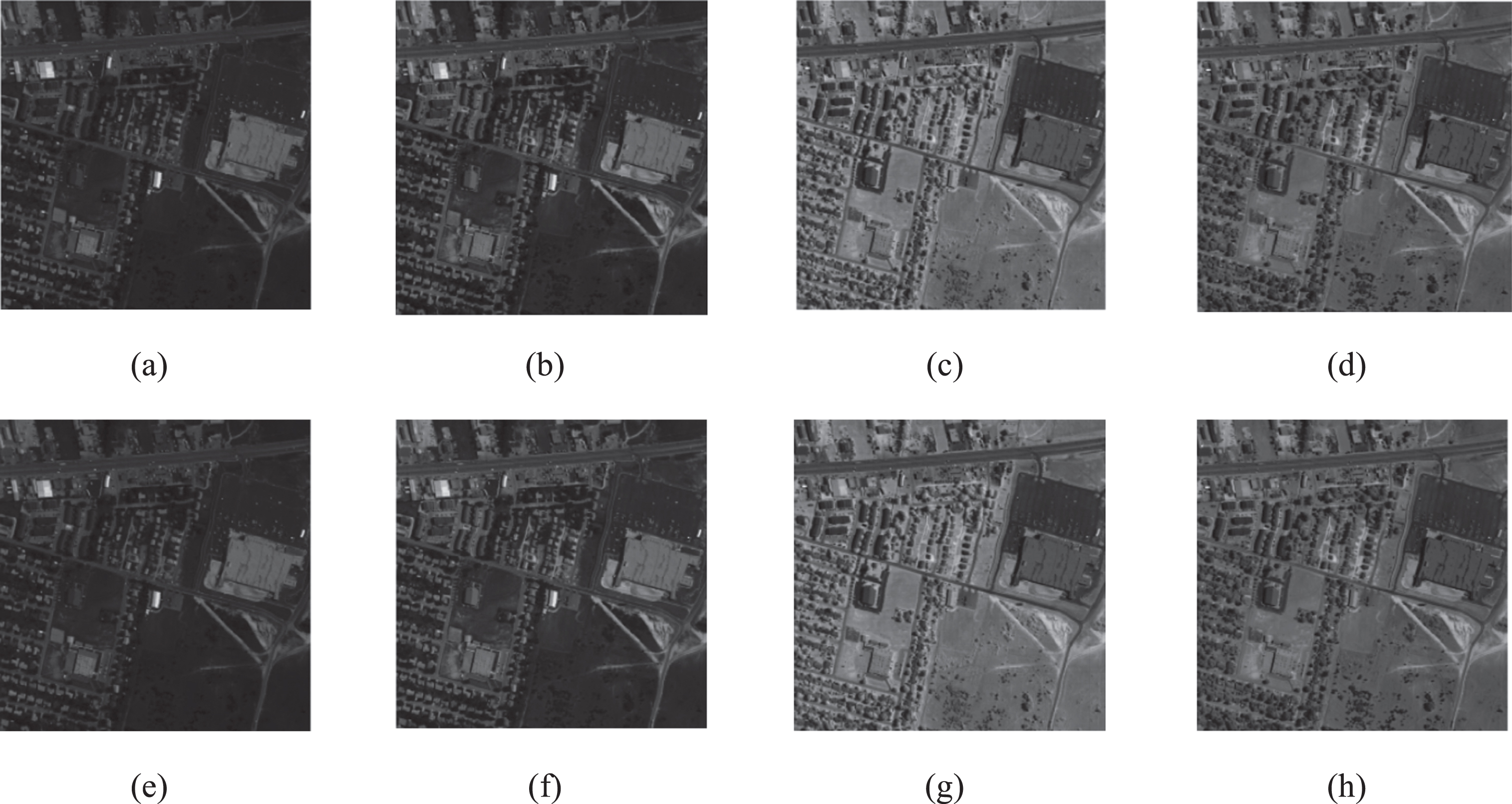
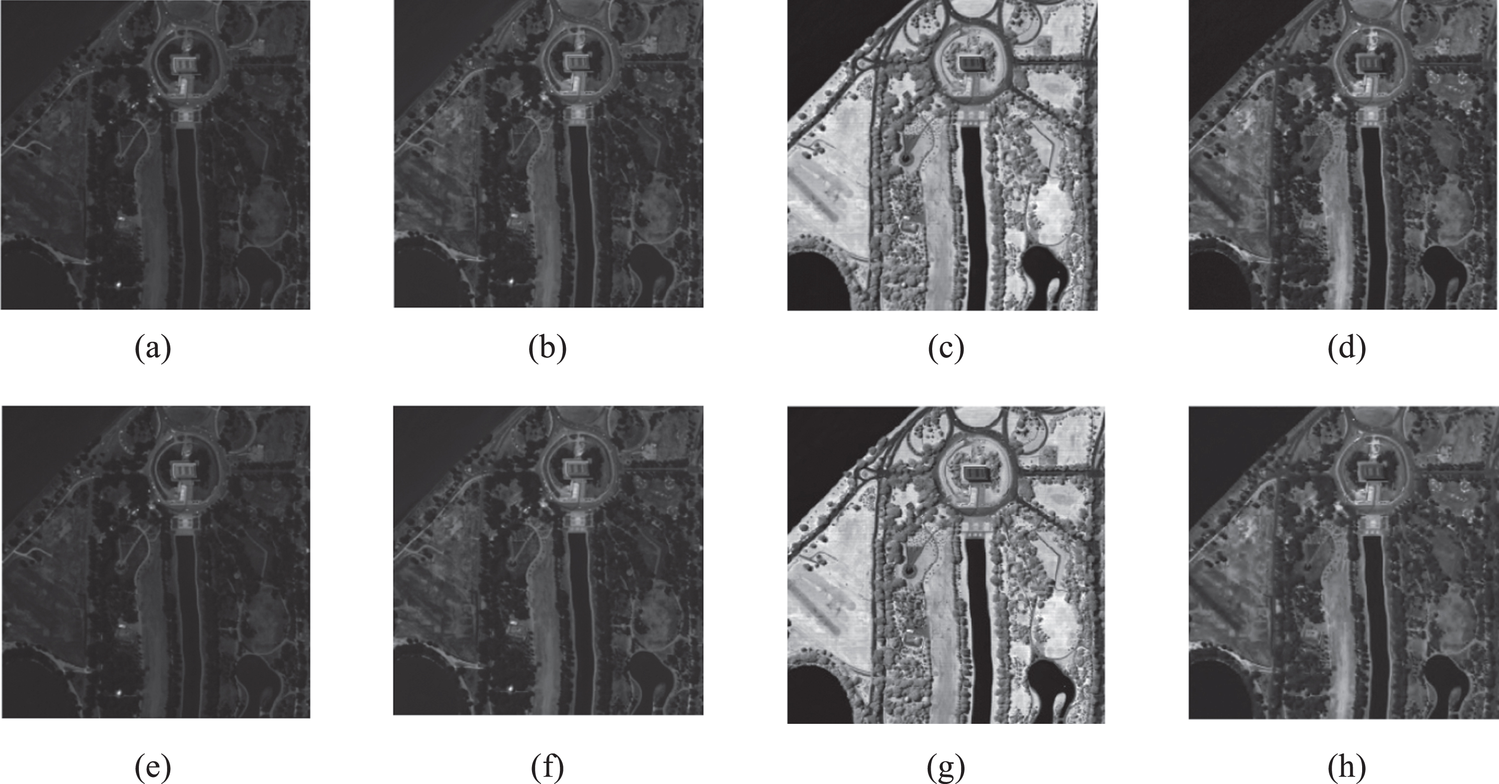
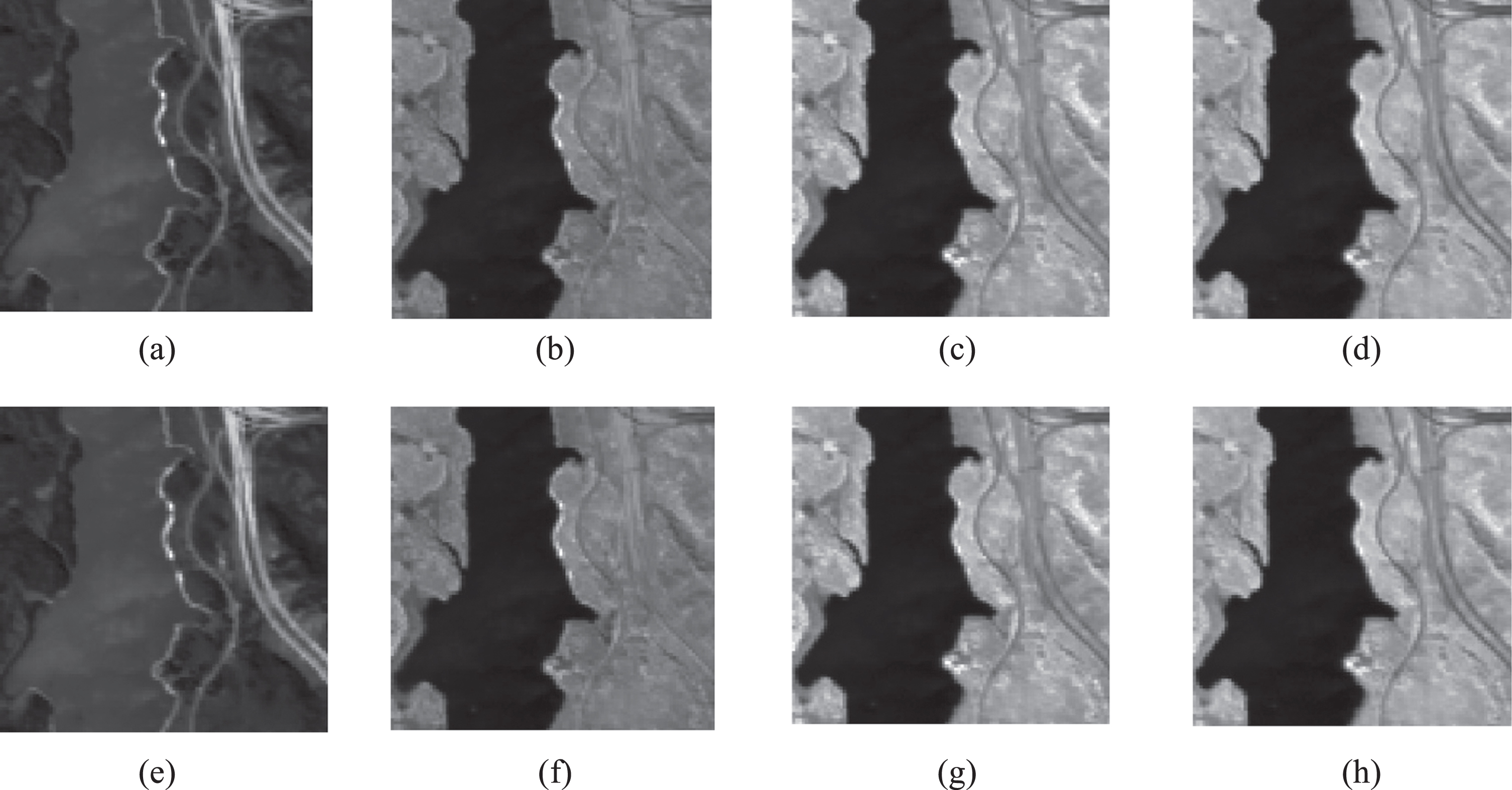
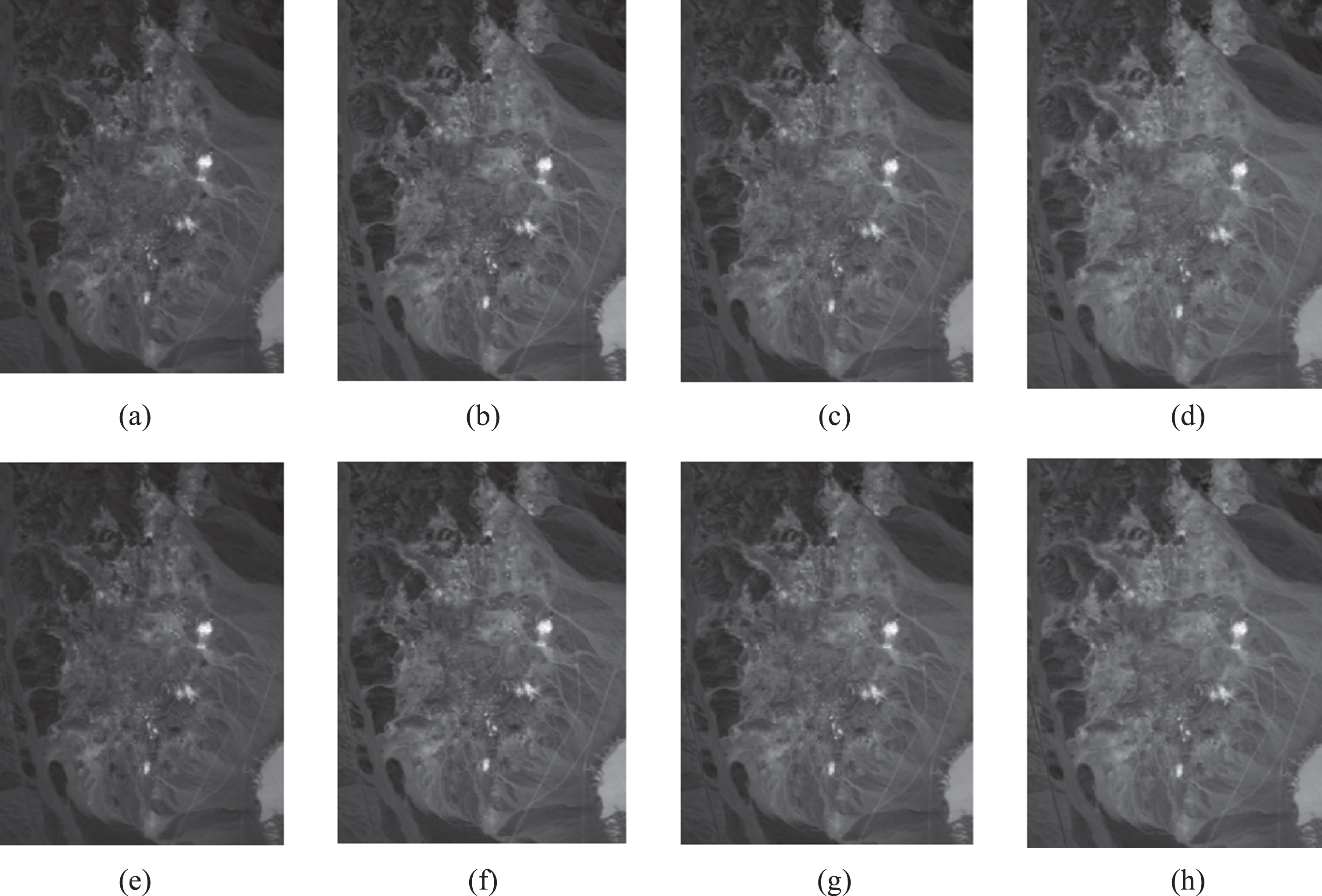
The visual representation of the HS images (before compression & after compression process) for the four sub bands (frame 30, 60, 90 & 120) of Urban HS image and Washington DC MALL HS image is shown in the Figs. 3. In the same way, visual illustration for the Cuprite and Jasper Ridge hyperspectral images for four different frequency frames (20, 40, 60 and 80) is covered in Figs. 5.

Fig. 2

Original Urban HS image (a) Frame 30 (b) Frame 60 (c) Frame 90 (d) Frame 150. Reconstructed Urban HS image with CR 10 (e) Frame 30 (f) Frame 60 (g) Frame 90 (h) Frame 150.

Fig. 3

Original Washington DC MALL HS image (a) Frame 30 (b) Frame 60 (c) Frame 90 (d) Frame 150. Reconstructed Washington DC MALL HS image with CR 14 (e) Frame 30 (f) Frame 60 (g) Frame 90 (h) Frame 150.

Fig. 4

Original Jasper Ridge HS image (a) Frame 20 (b) Frame 40 (c) Frame 60 (d) Frame 80. Reconstructed Jasper Ridge HS image with CR 13 (e) Frame 20 (f) Frame 40 (g) Frame 60 (h) Frame 80.

Fig. 5

Original Cuprite HS image (a) Frame 20 (b) Frame 40 (c) Frame 60 (d) Frame 80. Reconstructed Cuprite HS image with CR 16 (e) Frame 20 (f) Frame 40 (g) Frame 60 (h) Frame 80.

5 Conclusion

The onboard HS image sensor only has a limited amount of resources to use for processing and transmitting HS images to the earth station. In this research, a unique technique is proposed that outperforms conventional transform-based HS image compression algorithms that are currently considered state of the art in terms of coding efficiency and computational complexity. The coding gain has been increased across virtually the whole range of bit rates, and it has been demonstrated that the proposed 3D-MELS has a positive Bjontegaard Delta PSNR gain across all HS images.

The curvelet transform requires a lower number of coefficients in order to accurately represent the edges in the HS image, which results in an increase in the coding gain. When compared to other zerotree HSICAs, such as 3D-SPIHT and 3D-NLS, the coding memory consumption is greatly decreased. The intricacy of the computational complexity just a little bit increased. The low coding memory needs of 3D-MELS more than make up for the algorithm’s slightly higher level of complexity. The coding gain can be improved with the application of the bandlet and ripplet transforms. By utilizing a lower total number of markers, the load placed on coding memory can be decreased.

6 Declarations

Footnotes

Acknowledgments

We are sincerely thankful to the anonymous reviewers for their critical comments and suggestions to improve the quality of the paper. The authors want to express his gratitude to Integral University, Lucknow for providing manuscript number IU/R&D/2023-MCN0001906 for the present research work.

Authors’ contributions

Chandra developed the algorithm, algorithms simulation, prepare the manuscript, Bajpai supervised & Alam, Chandel, Panday and Pandey reviewed the manuscript.

Competing interests

The authors have declared that no competing interests exist.

Ethical approval

Not applicable

Consent for publication

All authors agreed on the final approval of the version to be published.

Funding

The authors receive no funding for the publication of the manuscript.

Data availability

Data is available within the manuscript.

References

Campbell

, Zabalza

, Murray

, Marshall

and Malone

, Hyperspectral imaging through partially transparent media, In Hyperspectral Imaging and Applications II 12338 (2023), 61–66. DOI: 10.1117/12.2653629

Mukundan

, Tsao

Y.M.

, Cheng

W.M.

, Lin

F.C.

and Wang

H.C.

, Automatic counterfeit currency detection using a novel snapshot hyperspectral imaging algorithm, Sensors 23(4) (2023), 2026. DOI: 10.3390/s23042026

Chandrasekaran

, Panigrahi

S.S.

, Ravikanth

and Singh

C.B.

, Potential of near-infrared (NIR) spectroscopy and hyperspectral imaging for quality and safety assessment of fruits: An overview, Food Analytical Methods 12 (2019), 2438–2458. DOI: 10.1007/s12161-019-01609-1

Banerjee

B.P.

, Raval

and Cullen

P.J.

, UAV-hyperspectral imaging of spectrally complex environments, International Journal of Remote Sensing 41(11) (2020), 4136–4159. DOI: 10.1080/01431161.2020.1714771

Bajpai

, Singh

H.V.

and Kidwai

N.R.

, Feature extraction and classification of hyperspectral images using singular spectrum analysis & multinomial logistic regression classifiers, In Proceedings on Multimedia, Signal Processing and Communication Technologies (IMPACT) Aligarh, India, 2017:97–100. DOI: 10.1109/MSPCT.2017.8363982

Chandra

and Bajpai

, Listless block cube tree coding for low resource hyperspectral image compression sensors, In 2022 5th International Conference on Multimedia, Signal Processing and Communication Technologies (IMPACT), 2022:1–5. DOI: 10.1109/IMPACT55510.2022.10029076

Dua

, Kumar

and Singh

R.S.

, Comprehensive review of hyperspectral image compression algorithms, Optical Engineering 59(9) (2020), 090902–090902. DOI: 10.1117/1.OE.59.9.090902

Dua

, Singh

R.S.

, Parwani

, Lunagariya

and Kumar

, Convolution neural network based lossy compression of hyperspectral images, Signal Processing: Image Communication 95 (2021), 116255. DOI: 10.1016/j.image.2021.116255

Dua

, Kumar

and Singh

R.S.

, Parallel lossless HSI compression based on RLS filter, Journal of Parallel and Distributed Computing 150 (2021), 60–68. DOI: 10.1016/j.jpdc,2020.12.004

10.

Bajpai

, Naimur

R.K.

and Vishal

S.C.

, Low memory wavelet based hyperspectral image coding using 2D Dyadic Wavelet Transform, International Journal of Electrical Engineering and Technology 11(6) (2020), 25–33. DOI: 10.34218/IJEET.11.6.2020.003

11.

Bajpai

, Sharma

, Alam

, Chandel

V.S.

, Pandey

A.K.

and Tripathi

S.L.

, Curvelet Transform Based Compression Algorithm for Low 659 Resource Hyperspectral Image Sensors, Journal of Electrical and Computer Engineering 2023:1–18. DOI: 10.1155/2023/8961271

12.

Valsesia

and Magli

, Fast and lightweight rate control for onboard predictive coding of hyperspectral images, IEEE Geoscience and Remote Sensing Letters 14(3) (2017), 394–398. DOI: 10.1109/LGRS.2016.2644726

13.

Wang

, Tao

, Shen

, Qin

and Song

, Distributed source coding of hyperspectral images based on three-dimensional wavelet, Journal of the Indian Society of Remote Sensing 46(4) (2018), 667–673. DOI: 10.1007/s12524-017-0735-1

14.

Gunasheela

K.S.

and Prasantha

H.S.

, Compressive sensing approach to satellite hyperspectral image compression, Information of Communication Technology for Intelligent Systems 2019. https://doi.org/10.1007/978-981-13-1742-2_49

15.

Das

, Hyperspectral image, video compression using sparse tucker tensor decomposition, IET Image Processing 15(4) (2021), 964–973. DOI: 10.1049/ipr2.12077

16.

Kumar

, Chaudhuri

, Banerjee

and Ali

, Onboard hyperspectral image compression using compressed sensing and deep learning, In Proceedings of the 2018 IEEE European conference on computer vision (ECCV), Munich, Germany, 2018; 30–42. doi :10.1007/978-3-030-11012-3_3

17.

Jiang

, Pan

W.D.

and Shen

, Spatially and spectrally concatenated neural networks for efficient lossless compression of hyperspectral imagery, Journal of Imaging 6(6) (2020), 38. doi: 10.3390/jimaging6060038

18.

Chandra

and Bajpai

, 3D-Block Partitioning Embedded Coding for Hyperspectral Image Sensors, International Conference on Power, Instrumentation, Energy, and Control (PIECON-2023), AMU Aligarh, India, 2023. doi: 10.1109/PIECON56912.2023.10085841

19.

Altamimi

and Ben

Y.B.

, A systematic review of hardware-accelerated compression of remotely sensed hyperspectral images, Sensors 22(1) (2022), 263. DOI: 10.3390/s22010263

20.

Tang

and Pearlman

W.A.

, Lossy-to-lossless block-based compression of hyperspectral volumetric data, IEEE International Conference on Image Processing, Singapore 5 (2004), 3283–3286. DOI: 10.1109/ICIP.2004.1421815

21.

Tang

and Pearlman

W.A.

, Three-dimensional wavelet-based compression of hyperspectral images, In Hyperspectral Data Compression Springer, Boston, MA. 2006; 273–308. DOI: 10.1007/0-387-28600-4_10

22.

Bajpai

, Harsh

V.S.

and Naimur

R.K.

, 3D Wavelet Block Tree Coding for Hyperspectral Images, International Journal of Innovative Technology and Exploring Engineering 8(6C) (2019), 64–68.

23.

Ngadiran

, Boussakta

, Sharif

and Bouridane

, Efficient implementation of 3D listless SPECK. IEEE international conference on computer and communication engineering, 2010; 1–4. DOI: 10.1109/ICCCE.2010.5556843

24.

Sudha

V.K.

and Sudhakar

, 3D listless embedded block coding algorithm for compression of volumetric medical images, Journal of Scientific and Industrial Research 72 (2013), 735–748.

25.

Bajpai

, Naimur

R.K.

, Harsh

V.S.

and Amit

K.S.

, Low memory block tree coding for hyperspectral images, Multimedia Tools and Applications 78(19) (2019), 27193–27209. DOI: 10.1007/s11042-019-07797-6

26.

Bajpai

, Naimur

R.K.

, Harsh

V.S.

and Amit

K.S.

, A low complexity hyperspectral image compression through 3D set partitioned embedded zero block coding, Multimedia Tools and Applications 81(1) (2022), 841–872. DOI: 10.1007/s11042-021-11456-0

27.

Bajpai

, Low complexity image coding technique for hyperspectral image sensors, Multimedia Tools and Applications 82(20) (2023), 31233–31258. DOI: 10.1007/s11042-023-14738-x

28.

Bajpai

, Low complexity block tree coding for hyperspectral image sensors, Multimedia Tools and Applications 81(23) (2022), 33205–33232. DOI: 10.1007/s11042-022-13057-x

29.

Hou

and Liu

, 3D set partitioned embedded zero block coding algorithm for hyperspectral image compression, Remote Sensing and GIS Data Processing and Applications; and Innovative Multispectral Technology and Applications 6790 (2007), 679056. DOI: 10.1117/12.750975

30.

Boettcher

J.B.

, Du

and Fowler

J.E.

, Hyperspectral image compression with the 3D dual-tree wavelet transform, IEEE International Geoscience and Remote Sensing Symposium 2007; 1033–1036. DOI: 10.1109/IGARSS.2007.4422977

31.

Taha

M.S.

, Rahem

M.S.M.

, Hashim

M.M.

and Khalid

H.N.

, High payload image steganography scheme with minimum distortion based on distinction grade value method, Multimedia Tools and Applications 81(18) (2022), 25913–25946. DOI: 10.1007/s11042-022-12691-9

32.

Inouri

, Tighidet

, Azni

, Khireddine

and Harrar

, A fast and efficient approach for image compression using curvelet transform, Sensing and Imaging 19 (2018), 1–23. DOI: 10.1007/s11220-018-0212-0

33.

Tong Qiao

, Jinchang

, Zheng

, Jaime

, Meijun

, Huimin

, Shutao

, Jón

A.B.

, Qingyun

and Stephen

, Effective denoising and classification of hyperspectral images using curvelet transform and singular spectrum analysis, IEEE Transactions on Geoscience and Remote Sensing 55(1) (2016), 119–133. DOI: 10.1109/TGRS.2016.2598065

34.

Saha

, Naskar

M.K.

and Chatterji

B.N.

, Advanced wavelet transform for image processing-a survey, In Information, Photonics and Communication: Proceedings of Second National Conference, IPC 2019. 2020; 185–194. DOI: 10.1007/978-981-32-9453-0_19

35.

Iqbal

M.A.

, Javed

M.Y.

and Qayyum

, Curvelet-based image compression with SPIHT, In 2007 International Conference on Convergence Information Technology (ICCIT 2007), 2007; 961–965. DOI: 10.1109/ICCIT.2007.280

36.

Setiadi

D.R.I.M.

, PSNR vs SSIM: imperceptibility quality assessment for image steganography, Multimedia Tools and Applications 80(6) (2021), 8423–8444. DOI: 10.1007/s11042-020-10035-z

37.

Sara

, Akter

and Uddin

M.S.

, Image quality assessment through FSIM, SSIM, MSE and PSNR—a comparative study, Journal of Computer and Communications 7(3) (2019), 8–18. DOI: 10.4236/jcc.2019.73002

38.

Barman

, Martini

M.G.

and Reznik

, Revisiting Bjontegaard delta bitrate (BD-BR) computation for codec compression efficiency comparison, In Proceedings of the 1st Mile-High Video Conference, 2022; 113–114. 10.1145/3510450.3517289

39.

Soccio

, Barbosa

J.P.

and Reis

M.S.

, A scalable approach for the efficient segmentation of hyperspectral images, Chemometrics and Intelligent Laboratory Systems 213 (2021), 104314. DOI: 10.1016/j.chemolab.2021.104314

40.

Kidwai

N.R.

, Khan

and Reisslein

, ZM-SPECK: A fast and memoryless image coder for multimedia sensor networks, IEEE Sensors Journal 16(8) (2016), 2575–2587. DOI: 10.1109/JSEN.2016.2519600

41.

Tausif

, Kidwai

N.R.

, Khan

and Reisslein

, FrWF-based LMBTC: Memory-efficient image coding for visual sensors, IEEE Sensors Journal 15(11) (2015), 6218–6228. DOI: 10.1109/JSEN.2015.2456332

42.

Bajpai

, Low Complexity and Low Memory Compression Algorithm for Hyperspectral Image Sensors, Wireless Personal Communications 131(2) (2023), 805–833. DOI: 10.1007/s11277-023-10455-8

3D-Memory efficient listless set partitioning in hierarchical trees for hyperspectral image sensors

Abstract

Keywords

1 Introduction

2 Related work

2.1 3D set partitioned transform based HS image compression algorithms

3 Proposed 3D memory efficient listless SPIHT (3D-MELS)

3.1 Initialization pass (IP)

3.2 Bit plane pass (BPP)

Table 4 Description of HS images used for the experiment HS image HS image Spatial Spectral Pixel dataset sensor dimension dimension depth Washington DC Mall HYDICE 1280 × 307 191 14 Urban 307 × 307 210 10 Jasper Ridge AVIRIS 100 × 100 224 13 Cuprite 250 × 190 224 16

6 Declarations

Footnotes

Acknowledgments

Authors’ contributions

Competing interests

Ethical approval

Consent for publication

Funding

Data availability

References

Table 4
Description of HS images used for the experiment

HS image HS image Spatial Spectral Pixel

dataset sensor dimension dimension depth

Washington DC Mall HYDICE 1280 × 307 191 14

Urban 307 × 307 210 10

Jasper Ridge AVIRIS 100 × 100 224 13

Cuprite 250 × 190 224 16