Anomaly detection for high-dimensional data using a novel autoencoder-support vector machine

Abstract

Aiming at anomaly detection upon a high-dimensional space, this paper proposed a novel autoencoder-support vector machine. The key thought is that using the autoencoder extracts the features from high-dimensional data, and then the support vector machine achieves the separation of abnormal features and normal features. To increase the precision of identifying anomalies, Chebyshev’s theorem was used to estimate the upper of the number of abnormal features. Meanwhile, the dot product operation was implemented in order to strengthen the learning of the model for class labels. Experiment results show that the detected accuracy of the proposed method is 0.766 when the data dimensionality is 5408, and also wins over competitors in detected performance for the considered cases. We also demonstrate that the strengthened learning of class labels can improve the ability of the model to detect anomalies. In terms of noise resistance and overcoming the curse of dimensionality, the former can carry out more efforts than the latter.

Keywords

Anomaly detection Chebyshev’s theorem high-dimensional data

1 Introduction

Usually, anomaly detection is treated as sample identification that does not confirm to the regular patterns or the expected distribution of normal samples [1]. Anomaly detection has been applied in many fields, such as, video surveillance [2, 3], remote sensing [4, 5], and medical diagnosis [6]. Usually, real-world data, e.g., ecological data, economic data, is high dimensionality. Due to high dimensionally of the data, i.e., the so-called the curse of dimensionality, there suffers troubles form mining anomalies, for instance, (i) anomalies easily show anomalous features in a low-dimensional space, instead, those anomalous features become hidden in a high-dimensional space. Most existing detection methods implicitly or explicitly rely on the measurement of the distance between the data, unfortunately, the relative contrast of the distance drops as the dimensionality of the data increases [7 –9]. (ii) Anomalies can exist in any of subspaces of a high-dimensional space, because of the rare characteristic of anomalies, anomaly labels are difficult collected in exponential search space.

Some efforts have devoted into the anomaly detection, including deep feature representations-based -based methods, e.g., these methods implemented in [10, 11] gain the superior detection results. Such methods are very good at handling the high dimensionality of the data, since they contain several layers of nonlinear processing nodes to capture the low-dimensional representations of high-dimensional data. And classification-based methods, which do not have to pretreat the data before training the model, e.g., One Class-Support Vector Machine (OC-SVM) [12]. Additionally, Khalid [13 –16] et al. proposed the method. From the algorithm level point of view, distance measurement-based methods, reconstructed error-based methods and classification-based methods do not have to pretreat data distributions [17]. From the data level of perspective, deep feature representations-based methods, deep hybrid-based methods can capture the feature representations of the data, which effectively reduce the complex of the search space providing for anomaly detection.

1.1 Distance measurement-based methods

Such methods include B-KNN (k-nearest neighbor) [18], KNN [19], etc. Guansong [20] et al. and Hu [21] et al. utilized the random distance in dealing with anomaly detection. They gain better performance in the case of a few number of anomalies [22], and do not specify data distribution assumptions. But unfortunately, they perform not well in handling ‘the curse of dimensionality’, and suffer from failing in high-dimensional noise environment [23]. To improve the detection accuracy, Mao et al. [24] proposed an anomalous method through assessing the changes in angle of data objects, instead of the assessment of the distance between the data.

1.2 Reconstructed error-based methods

Points with reconstruction error greater than the preset threshold are considered as anomalies in this strategy. Detected accuracy of such methods relies on the reconstructed errors, such as, Principal Components Analysis (PCA) [25, 26]. Although PCA has outstanding ascendancy in calculating speed and cost, it cannot get good results for nonlinear dependence because of linearly calculated manner. To address this, X. He [27] et al. proposed the fast matrix factorization (MF) for nonlinear dependence. Similarly, the MF in [28] and [29]. MF methods make up the gap of PCA methods, nevertheless, they still have weak capabilities to resist the curse of dimensionality.

1.3 Classification-based methods

Classification-based methods are good at projecting high-dimensional data onto a lower-dimensional space so that they work on a simpler data space well [30]. This is beneficial for revealing those hidden anomalies on the projected lower-dimensional space, e.g., the OC-SVM [31 –33]. However, such methods may not retain sufficient information for anomaly detection because of fully decoupling during the data projection. Anomalies themselves can provide very little information, once they are completely decoupled, the information may be fully lost.

1.4 Deep feature representations-based methods

Deep feature representations-based methods can overcome the curse of dimensionality because of extracting the low dimensional representations of the data, e.g., these methods implemented in [34] and [35], and Deep One-class Classification (DOC) [36]. Auto encoder (AE) are also usually used for anomaly detection, e.g., Sparse AE (SAE) [37], Motion United-AE [38] and Deep Graph Auto-encoder [39]. Due to the design of the loss functions aims at feature extraction, AE is more suitable for data compression or dimension reduction [40].

1.5 Deep hybrid-based methods

This type of methods consists of deep network architectures and traditional methods, e.g., Deep Neural Networks-Support Vector Machine (DNN-SVM) [41], deep autoencoder and ensemble k-nearest neighbor (DAE-KNN) [42], and deep autoencoder model combining with hypersphere (DM-HS) [23]. Sangwook [43] et al. proposed K-DNN-SVM method, which utilized the support vector machine (SVM) to judge anomalies in the feature space reconstructed by the K-classification deep neural networks. The detection ability of K-DNN-SVM depends on data volume, when data points are rarity, the quality of the reconstructed feature space is deteriorated. Usually, the deeper the hybrid model is, the better the performance it gains [44]. By contrary, the deeper network architectures need to afford dear cost of tuning parameters and time consuming. Overall, deep hybrid-based methods show natural advantages in addressing anomaly detection for high-dimensional data since they inherit the advantages of deep network architectures and traditional methods.

Beyond that, support vector machine (SVM)-based architectures are also used for anomaly detection, e.g., Sparse SVM [45], the SVM [46]. SVM-based architectures can gain superior detected results on the low-dimensional data, while they easily suffer the limitation of linear inseparability on the high-dimensional data, since the features obtained are quite limited for building the proper classification boundaries [23]. From the point view of structures, shallow structures being similar to SVMs are failure to extract the dependencies between variables [47]. SVMs can take advantages in anomaly detection once there provide favorable low-dimensional space environments for them.

1.6 Motivations

The motivation of this work is to mine a limited number of potential anomaly instances upon a high-dimensional space, and to provide the insights for anomaly detection. Additionally, to propose some measures in improving detection precision, we also discussed the relative importance of the effect indicators noise and data dimensionality. Given that these complementary advantages between auto encoders and SVMs, this is very valuable to develop the hybrid model of both aiming at anomaly detection on high-dimensional data. The hybrid model not only better captures robust features from the input data, but also has the ability of distinguishing the potential anomalies. Hence, this paper proposes a novel autoencoder-support vector machine. Using the autoencoder extracts the features from high-dimensional data, then the support vector machine achieves the separation of abnormal features and normal features. To increase the precision of anomaly detection, using Chebyshev’s theorem estimates the upper of abnormal feature quantity. Furthermore, the dot product operation is also implemented to strengthen the learning of the model for class labels.

1.7 Contribution

We summarize main contributions of this work, as follows

The proposed model resists the curse of dimensionality to a certain extent since the dot product operation strengthens the ability to learn the class labels.

Noise has more negative effects on anomaly detection accuracy than data dimensionality does, so that the former can carry out more efforts than the latter in improving detection accuracies.

The rest of this paper is organized as follows. The proposed method is illustrated in Section 2. The experimental details are illustrated in Section 3. Section 4 exhibits experimental results and the discussion. Section 5 draws a conclusion.

2 Methodology

2.1 Background

Raghavendra [48] et al. define that anomaly is defined as an observation that deviates so significantly from other observations as to arouse suspicion from the view of data distribution. Figure 1 visualizes the definition of high-dimensional anomalies that are projected onto 2-dimensional space, where point P1 and point P2 and these points in the region R2 are defined anomaly instances. These points in the region R1 are regarded as normal instances.

Fig. 1

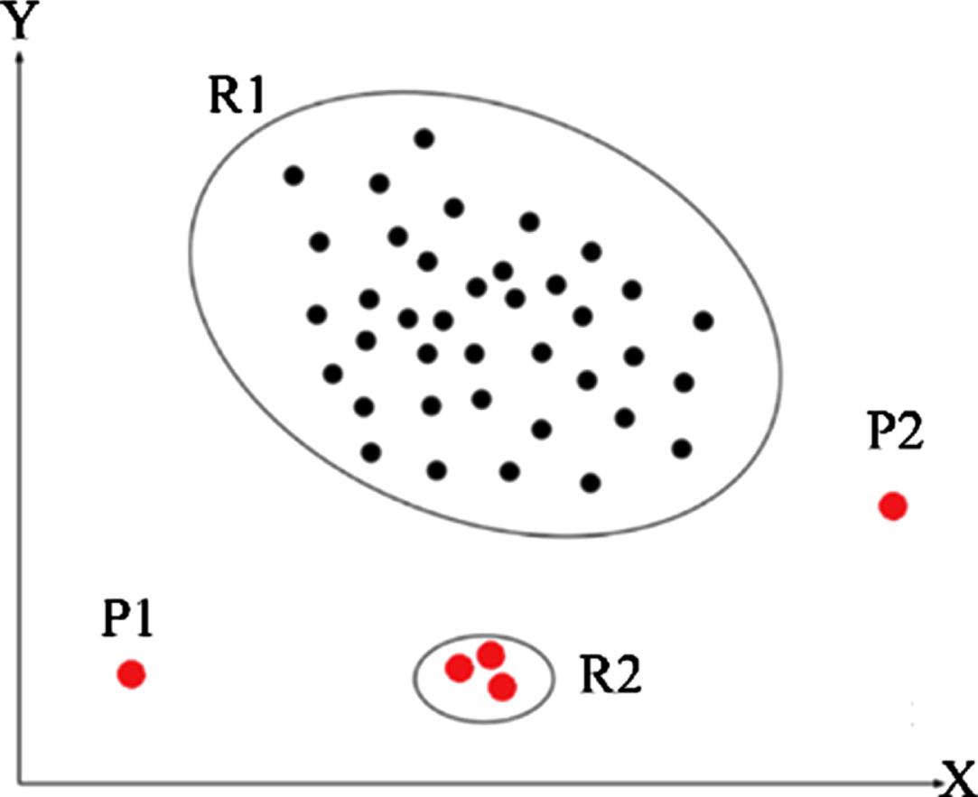
Definition of anomalies. It is cited by the [1]. Red circles are regarded as anomaly instances. Black circles are normal instances.

Pang [49] et al. define that anomaly detection is regarded as the procedure of detecting data instances that significantly deviate from the majority of data instances. Similarly, we give the definition of anomaly detection in this work. The details of symbols are interpreted in Appendix Table 3.

Definition 1. Abnormal detection. Given h-dimensional dataset $X = {x_{i}, i = 1, 2, . . .}^{h} \in R^{D}$ , x_i is the data point. $Y = {y_{j}, j = 1, 2, . . .}^{l} \in R^{l}$ is the corresponding feature space of X, where y_j is the low-dimensional feature. Abnormal detection is to train a model by using X, and to strengthen that the model learns class labels. Class labels consist of normal class label +1 and abnormal class label -1. The model outputs the learned class labels C = {+1, . . . +1, . . . , -1, . . . , -1}.

Lemma 1 [50]. Mercer theorem indicates that any semi-positive definite symmetric function can be allowed to be used as a kernel function.

Lemma 2 [51]. Let χ be a nonempty set. A kernel $κ : (χ \times χ) \to R$ is called a positive definite kernel if κ is symmetric and $\sum_{i, j = 1}^{n} c_{i} c_{j} κ (x_{i}, x_{j}) ⩾ 0$ for all on n ∈ N, {χ₁, . . . , χ_n} ∈ χ and ${c_{1}, . . ., c_{n}} \in R$ .

Lemma 3 [52]. Chebyshev’s theorem. For any set of observations (sample or population), the proportion of the values that lie within m standard deviations of the mean is $P (| X - \bar{u} | ⩾ λ σ) ⩽ 1 / λ^{2}$ , where $\bar{u}$ , σ are the data mean and the standard deviation of the data, respectively. λ is the number of standard deviations from the mean.

2.2 The scheme

The scheme contains feature extraction stage, feature separation stage and class label output stage. Because complex high-dimensional space is not beneficial for the searching of anomalies, using the encoder extracts the low-dimensional features from X in feature extraction stage. By doing so, favorable space environments can be created for anomaly detection. Utilizing the SVM separates anomaly and normal features in feature separation stage. And the number of anomaly features are estimated by the Chebyshev’s theorem to promote the separated precision. Finally, the decoder sends out the learned class labels in class label output stage. The details are as follows.

(1) Feature extraction

The autoencoder with multiple hidden layers is designed to extract features, illustrated in Fig. 2. The error e_PO between the prediction and the output is obtained, and the label vector V_label is generated according to the prediction results. Thereafter, e_PO and V_label implement the dot product operation, where ⊗ represents the dot product operation. The results of the dot product are added the loss function. The label vector V_label is to strengthen the model to learn normal class labels. If the predicted result is normal, there generates a normal class label +1, and let V_label = [1]. Similarly, if the predicted result is anomaly, there generates an abnormal class label -1, and let V_label = [0]. Label vector V_label is a unit vector consisting of zero and 1. Eq. (1) gives the loss function L_function of the autoencoder.

Fig. 2

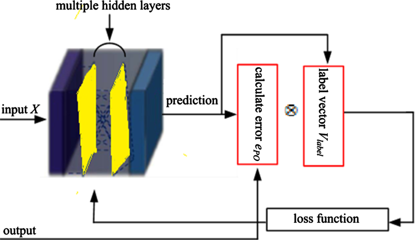
The autoencoder. It has multiple hidden layers, and the dot product operation is introduced.

$L_{function} = \sum (x_{i} - {\hat{x}}_{i})^{2}$ (1) ${\hat{x}}_{i} = ζ (w • (x_{i} \otimes V_{label}) + b)$ (2)

Where ζ is an activation function. w, b are the weight and the bias, respectively. x_i, ${\hat{x}}_{i}$ are the input and corresponding reconstructed input, respectively.

(2) Feature separation

Normal features and abnormal features can be separated in the extracted features, due to the difference between the both, the SVM can separate them. The SVM can be given as follows $\begin{matrix} min_{w, b, ξ} (\frac{1}{2} | | w | |^{2} + θ ξ) \\ s . t . c_{i} (w^{T} y_{i} + b) ⩾ 1 - ξ, i = 1, 2, . . ., \\ ξ ⩾ 0 \end{matrix}$ (3)

Where ξ is a slack variable. θ > 0 is just a penalty item and is not a training parameter. y_i is the feature in definition 1. c_i is the corresponding label of y_i. w is the weight vector.

Using Lagrange function [53] covert Eq. (3) into Eq. (4) according to KKT (Karush-Kuhn-Tucker) [53]. As follows $f = \sum y_{i} α_{i} κ + b$ (4)

Where α_i > 0 is the Lagrange multiplier. κ is a positive definite (p.d. in Lemma2) kernel function satisfying the Mercer theorem (i.e., Lemma 1). The [53] gives the derived procedure.

The Matern52 kernel [54] is use as the kernel of the SVM, since it can make the radius to be warping concave and non-decreasing [54, 55], more areas with small radii can be observed. $\begin{matrix} κ = r_{1} (1 + \sqrt{A_{1} r_{2}^{2} (y_{1}, y_{2})} + A_{2} r_{2}^{2} (y_{1}, y_{2})) \\ exp {- \sqrt{A_{3} r_{2}^{2} (y_{1}, y_{2})}} [54] \end{matrix}$ (5)

Where r₁, r₂ are the kernel parameter and kernel radius, respectively. A₁, A₂, A₃ are constants.

(3) Abnormal feature estimation

The Chebyshev’s theorem, i.e., Lemma 3, estimates the number of abnormal features because of determining the upper regarding the percentage of the data that exists within λ number of standard deviations from the mean [52]. That is, the Chebyshev’s theorem can estimate that the percentage of abnormal feature quantity is lower than 1/λ² [52]. Hence, let parameter θ in Eq. (3) be not greater than 1/λ², that is, Eq. (3) is converted into Eq. (6), as follows $\begin{matrix} min_{w, b, ξ} (\frac{1}{2} | | w | |^{2} + \frac{1}{λ^{2}} ξ) \\ s . t . c_{i} (w^{T} y_{i} + b) ⩾ 1 - ξ, i = 1, 2, . . ., \\ ξ ⩾ 0 \end{matrix}$ (6)

2.3 Model implementation

Figure 3 displays the architecture of the model, which consists of the encoder module, the SVM module and the decoder module. The encoder module is used to extract the features from the input data, which corresponds to the feature extraction stage in Section 3.2. Using the SVM module separates abnormal features from normal features, corresponding to the feature separation stage. The decoder module sends out the learned class labels, similarly, this corresponds to the class label output stage.

Fig. 3

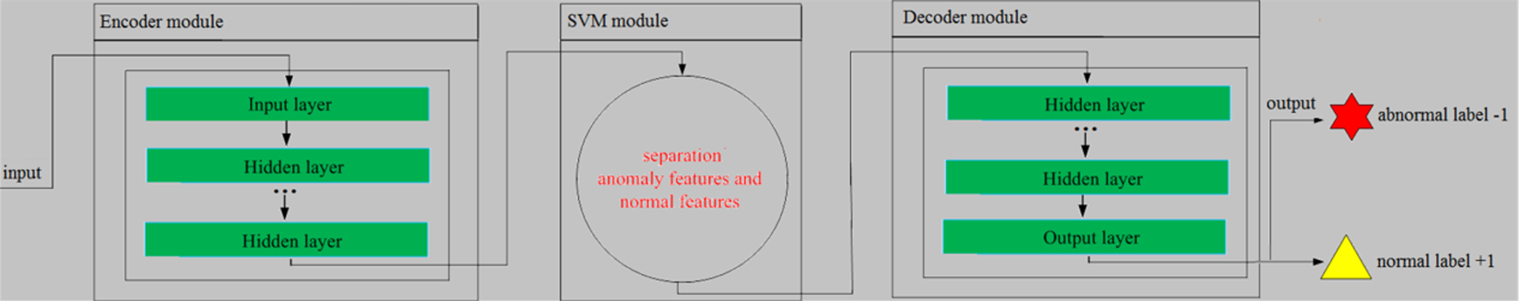
The architecture of the model. Encoder module and decoder module contain multiple hidden-layers, respectively.

Since the proposed model consists of the autoencoder and the SVM, namely AESVM, the objective function O (L_function, f) of AESVM contains the loss function L_function of the autoencoder in Eq. (1) and the function f of SVM in Eq. (4), having that $O (L_{function}, f) = L_{function} + f$ (7)

Algorithm 1 displays the training of AESVM. The benchmark dataset is divided into training set B^train and validation set B^val in step 1. The optimal parameter values is obtained in the procedure of step 2 to step 16, where the optimal hidden-layer quantity ϒ_Opt is obtained in the procedure of step 4 and step 12. Similarly, the optimal neuron quantity Π_Opt is obtained in step 3 to step 15. After gaining the optimal parameter values, using training dataset TrainingSet trains AESVM, illustrated in step 17 to step 22. Through iteratively learning the objective function O (L_function, f), the hyper parameters are updated. Then, the training is terminated until the hyper parameters can converge. Once AESVM is trained well, training accuracy TrainingAcc and class label C are sent out.

Algorithm 1. Training of AESVM.

Input: iteration epoch I, training set TrainingSet, benchmark set BenchmarkSet.

Output: training accuracy TrainingAcc, class label C = {+1, . . . +1, . . . , -1, . . . , -1}.

Begin:

1 Benchmark Dataset is divided into B^train, B^val;

2 fori = 1 toIdo:

3 foreachΠin {10, 30, 50, 70, 90, 100, 150, 200} do:

4. foreachϒin {1, 2, 3, 4, 5, 7, 10, 20, 30} do:

4 Use data set B^train to train AESVM;

5 Learn objective function O (L_function, f);

6 Update hyper parameters until they converge;

7 Calculate training accuracy;

8 Use data set B^val to verify AESVM;

9 Calculate validation accuracy;

10 end foreach

11 Select ϒ so that max(ϒ) = arg max(trainingaccuracy);

12 Obtain the optimal value ϒ_Opt = max(ϒ) of

hidden-layer quantity

13 end foreach

14 Select Π so that max(Π) = arg max(trainingaccuracy);

15 Obtain the optimal value of neuron quantity

Π_Opt = max(Π);

16 end for

17 fori = 1 toTdo:

18 Use training set TrainingSet to train

AESVM (Π_Opt, ϒ_Opt);

19 Learn objective function O (L_function, f);

20 Update hyper parameters until they converge;

21 Calculate training accuracy TrainingAcc;

22 end for

23 Select the i so that i_max = arg max(TrainingAcc);

24 Obtain maximum training accuracy in i_max-th iteration TrainingAcc = arg max(TrainingAcc);

25 Obtain class label C = {+1, . . . +1, . . . , -1, . . . , -1};

26 Output training accuracy TrainingAcc;

27 Output class label C;

End

3 Experiment settings

3.1 Datasets

Ten high-dimensional UCI (University of California Irvine) datasets were selected from different data dimensions, including two benchmark datasets B1, B2 and eight validation datasets U1-U8, as shown in Table 1. Benchmark datasets B1 and B2 are used to test parameters of AESVM. Datasets U1-U8 are used to verify AESVM and competitors. The ten datasets were pretreated by the manner in [56].

Table 1
Details of ten UCI datasets

Description Number of Anomaly Data

(Normal vs. Anomaly) Normal Anomaly Ratio Dimension

B1 SpamBase Spam vs. Non-spam 2528 1679 39.1% 57

B2 Hepatitis Survival vs. fatal 80 13 13.98% 19

U1 Musk musk vs non-musk 79699 269 0.34% 168

U2 APS negative vs. positive 59000 1000 1.67% 170

U3 HAR walking vs. Others 2830 30 1.05% 561

U4 CNAE zero vs non-zero values 918537 7023 0.76% 857

U5 Malware zero vs non-zero values 2894954 37772 1.29% 1087

U6 Micro Mass zero vs non-zero values 464819 3181 0.68% 1300

U7 InternetAds Ads vs. other images 3264 454 12.21% 1555

U8 p53Mutant inactive vs. active 16449 143 0.86% 5408

		Description	Number of	Anomaly	Data
B1	SpamBase	Spam vs. Non-spam	2528	1679	39.1%	57
B2	Hepatitis	Survival vs. fatal	80	13	13.98%	19
U1	Musk	musk vs non-musk	79699	269	0.34%	168
U2	APS	negative vs. positive	59000	1000	1.67%	170
U3	HAR	walking vs. Others	2830	30	1.05%	561
U4	CNAE	zero vs non-zero values	918537	7023	0.76%	857
U5	Malware	zero vs non-zero values	2894954	37772	1.29%	1087
U6	Micro Mass	zero vs non-zero values	464819	3181	0.68%	1300
U7	InternetAds	Ads vs. other images	3264	454	12.21%	1555
U8	p53Mutant	inactive vs. active	16449	143	0.86%	5408

We also generated 5 high-dimensional datasets without noise, denoted S1-S5, and 5 low-dimensional datasets containing noise, namely N1-N5. The ten synthetic datasets are used for verify the effects of noise and data dimensionality on detection performance, illustrated in Table 2. For the ten UCI and the ten synthetic datasets, the 70% of them were used for the training of our model, and the rest 30% were used for testing of our model.

Table 2

Details of ten synthetic datasets

	Description	Noise ratio	Number of		Anomaly	Data
	(Normal vs. Anomaly)		Normal	Anomaly	Ratio	Dimension
S1	1 vs 0	0%	5000	50	1%	100
S2	1 vs 0	0%	5000	50	1%	200
S3	1 vs 0	0%	5000	50	1%	300
S4	1 vs 0	0%	5000	50	1%	400
S5	1 vs 0	0%	5000	50	1%	500
N1	1 vs 0	10%	5000	50	1%	2
N2	1 vs 0	30%	5000	50	1%	2
N3	1 vs 0	50%	5000	50	1%	2
N4	1 vs 0	70%	5000	50	1%	2
N5	1 vs 0	90%	5000	50	1%	2

3.2 Competitors and parameters

Based on the architecture of AESVM, these competitors were considered, including deep hybrid-based methods DNN-SVM [41] and DAE-KNN [42], distance measurement-based method B-KNN [18], reconstructed error-based method MF [27], classification-based method OC-SVM [31], deep feature representations-based method SAE [37]. In addition, to verify the effort of the proposed dot product operation, we also designed a benchmark model referring to AESVM, namely BM-AESVM. Noting that benchmark model BM-AESVM has the same architecture and parameter configurations as AESVM, but without importing dot product operation.

We carefully studied AESVM parameters of having effects on learning results. Sigmoid function is used as the activation function of AESVM. Since the output of Sigmoid is just zero or 1, it is more suitable for the judgment of abnormal and normal instances. Studies indicate that neuron quantity is hard to be determined by experience [57]. Hence, the number of neuron Π ∈ {10, 30, 50, 70, 90, 100, 150} is determined within a certain range through validation testing. Similarly, the number of hidden-layer ϒ = {1, 2, 3, 4, 5, 7, 10, 20, 30} is determined within a certain range through validation testing. For the six competitors, we utilized the parameters provided by the corresponding literature.

3.3 Assessment metrics

Accuracy metric, F1-score metric and G-score metric are used as the evaluated indicators. $Accuracy = \frac{TP + TN}{TP + FP + TN + FN}$ (8) $F 1 - score = \frac{2 TP}{2 TP + FP + FN}$ (9) $G - score = \frac{TP}{TP + FN} \times \frac{TN}{FP + TN}$ (10)

Where TP, TN are the proportion of correctly predicted anomaly instances and correctly predicted normal instances, respectively. FP, FN are the proportion of incorrectly predicted anomaly instances and incorrectly predicted normal instances, respectively.

3.4 Experimental design and configurations

Experiment I. Parameter testing. To test parameters Π, ϒ of AESVM and BM-AESVM, the two models were run on benchmark datasets B1 and B2. Then, the run results were analyzed.

Experiment II. Ability comparisons of anomaly detection. To compare AESVM with competitors, they were run on validation datasets U1-U8, and the results were observed.

Experiment III. Affected indicators of detection accuracy. To analyze the effect factors noise and data dimensionality, the AESVM and the competitors were run on the ten synthetic datasets S1-S5 and N1-N5, and then we observe the results.

Ablation experiment. To verify the effort that the proposed dot product operation strengthens the learning of the model to class labels. In Experiment II, the ablation was supplemented.

The corresponding algorithms of these models are developed by using Python 3.8 in Tensorflow 2.0 of Linux operating system, then they were run on the Server with Intel i5 3.4 GHz CPU, 32 G memory.

4 Results and discussion

4.1 Parameter testing

Figure 4 unveils the testing results of the parameters, showing that our model AESVM and the benchmark model BM-AESVM obtain the best performance values in metrics Accuracy, F1-score and G-score when the number of neurons Π is equal to 50, and that of hidden layers ϒ is equal to 4. In Fig. 4(a), as the number of neurons start to increase from 10 to 50, the performance both AESVM and BM-AESVM augment. Once the values of neuron scale exceed 50, the two models decline in detected performance, this is because they happened over-fitting. Similarly, in Fig. 4(b), the number of hidden layers reach 4, the optimal performance is obtained for the two models. These demonstrate that the performance of AESVM and BM-AESVM gains the optimization when Π and ϒ reaches a certain scale on all considered case. Consequently, let Π, ϒ be equal to 50 and 4 in subsequent experiments, respectively.

Fig. 4

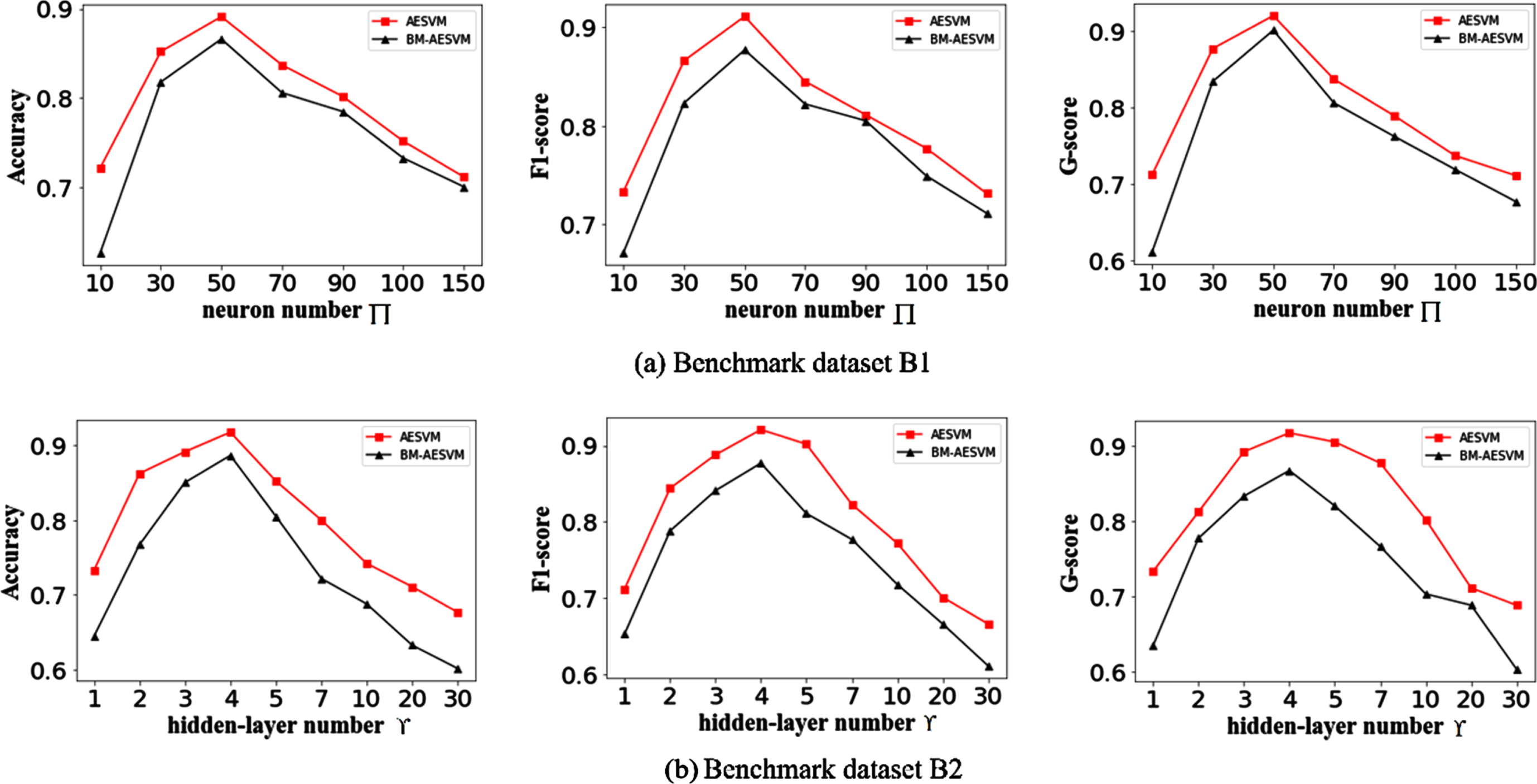
Results of parameter testing on benchmark datasets. (a) displays the testing of neural neuron quantity on dataset B1. (b) displays the testing of hidden-layer scale on dataset B2.

4.2 Comparisons of detected capabilities

Results in Fig. 5 show that AESVM outperforms four competing models on most datasets, e.g., U3-U8. Especially, on dataset U8 (dimension = 5408, anomaly ratio = 0.86%), AESVM has outstanding advantages over the competitors. This means that AESVM suffers less negative effects caused by the curse of dimensionality in handling anomaly detection for high-dimensional data. These detection results obtained by distance-based measurement, e.g., B-KNN and MF, are not as good as the other competitors on most datasets, which mean that distance-based measurement is not suitable for the anomaly detection for high-dimensional data.

Fig. 5

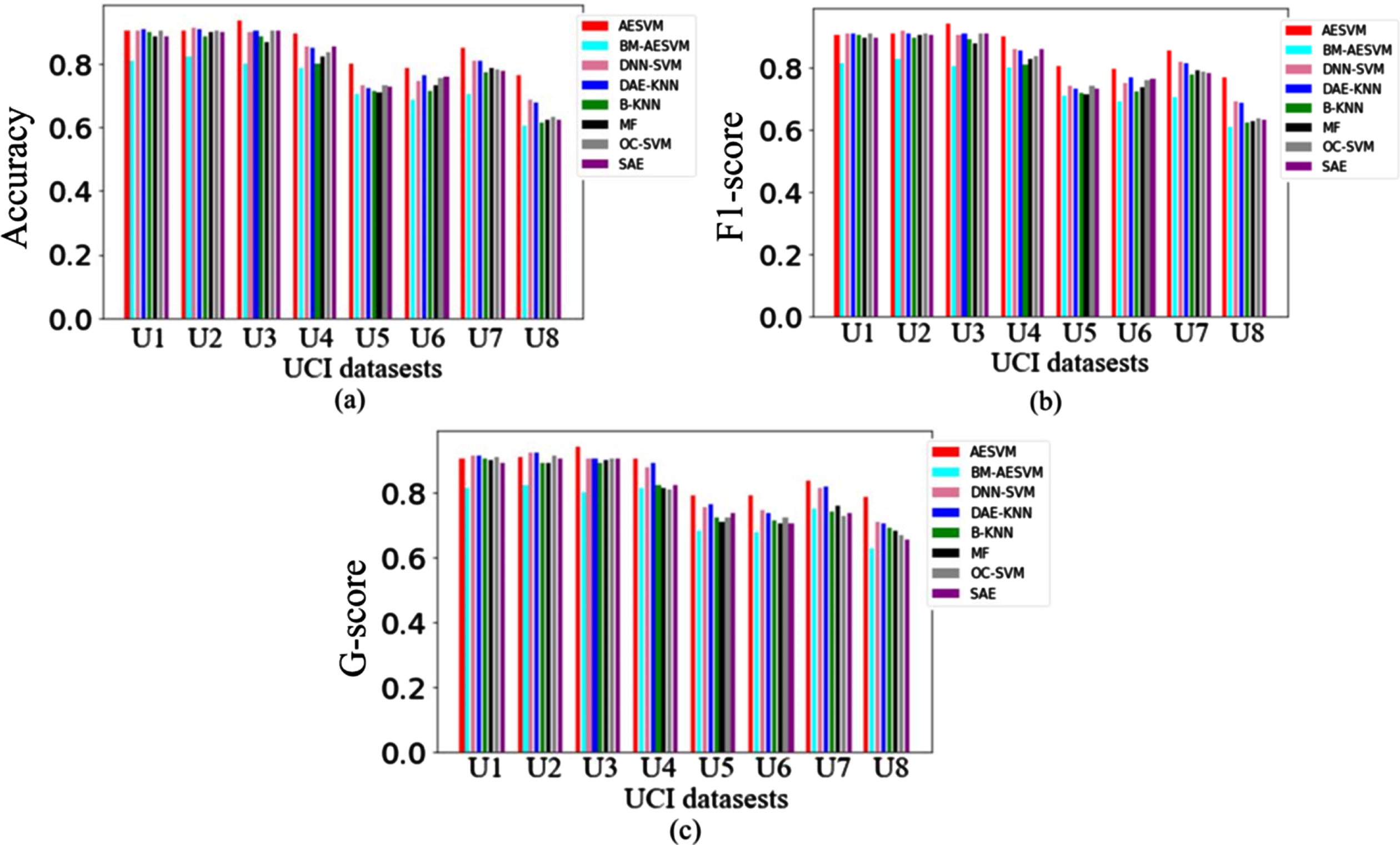
Detected results on the eight UCI datasets. (a), (b) and (c) display the detected results using different assessment metrics.

Results of ablation experiments in Fig. 6 show that the detection ability of AESVM is superior to that of BE-AESVM. Particularly, there are significant differences in detection performance as the dimensions of dataset U1-U8 increases. Unfortunately, on dataset U8 (dimension = 5408), BE-AESVM obtains poor detection performance. This implies that even the hybrid model based on deep network structures is vulnerable to negative effects of high dimensions. By contrary, AESVM suffers less such negative impact because of implementing the dot product operation. Together, these confirm that the proposed dot product operation is beneficial for the model to resist the curse of dimensionality to a certain extent.

Fig. 6

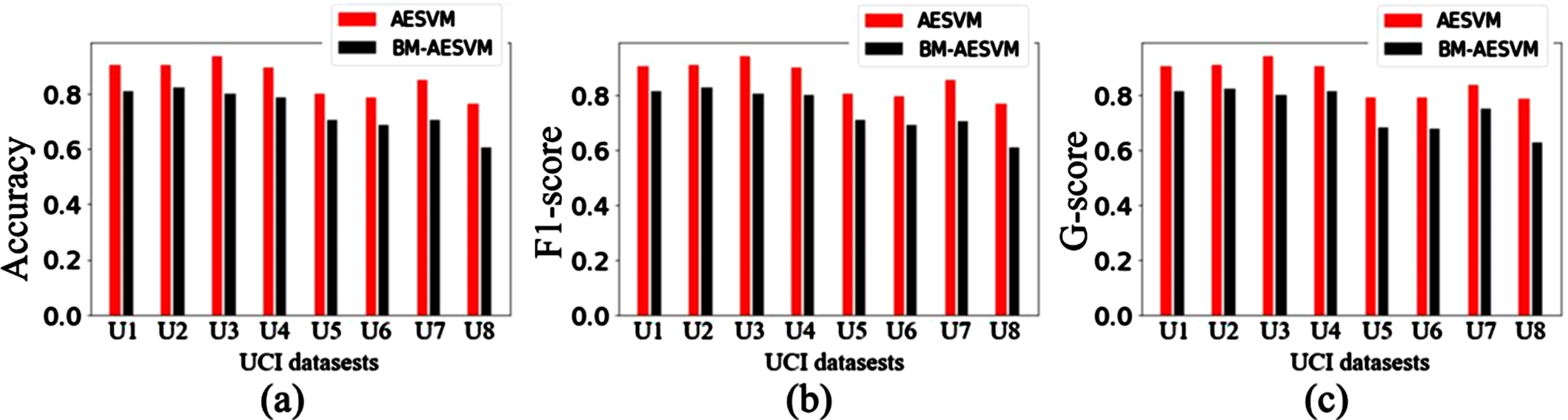
Results of ablation experiments.

4.3 Analysis of affected indicators

Figure 7 unveils that the eight models (AESVM, the benchmark model BE-ASESVM and the six competitive models) begin to drop in detection performance as noise ratio increases or when data dimensionality increases. Nevertheless, AESVM is still better than BE-ASESVM and the six competitors in detection performance. Because our AESVM utilized the Chebyshev theorem to estimate the number of anomalies, which alleviates noise interference to a certain extent. Compared Fig. 7(a) with Fig. 7(b), it can be seen that the noise has more negative effects on the eight methods than data dimensionality does. Hence, suppressing noise interference is more effective than overcoming the curse of dimensionality in improving detection accuracy.

Fig. 7

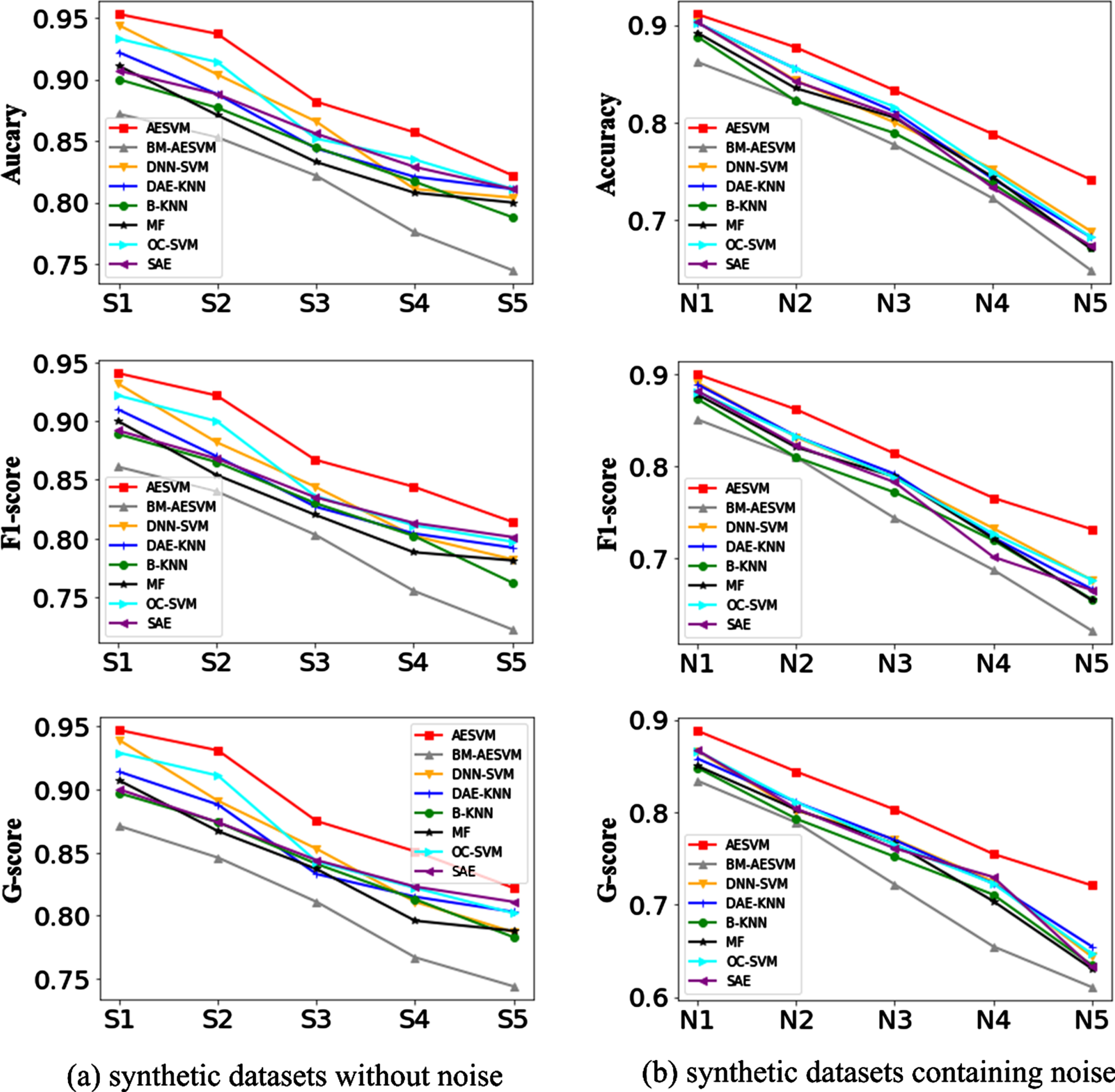
Comparison of negative indicators.

4.4 Discussions

Advantages . Compared with the competitors, the proposed AESVM show more advantages aiming at anomaly detection upon a high-dimensional space. This is because the low-dimensional features extracted by the autoencoder provide favorable space environments for the SVM. In the extracted low-dimensional features, the kernel in Eq. (5) achieves the separation anomaly features from normal features, and Chebyshev’s theorem controls the proportion of anomalies. More importantly, the dot product operation in Eq. (2) can strengthen the learning of AESVM to class labels.

Limitations. AESVM also has shortcoming, for instance, the quality of the extracted features has important effects on the learning ability. Additionally, for most detection methods, the lack of real-world datasets is another major indicator of affecting the accuracy of anomaly detection, so that those detection methods may difficultly reflect the performance of anomalous detection in actual applications.

Insights. Currently, for anomaly detection methods, e.g., Distance measurement-based methods KNN [18, 19], such methods can work in low-dimensional representation spaces well, unfortunately, the detection ability is limited because they are difficult to measure the distance between data in a high-dimensional space. While for deep hybrid -based methods, e.g., DNN-SVM [41], and DAE-KNN [42], deep networks can aid in extracting features. Due to combine with those linear or nonlinear modes, hybrid methods have better scalable, which provide important efforts aiming at building robust anomaly detectors upon complex high-dimensional spaces. Once the combined methods rely on data distribution or easily fall into over-fitting, the capabilities of hybrid methods suffer negative effects. For example, DBN-Random Forest [58] falls into over-fitting since Random Forest easily suffers the risk of over-fitting

5 Conclusion

This paper proposed a hybrid method of combining the autoencoder with the SVM aiming at anomaly detection upon a high-dimensional space. The key thought is that using the autoencoder extracts the features from high-dimensional data, then the SVM achieves the separation of abnormal features and normal features. To increasing the mined precision of abnormal features, Chebyshev’s theorem is used to estimate the upper of the number of abnormal features. Meanwhile, the dot product operation is proposed to strengthen the learning of the model to class labels. Experiment results show that our method gain that the detected accuracy is 0.766, when the data dimensionality is 5408. Numeral results indicate that our method defeats competitors in detected performance for the considered cases. The findings indicate that the reinforcement learning of class labels improve the ability of detectors to detect anomalies. In terms of noise resistance and overcoming the curse of dimensionality, the former can carry out more efforts than the latter. In future work, we will explore anomaly detection under noise interference. Noise can mask anomalies so that anomalies encounter much trap during mining process.

Data availability

Data will be made available on request. The data is cited at http://archive.ics.uci.edu/ml/datasets.php?format=&task=&att=&area=&numAtt=&numIns=&type=mvar&sort=nameUp&view=table

Ethical approval

This manuscript does not contain any studies with human participants or animals performed by any of the authors.

Competing interests

The authors declare no conflict of interest.

Contributions

Zhuo Jiang proposed the methodology and wrote the manuscript. Xiao Huang implemented the source code. Zhuo Jiang, Rongbin Wang designed the experiment.

Footnotes

Appendix

References

Venkataramanan

, Peng

K.C.

, Singh

R.V.

and Mahalanobis

, Attention guided anomaly localization in images[C], In Proc Eur Conf Comput Vis, 2020, pp. 485–503.

Park

, Noh

and Ham

, Learning memory-guided normality for anomaly detection[C], In Proc IEEE Conf Comput Vis Pattern Recognit, 2020, pp. 14360–14369.

Pan

, Chen

, He

, Meng

and Fan

, TCDesc: Learning topology consistent descriptors for image matching, IEEE Trans Circuits Syst Video Technol 32(5) (2022), 2845–2855.

Pan

, Bai

, He

and Zhang

, AAGCN: Adjacency-aware graph convolutional network for person re-identification, Knowl. Based Syst., to be published, 236(25), 1–5.

, Li

, Du

and Tao

, Low-rank and sparse decomposition with mixture of gaussian for hyperspectral anomaly detection, IEEE Trans. Cybern 51(9) (2021), 4363–4372.

Zhang

J.P.

, et al., Viral pneumonia screening on chest X-ray images using confidence-aware anomaly detection, 2020, arXiv:2003.12338.

Chao Huang , Zehua Yang , Jie Wen , Yong Xu , Qiuping Jiang , Jian Yang and Yaowei Wang , Self-Supervision-Augmented Deep Autoencoder for Unsupervised Visual Anomaly Detection, IEEE Transactions on Cybernetics 52(12) (2022), 13834–13847.

Kui Yu and Huanhuan Chen , Markov Boundary-Based Outlier Mining [J], IEEE Transactions on Neural Networks and Learning Systems 30 (2019), 1259–1264.

Vishnu Menon and Sheetal Kalyani , Structured and Unstructured Outlier Identification for Robust PCA: A Fast Parameter Free Algorithm [J], IEEE Transactions on Signal Processing 67 (2019), 2439–2452.

10.

Feng

, Evolutionary multitasking via explicit autoencoding, IEEE Trans Cybern 49(9) (2019), 3457–3470.

11.

Zhang

, Yao

, Chen

, et al., Making sense of spatio-temporal preserving representations for EEG-based human intention recognition, IEEE Trans Cybern 20(7) (2020), 3033–3044.

12.

Sarah Erfanin

, Sutharshan Rajasegarar , Shanika Karunasekera , et al., High-dimensional and large-scale anomaly detection using a linear one-class SVM with deep learning, Pattern Recognition 58 (2016), 121–134.

13.

Khalid Elbaz , Wafaa Mohamed Shaban , Annan Zhou , et al., Real time image-based air quality forecasts using a 3D-CNN approach with an attention mechanism, Chemosphere 333 (2023), 138867.

14.

Khalid Elbaz , Ibrahim Hoteit , Wafaa Mohamed Shaban , et al., Spatiotemporal air quality forecasting and health risk assessment over smart city of NEOM, Chemosphere 313 (2023), 137636.

15.

Khalid Elbaz , Tao Yan , Annan Zhou , et al., Deep learning analysis for energy consumption of shield tunneling machine drive system, Tunnelling and Underground Space Technology, 123 (2022), 104405.

16.

Khalid Elbaz , Shuilong Shen , Annan Zhou , et al., Prediction of Disc Cutter Life During Shield Tunneling with AI via the Incorporation of a Genetic Algorithm into a GMDH-Type Neural Network, Engineering 7(2) (2021), 238–251.

17.

Lin Feng , Huibing Wang , Bo Jin , Haohao Li , Mingliang Xue and Le Wang , Learning a Distance Metric by Balancing KL-Divergence for Imbalanced Datasets, IEEE transaction on Systems, Man, and Cybernetics: Systems 49(12) (2019), 2384–2395.

18.

Shan Zhong , Zongming Bao , Shengrong Gong and Kaijian Xia , Person Reidentification Based on Pose-Invariant Feature and B-KNN Reranking, IEEE Transactions on Computational Social Systems 8(5) (2021), 1272–1281.

19.

Hongchun Qu , Lin Li , Zhaoni Li and Jian Zheng , Supervised discriminant Isomap with maximum margin graph regularization for dimensionality reduction, Expert Systems With Applications 180(2021), 1–17.

20.

Guansong Pang , Longbing Cao , Ling Chen , et al., Learning Representations of Ultrahigh-dimensional Data for Random Distance-based Outlier Detection [C], In KDD, pp. 2041–2050, 2018.

21.

Hu Wang , Guansong Pang , Chunhua Shen , et al., Unsupervised Representation Learning by Predicting Random Distances [C], In Twenty-Ninth International Joint Conference on Artificial Intelligence Main track, pp. 2950–2956, 2020.

22.

Vit Skvára , Tomás Pevny and Václav Smidl , Are generative deep models for novelty detection truly better, ArXiv arXiv:1807.05027, pp. 1–20, 2018.

23.

Jian Zheng , Hongchun Qu , Zhaoni Li , Lin Li and Xiaoming Tang , A deep hypersphere approach to high-dimensional anomaly detection, Applied Soft Computing 125 (2022), 1–17.

24.

Mao

, Wang

and Jin

, Feature grouping-based outlier detection upon streaming trajectories, IEEE Transactions on Knowledge and Data Engineering 29 (2017), 2696–2709.

25.

Jae Beom Ahn , Jin Han Lee , Hong Je Ryoo , Yong Ju Kim , Ki Duk Lee and Jin Lee , PCA-Based Arc Detection Algorithm for DC Series Arc Detection in PV System [C], 2021 24th International Conference on Electrical Machines and Systems (ICEMS), pp. 1–8, 2021.

26.

Zhiming Xia , Yang Chen and Chen Xu , Multiview PCA: A Methodology of Feature Extraction and Dimension Reduction for High-Order Data, IEEE Transactions on Cybernetics 52(10) (2021), 11068–11080.

27.

, Zhang

and Kan

M.Y.

, Fast matrix factorization for online recommendation with implicit feedback [C], In: ACM SIGIR Special Interest Group on Information Retrival, pp. 549–558, 2016.

28.

Yueyang Wang and Bahram Shafai , Nonnegative Matrix Factorization Approach for Image Reconstruction [C], 2021 International Conference on Computational Science and Computational Intelligence (CSCI), pp. 1–8, 2021.

29.

Juncheng Hu , Yongheng Xing , Mo Han , Feng Wang , Kuo Zhao and Xilong Che , Nonnegative matrix tri-factorization based clustering in a heterogeneous information network with star network schema, Tsinghua Science and Technology 27(2) (2022), 386–395.

30.

Jian Zheng , Hongchun Qu , Zhaoni Li , Lin Li and Xiaoming Tao , An irrelevant attributes resistant approach to anomaly detection in high-dimensional space using a deep hyper sphere structure, Applied Soft Computing 116 (2022), 1–20.

31.

Stanley Fong and Sriram Narasimhan , An Unsupervised Bayesian OC-SVM Approach for Early Degradation Detection, Thresholding, and Fault Prediction in Machinery Monitoring, IEEE Transactions on Instrumentation and Measurement 71 (2022), 1–7.

32.

Lu Zhang , Reginald Cushing , Cees de Laat and Paola Grosso , A real-time intrusion detection system based on OC-SVM for containerized applications[C], 2021 IEEE 24th International Conference on Computational Science and Engineering (CSE), pp. 1–10, 2021.

33.

Rabhi Ilham , Roussy Agnès and Pasqualini François , Optimization of OC-SVM engine used for out-of-control detection in semiconductor industry[C], 2022 33rd Annual SEMI Advanced Semiconductor Manufacturing Conference (ASMC), pp. 1–8, 2022.

34.

Feng

, Evolutionary multitasking via explicit autoencoding, IEEE Trans Cybern 49(9) (2019), 3457–3470.

35.

Zhang

, Yao

and Chenl

, Making sense of spatio-temporal preserving representations for EEG-based human intention recognition, IEEE Trans Cybern 20(7) (2020), 3033–3044.

36.

Lukas Ruff , Nico Görnitz and Lucas Deecke , Deep one-class classification[C], In International Conference on Machine Learning, pp. 4390–4399, 2018.

37.

Peng Peng , Wenjia Zhang , Yi Zhang , Hongwei Wang and Heming Zhang , Imbalanced Fault Diagnosis Based on Particle Swarm Optimization and Sparse Auto-Encoder[C], 2021 IEEE 24th International Conference on Computer Supported Cooperative Work in Design, pp. 1–6, 2021.

38.

Yang Liu , Jing Liu , Jieyu Lin , Mengyang Zhao and Liang Song , Appearance-Motion United Auto-Encoder Framework for Video Anomaly Detection, IEEE Transactions on Circuits and Systems II: Express Briefs 69(5) (2022), 2498–2502.

39.

Peng Gao , Gu Feng and Fei Liang , Anomaly Detection in Dynamic Graph based on Deep Graph Auto-encoder[C], 2022 International Conference on Machine Learning and Intelligent Systems Engineering (MLISE), pp. 1–6, 2022.

40.

Xinwei Jiang , Junbin Gao and Xia Hong , Gaussian processes autoencoder for dimensionality reduction[C], In PAKDD, pp. 62–73, 2014.

41.

Jun Inoue , Yoriyuki Yamagata and Yuqi Chen , Anomaly detection for a water treatment system using unsupervised machine learning[C], In Data Mining Workshops 2017 IEEE International Conference on, pp. 1058–1065, 2017.

42.

Hongchao Song , Zhuqing Jiang and Aidong Men , A hybrid semi-supervised anomaly detection model for high-dimensional data, Computational Intelligence and Neuroscience, pp. 1–9, 2017.

43.

Sangwook Kim , Yonghwa Choi and Minho Lee , Deep Learning with Support Vector Data Description, Neurocomputing 165 (2015), 111–117.

44.

Jun Inoue , Yoriyuki Yamagata and Yuqi Chen , Anomaly detection for a water treatment system using unsupervised machine learning[C], In Data MiningWorkshops 2017 IEEE International Conference on, pp. 1058–1065, 2017.

45.

Shenglong Zhou , Sparse SVM for Sufficient Data Reduction, IEEE Transactions on Pattern Analysis and Machine Intelligence 44(9) (2022), 5560–5571.

46.

Mengyu Yang , Shigang Cui , Yongli Zhang , Jingyu Zhang and Xinqi Li , Data and Image Classification of Haematococcus pluvialis Based on SVM Algorithm[C], 2021 China Automation Congress (CAC), pp. 1–10, 2021.

47.

Bengio

and LeCun

, Scaling learning algorithms towards AI[C], In: L. Bottou, (Eds.), Large Scale Kernel Machines, pp. 1–41, 2007.

48.

Raghavendra Chalapathy and Sanjay Chawla , Deep Learning for Anomaly Detection: A Survey[J], arXiv:1901.03407v2, 2019, 1–50.

49.

Guansong Pang , Chunhua Shen , Longbing Cao , et al., Deep Learning for Anomaly Detection: A Review[J], arXiv:2007.02500v3, 2020, 1–36.

50.

Degang Chen , Hengyou Wang and Eric Tsang

C.C.

, Generalized Mercer Theorem and its application to feature space related to indefinite kernels[C],2008 International Conference on Machine Learning and Cybernetics, 2008:1–1.

51.

Sadeep Jayasumana , Richard Hartley , Mathieu Salzmann , et al., Optimizing Over Radial Kernels on Compact Manifolds[C], Proceedings of the IEEE Conference on Computer Vision and Pattern Recognition, pp. 3802–3809, 2014.

52.

Brett Amidan

, Thomas Ferryman

and Cooley

, Data Outlier Detection using the Chebyshev Theorem[C], IEEE Aerospace Conference 2005, 2005:1–6.

53.

Xinjun Peng and Dong Xu , A twin-hypersphere support vector machine classifier and the fast learning algorithm[J], Information Science 221 (2013), 12–27.

54.

Snoek , Jasper , Swersky , et al., Ryan. Input warping for bayesian optimization of non-stationary functions[C], In International Conference on Machine Learning, 2014:1674–1682.

55.

Jayasumana

, Hartley

, Salzmann

, et al., Kernel Methods on the Riemannian Manifold of Symmetric Positive Definite Matrices[C], In CVPR, 2013:1–1.

56.

Campos

G.O.

, Zimek

, Sander

, et al., On the evaluation of unsupervised outlier detection: measures, datasets, and an empirical study[J], Data Mining & Knowledge Discovery 30 (2016), 891–927.

57.

Johansson

and Lofstrom

, Producing implicit diversity in ANN ensembles[C], In Neural Networks (IJCNN), 2012 International Joint Conference on, 2012:1–8.

58.

Tin Kam Ho , Random decision forests[C], Document Analysis and Recognition, Proceedings of the Third International Conference on 1 (1995), 278–282.