Research on flame detection method based on improved SSD algorithm

Abstract

A flame detection algorithm based on the improved SSD (Single Shot Multibox Detector) is proposed in response to the issues with the limited detection distance, delayed reaction, and high false alarm rate of previous flame detection systems. First, the ResNet-50-SPD model was added to the original backbone network to improve the detection of low resolution and tiny objects. After that, incorporate feature fusion between layers to improve the bond between contexts. Before the feature entered the prediction, the impact of channel number reduction was eliminated using the adaptive module AAM. According to experimental findings, the modified SSD algorithm’s mAP value on on the random division dataset and K-fold verification dataset reaches 87.89% and 89.63%, respectively, which is 3.97% and 5.17% higher than the original SSD, while the FPS remains at 64.9 f/s. It is helpful to improve the time of the fire alarm, find the ignition point in time, and better meet the actual engineering needs of fire monitoring.

Keywords

Flame detection SSD ResNet-50-SPD feature fusion AAM

1 Introduction

Fire is a highly frequent and readily sparked environmental catastrophe that frequently poses a serious threat to public safety and the security of private property in various industrial operations. Building a more precise and efficient way to recognize flames is of utmost importance for the avoidance of fire accidents since fire mishaps are distinguished by their suddenness and wide range of hazards. Traditional fire detection primarily uses sensors for flame detection. Flame prediction is carried out by sensing temperature and smoke, which can summarize the information in the space, and then further assess the situation of the fire and respond. Unfortunately, when the environment is complicated and far from the fire, it is challenging to use the sensor properly.

In recent years, computer technology has grown significantly. AlexNet, a deep learning neural network, debuted in 2012 and immediately garnered popularity [1]. The convolution neural network is being utilized in image processing more and more frequently as a result of researchers’ increased focus on deep learning. The deep learning-based target detection system has a high detection accuracy and speed and can learn the target features independently. The way rectangular boxes are created during detection can be used to categorize these algorithms into one-stage and two-stage processes. The YOLO (You Only Look Once) [2] series and the SSD (Single Shot Multibox Detector) [3] algorithm are typical one-stage algorithms, while the R-CNN (Region-Based Convolutional Neural Network) [4], Fast R-CNN (Fast Region-Based Convolutional Neural Network) [5], Faster R-CNN (Faster Region-Based Convolutional Neural Network) [6] are representative algorithms of the two-stage algorithms.

The idea of applying deep learning to the task of flame detection is a critical research direction. Convolution neural networks (CNN) are used by Frizzi et al. [7, 8]. Automatic extraction of flame features for the purpose of detecting flame targets, although the features extracted and the detection outcomes are not optimal. Long Short-Term Memory (LSTM) [9] network was utilized by Kim et al. [10] to classify after detecting suspicious flame areas using the spatial properties of Faster R-CNN, which boosted detection accuracy but added computation and slowed down detection. By examining the number of fire modules and their placements in the model, Fang et al. [11] created a little detection network based on Tinier-YOLO to discover flames, but the detection platform is complex and expensive. Li et al. [12] designed a fused MobileNetV3 network with a frame-free structure. After lightweight, the model detection speed is significantly improved, but the detection accuracy is decreased. Sun et al. suggested an enhanced YOLOv4 flame detection algorithm that utilizes CSPDarkNet53 (Cross Stage Partial Networks53) as the backbone network and improves the feature extraction network through the use of SPP (Spatial Pyramid Pooling) and PANET (Path Aggregation Network) structures [13–16]. Despite a substantial increase in detection accuracy, real-time requirements are still not satisfied. Jeon et al. [17] achieved a 97.9% F1 score by detecting fire using a CNN based on a multi-scale prediction framework. This work demonstrates that multi-scale prediction can effectively assist in the robustness and universality of fire detection. Wu et al. [18] proposed a video fire detection method based on improved YOLOv5. This method introduces a cavity convolution module in YOLOv5’s SPP module to improve the ability of feature extraction and small-scale object detection, in order to accurately detect small-scale flames in the early stages of a fire. Qin et al. [19] proposed a fire detection method that combines classification models and object detection models. The method uses deep separable convolution to classify fire images, and then uses the YOLOv3 model’s object regression function to determine the fire location of the image. Xu et al. [20] proposed an ensemble learning method to detect forest flames, and used the ensemble model to comprehensively score to identify flames, which reduced the false alarm rate to a certain extent, but the network structure was very complex, resulting in detection speed slower. Majid et al. [21] proposed a user-defined framework using Transfer learning, which uses the most advanced cellular neural network trained on the real-world fire outbreak image to detect fires, and also uses gradient CAM method to visualize and locate fires in the image. And an attention mechanism is used, which greatly helps the network achieve better performance.

Real-time is necessary for the real-time detection of flame images, and it is challenging to extract the characteristics of complicated flame features. This paper enhances the SSD algorithm to enhance flame detection speed and precision. Resnet-50-SPD, which is based on the original SSD algorithm, replaces VGG-16 as the SSD algorithm’s new backbone network and includes feature fusion between layers [22, 23]. The feature extraction layer is then supplemented with AAM (Attention Adaptation Module) [24] following fusing.

2 SSD target detection algorithm

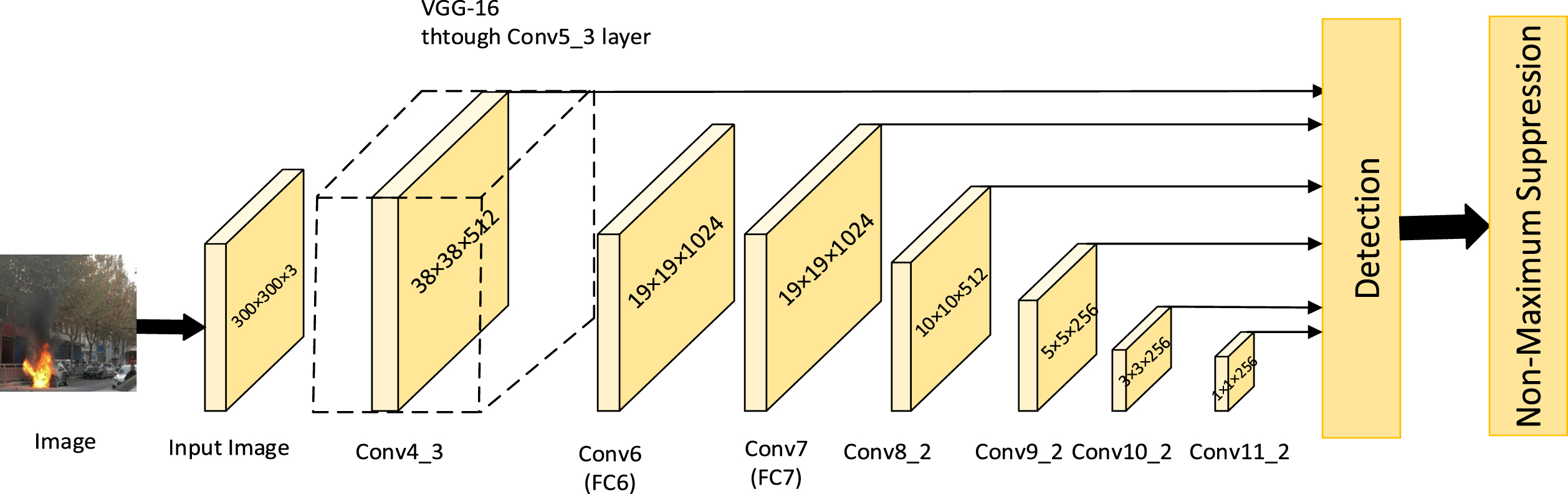
The SSD algorithm’s primary function is to oversample image locations, which is similar to the Faster R-CNN idea of a candidate box. The object bounding box is predicted by a priori box with varying scales and aspect ratios during sampling. Next, CNN extracts the features, which are then immediately classified and regressed. The SSD network employs six feature maps for the recognition and convolutional resizing of images. For target identification, it makes use of pyramid-structured feature layer groups. Large targets are predicted using high-level feature maps from deep SSD networks, whereas tiny targets are predicted using low-level feature maps from bottom networks. The first five levels of the VGG-16 network remain the SSD network’s foundation. The middle two full connection layers, Fc6 and Fc7, are replaced by two convolution layers to acquire the feature information for the complete picture because the entire connection layer interferes with the location information extraction of the model’s features. To acquire characteristic information at various scales, the back of the device has four convolution layers attached. The convolution kernel with a width of 1 × 1 is used for down sampling, and the convolution kernel with a width of 3 × 3 is used for feature information extraction for each set of convolution layers.

Fig. 1

Original SSD network model.

After the input image passes through the backbone network and feature extraction network, select Conv4_3, Conv7, Conv8_2, Conv9_2, Conv10_2, and Conv11_2 to enter the prediction layer. The number of anchor frames in the prediction layer is 4, 6, 6, 6, 4, and 4. The prior frame on each feature point passes through a convolution layer with a convolution kernel size of 3 × 3. After calculation, the anchor frame’s offset and category confidence are found. Adjust the prior box according to the size of the offset to get the prediction box, and filter out the prediction box that is most likely to contain the target according to the threshold. Finally, the position and specific category of the target in the image are obtained through non-maximum suppression (NMS) [25]. The network structure is shown in Fig. 1. The SSD algorithm recognizes things of various sizes using features at multiple scales. The algorithm adopts anchor box processing, and all the center points on the feature layer generate a succession of default boxes with multiple sizes. The size of the default box for each feature layer can be expressed as Equation (1), where K ∈ [1, m]. $S_{K} = S_{min} + \frac{S_{max} - S_{min}}{m - 1} (K - 1)$ (1)

Where S_min = 0.2 is the size of the shallow default box, S_max = 0.9 is the size of the deep default box, and m is the number of layers of the feature extraction layer. In the SSD algorithm, m = 6. Use different aspect ratios value to get different default boxes, where the aspect ratio includes a_γ ∈ {1 : 1, 1 : 2, 2 : 1, 1 : 3, 3 : 1}.

As far as the position of the target is concerned, it is necessary to introduce an intersection in the union, namely Intersection over Union (IoU) [26]. Determine whether the recognition result is normal or negative and whether the recognition is correct. It is usually used in the evaluation of current target detection algorithms. The higher the value IoU, the better the detection effect of the algorithm. The formula is as follows: $IoU = \frac{G_{t} \cap D_{r}}{G_{t} \cup D_{r}}$ (2)

G_t is the area of the real frame, and D_r is the area of the predicted frame. G_t ∩ D_r is the intersection of G_t and D_r, and G_t ∪ D_r is the union of G_t and D_r. The range of IoU is 0 to 1. In this article, IoU is set to 0.5. Once the detection position and label position are reached, the target position will be determined accordingly.

Equation (3) is the loss function of network training consists of two parts, namely, the category loss function and the position loss function corresponding to the target. $L (x, c, l, g) = \frac{1}{N} (L_{conf} (x, c) + α L_{loc} (x, l, g))$ (3)

Where N is the number of positive samples in the default box. If N = 0, set the loss to 0, x is the category matching result of the detection frame; l is the position information of the detection frame; c represents the confidence of category detection; g is the true information of the detection frame; α is its weight coefficient, which is used to adjust the proportion of category loss and location loss. The default is α = 1. $L_{conf} (x, c) = - \sum_{i \in Pos}^{N} x_{ij}^{p} log ({\hat{c}}_{j}^{p}) - \sum_{i \in Neg} log ({\hat{c}}_{i}^{o})$ (4) ${\hat{c}}_{i}^{p} = \frac{exp (c_{i}^{p})}{\sum_{p} exp (c_{i}^{p})}$ (5)

In Equations (4) and (5), L_conf represents the category loss function of the target. Where i refers to search box information, j refers to real box information, p refers to category information, and p = 0 refers to the background. $X_{ij}^{p}$ represents the information that the jth real frame is matched by the ith detection frame on the category p, $C_{i}^{p}$ predicts the probability of category p corresponding to the ith search box. i ∈ Pos is the loss of positive sample and i ∈ Neg is the loss calculation of the category is the loss value under the background. $L_{loc} (x, l, g) = \sum_{i \in Pos}^{N} \sum_{m \in (cx, cy, w, h)} x_{ij}^{k} smoot h_{L 1} (l_{i}^{m} - {\hat{g}}_{j}^{m})$ (6) $smoot h_{L 1} (x) = {\begin{matrix} 0.5 x^{2} & if | x | < 1 \\ | x | - 0.5 & otherwise \end{matrix}$ (7)

In Equations (6) and (7), L_loc is the position loss function of the target, and is the smooth_L1 loss between the parameters of the actual box (g) and the prediction box (l). The use of smooth_L1 loss is to prevent gradient explosion in the early stage of training and quantify the error in the position between the prior frame and the real frame.

3 Improved SSD network model

The VGG-16 network serves as the detection model’s structural foundation in the initial SSD model. VGG-16 comprises a series of convolution layers, pooling layers, and complete connection layers. The most crucial aspect of VGG-16 is its extremely straightforward construction. When building a network, it can be achieved only by overlaying multiple convolution layers and pooling layers. Its drawbacks include the shallow number of layers in the VGG-16, the oversimplified network structure, the reliance on a small number of convolution layers for feature extraction, and the performance issues. Additionally, the network model contains a lot of redundant calculations, especially when detecting small targets. Based on the SSD framework, ResNet-50-SPD is used as the backbone network of the algorithm, and feature fusion is added between layers. After fusion, AAM module is added to the feature extraction layer.

Each step convolution layer and each pooling layer are replaced by a new CNN block in the ResNet-50-SPD network by SPD-Conv. A series of feature layers at the back can also hold more semantic information to enhance the detection effect of small targets. Feature fusion can combine low-level features into high-level features. The AAM adaptive module then processes the generated prediction feature layer, which can decrease the loss of context information in the high-level feature map brought on by the reduction of feature channels. Finally, NMS is used to determine the location and precise category of the target in the image. The improved SSD model structure is shown in Fig. 2 below.

Fig. 2

Improved SSD network model.

3.1 Resnet-50-SPD network structure

ResNet network was proposed by He and others in 2016 [27]. Precision degradation when the network structure adds more layers is addressed by ResNet networks built on residual thought. The majority of the images studied have high resolution and moderate object sizes, so there is a large amount of redundant pixel information, which can be easily skipped across convolution and pooling operations and can still learn features well. As a result, the negative effects of residual structure and pooled layer used in the shallow layer of CNN structure are typically not shown. However, when the image is blurred, or the object is small, the over-assumption of redundant information is no longer tenable, resulting in the loss of small information and reduced learning efficiency. To this end, SPD-Conv is added to the ResNet network to build a new CNN block to replace each cross-convolution layer and each pooling layer (so as to eliminate them completely). SPD-Conv down-samples the feature map without losing learnable information and no longer uses cross-domain convolution and pooling operations. For low-resolution images and small objects, the performance is significantly improved when the detection is difficult.

In this paper, ResNet-50-SPD is selected as the backbone network of SSD algorithm, and ResNet-50 is selected and modified to make the network performance better. The first change is to select only Conv1 to Conv4_x layer structures as backbones to improve the low-level feature extraction ability. Removing Conv5_x and the layer structure behind it can solve the problem that the full-connected layer will limit the size of the input image and reduce the calculation amount. The second change is to use SPD-Conv to replace the pooling layer and shortcut branch in ResNet-50. The SPD layer down-sampling the characteristic graph X can preserve all information in the channel and prevent information loss. The third change is to change the convolution step in Conv4_x to 1, so as not to reduce the size of the feature map by half after passing Conv4, and keep the output size at 1, to obtain more feature information. The structure diagram show in Table 1.

Table 1
ResNet50-SPD architecture

Layer name ResNet-50-SPD

Spd1 SPD-Conv

Conv1 3 × 3, 64

Conv2-x $[\begin{matrix} 1 \times 1, 64 \\ 3 \times 3, 64 \\ 1 \times 1, 256 \end{matrix}] \times 3$

Spd2 SPD-Conv

Conv3-x $[\begin{matrix} 1 \times 1, 128 \\ 3 \times 3, 128 \\ 1 \times 1, 512 \end{matrix}] \times 4$

Spd3 SPD-Conv

Con4-x $[\begin{matrix} 1 \times 1, 256 \\ 3 \times 3, 256 \\ 1 \times 1, 1024 \end{matrix}] \times 6$

Spd4 SPD-Conv

Layer name	ResNet-50-SPD
Spd1	SPD-Conv
Conv1	3 × 3, 64
Conv2-x	$[\begin{matrix} 1 \times 1, 64 \\ 3 \times 3, 64 \\ 1 \times 1, 256 \end{matrix}] \times 3$
Spd2	SPD-Conv
Conv3-x	$[\begin{matrix} 1 \times 1, 128 \\ 3 \times 3, 128 \\ 1 \times 1, 512 \end{matrix}] \times 4$
Spd3	SPD-Conv
Con4-x	$[\begin{matrix} 1 \times 1, 256 \\ 3 \times 3, 256 \\ 1 \times 1, 1024 \end{matrix}] \times 6$
Spd4	SPD-Conv

SPD-Conv consists of space-to-depth (SPD) layer and non-strited revolution (Conv) layer. The SPD layer only down-samples the feature map X, preserving all information in the channel dimension, so it will not lose information. Add a non-step convolution operation after each SPD to reduce the number of channels with learnable parameters in the added convolution layer.

The SPD operation extends the original image conversion technology to the internal and overall downsampling of the feature graph of the convolution neural network. Equation (8) considering any middle feature graph X with size S × S × C₁, a series of sub- feature charts are cut out and calculated from the following formulas: $\begin{matrix} f_{0, 0} = X [0 : S : scale, 0 : S : scale] \\ f_{1, 0} = X [1 : S : scale, 0 : S : scale], . . ., \\ f_{scale - 1, 0} = X [scale - 1 : S : scale, 0 : S : scale]; \\ f_{0, 1} = X [0 : S : scale, 1 : S : scale], f 1, 1, . . ., \\ f_{scale - 1, 1} = X [scale - 1 : S : scale, 1, S, scale]; \\ . . . \\ f_{0, scale - 1} = X [0 : S : scale, scale - 1 : S : scale], \\ f_{1, scale - 1}, . . ., \\ f_{scale - 1, scale - 1} = X [scale - 1 : S : scale, scale - 1 : S : scale] \end{matrix}$ (8)

In general, given any characteristic graph x, the f_x,y subgraph is formed from all entries X (i, y) of i + x and i + y that can be proportionally divisible. Therefore, each subgraph is down sampled by the scale factor X. Figure 3 gives the sampling result when scale = 2 is used and four subgraphs are f_0,0, f_1,0, f_0,1, f_1,1.

Fig. 3

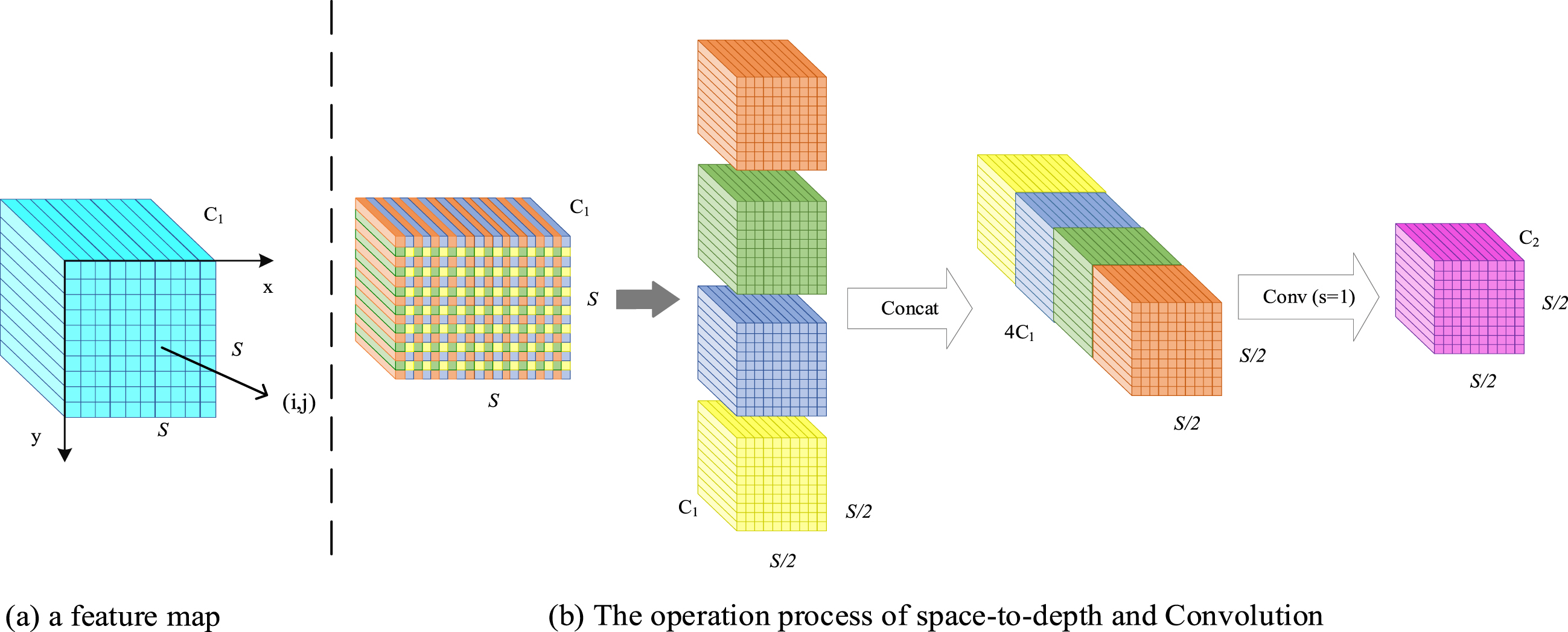
Schematic diagram of SPD-Conv when scale = 2.

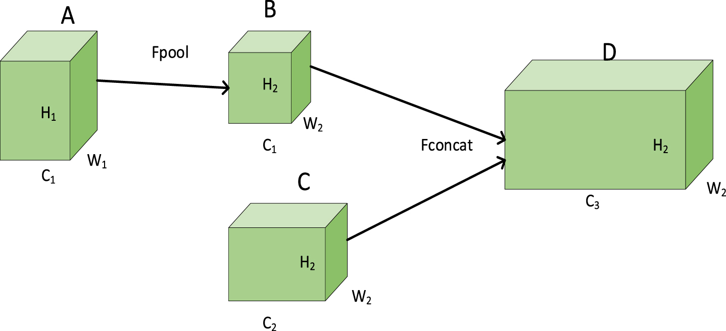
Each of these sub-feature maps has a size of (S/2, S/2, C₁), and then these sub-feature maps are stitched together in the channel dimension using Concat operations to obtain the feature figure X′. This reduces the spatial dimension by a scale factor and increases the channel dimension by a scale factor of 2. In other words, SPD converts the feature X (S, S, C₁) into the intermediate feature $X^{'} (\frac{S}{scale}, \frac{S}{scale}, scal e^{2} C_{1})$ . After the SPD feature transformation layer, a convolution layer with step 1 of C₂ filter is added, of which and $X^{'} (\frac{S}{scale}, \frac{S}{scale}, scal e^{2} C_{1}) \to X′′ (\frac{S}{scale}, \frac{S}{scale}, C_{2})$ are further transformed. The convolution operation with step 1 preserves all discriminant feature information as much as possible.

3.2 Feature fusion

Figure 4 below shows the feature fusion process from Conv4_3 to Fc7. The feature map at Conv4_3 is represented by A ∈ R^{W₁×H₁×C₁}, and the feature map at Fc7 is C ∈ R^{W₂×H₂×C₂} [28]. The pooling formula is shown in Equation (9). A to B are transformed by the pooling operation B ∈ R^{W₂×H₂×C₁}. The pooling operation changes the length and width of the feature map in order to facilitate the Concat operation. $\begin{matrix} B_{C} (x, y) = F_{pool} (A_{C}) \\ = max (A_{C} (i, j) | i = x + l, . . ., x + k; j = y + 1, . . ., y + k \end{matrix}$ (9)

Fig. 4

Fusion process.

Where B_C indicates that the number of channels of the feature map B is C, B_C (x, y) indicates that the feature maps have the same width and height, takes the value confirmed by Equation (10). From this, we can deduce that A_C and A_C (i, j), k × k are the dimensions of the pooling kernel and padding is 0. $x = 0, . . ., \frac{W_{1}}{k} - 1; y = 0, . . ., \frac{H_{1}}{k} - 1$ (10)

Then B and C are transformed into D a tandem operation D ∈ R^{W₂×H₂×C₃}.Concat splicing is a concatenated operation that operates only in the channel dimension, without changing the width and height, to get C₃ = C₁ + C₂. After feature fusion, the features of Fc7, Conv6_2, Conv7_2, Conv8_2, and Conv9_2 are added more at lower levels, which contain more se mantic information, and the addition of low-level features containing small target information is beneficial to the subsequent detection of small targets. In the process of feature fusion, it should be noted that Batch Normalization (BN) operations need to be performed before stitching to generate consistent size sizes for different feature mappings [29]. A relatively large gradient can be obtained using the BN layer to solve the problems that occur when the intermediate layers acquire data during the training process. It is used to prevent gradient disappearance or gradient explosion and to speed up the convergence of the network, which can improve the training speed and, in turn, can substantially improve the detection of flames.

3.3 AAM structure

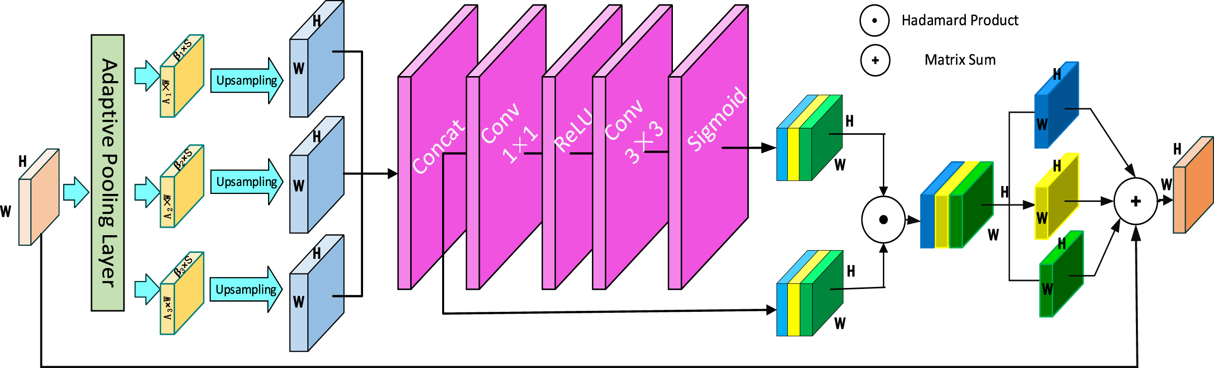
Figure 5 depicts the unique structure of the AAM. First, the input size is H × W for the adaptive attention module. The AAM module’s operation may be broken down into two parts. First, the adaptive pooling layer enables the acquisition of contextual semantic information at various scales. The pooling factor set to [0.1, 0.5], which will make adaptive adjustments based on the target size in the dataset. The adaptive averaging pooling layer adapts the input signal consisting of multiple feature layers to perform adaptive averaging pooling in two dimensions, operating in the height and width dimensions. For any input size, the output size is the height × width. The number of output features equals the number of input feature layers.

Fig. 5

Model structure of AAM.

Second, a spatial weight map generate for each feature map through a spatial attention mechanism. A new feature map containing multi-scale contextual information is generated by fusing contextual features through the weight map. First, 1 × 1 convolution is performed for each contextual feature to obtain the same channel dimension of 256. It is upsampled to a scale S using bilinear interpolation to facilitate the fusion of the three contextual feature channels by the Concat operation. Then the feature maps are sequentially passed through a convolutional layer with a convolutional kernel size of 1 × 1, a ReLU activation function, a convolutional layer of size 3 × 3 and a Sigmoid activation function to generate the corresponding spatial weights for each feature map. After merging channels, the generated weight map and the feature map are subjected to the Hadamard product operation, which is separated and added to the input feature map, combining the contextual features into a new feature map. The resulting feature map will have richer contextual information at multiple scales, which can alleviate the information loss due to the reduced number of channels to a certain extent.

4 Dataset and experimental setup

4.1 Image dataset

So far, there is no more authoritative dataset for the field of flame detection, so in the process of flame image acquisition for this experiment, flame images from different sources are collected in this paper to ensure the diversity and richness of the dataset and to improve the model generalization performance. It contains images intercepted in the public video collection MIVIA [30], flame images collected online using Baidu and Google, and a self-built flame dataset. The flame images in different scenarios are selected, such as car, house, forest, party bonfire, candle, and garbage burning, as shown in Fig. 6. A total of 6,000 flame images were used in the data set. The images were manually labeled using the rectangular box in the LabelImg image labeling method. Every effort was made to mark the edges of the flames within the rectangular box to prevent the problem of being unable to correctly identify the flames during the simulation exercise. The labeling was completed by saving the asked VOC format and stored in txt text.

Fig. 6

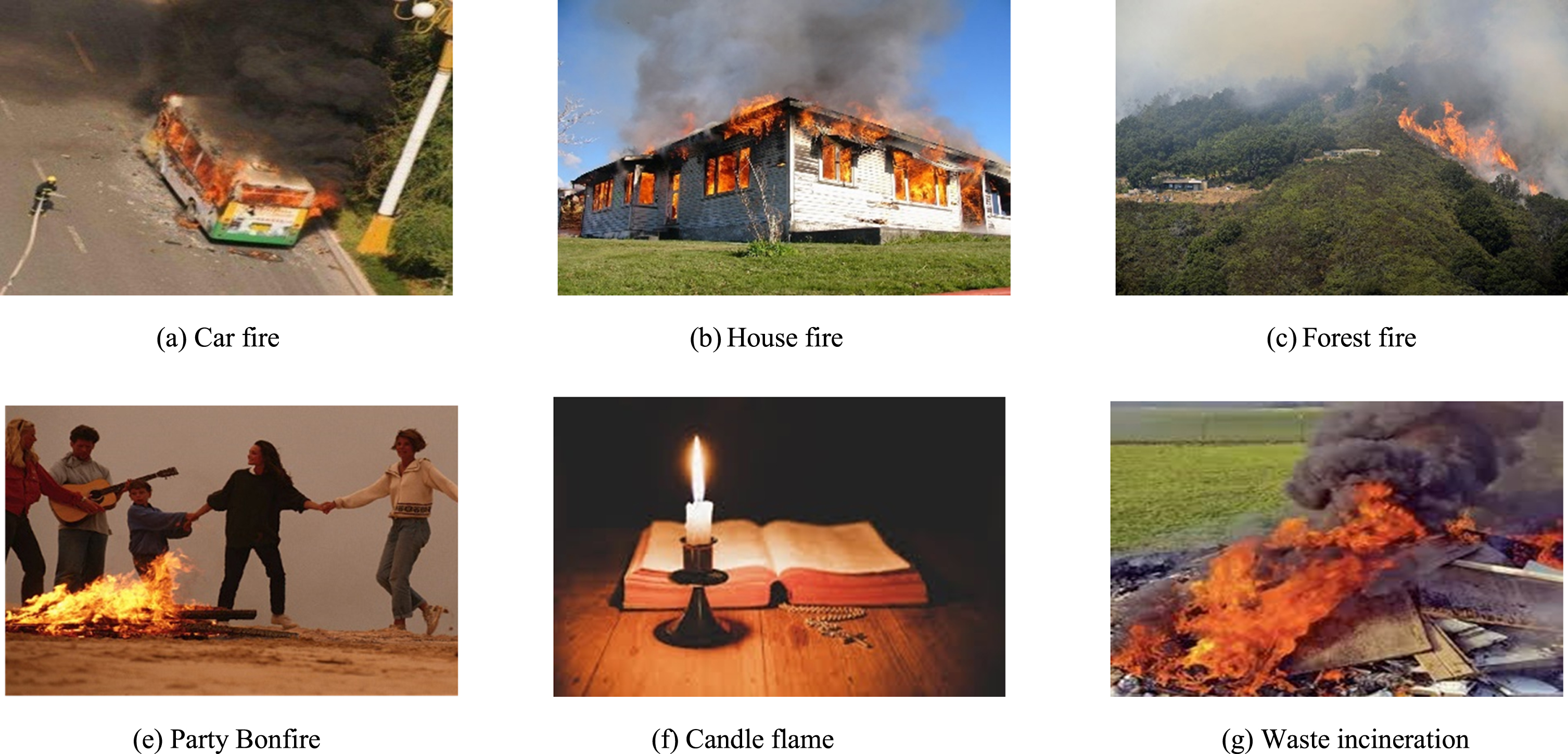
Flame image type in the dataset.

Due to the limited number of images in the homemade fireworks dataset, for the model to better learn the target features and improve the robustness, 90°, 180°, and 270° rotations and horizontal flip operations are made to the images in the training set of the dataset for data enhancement, as shown in Fig. 7. After data augmentation, the dataset was expanded to 24,000 images. The data set is randomly divided into training and test sets in the ratio of 8 : 2, with 19200 images as the training set and another 4800 images as the test set to verify the effectiveness.

Fig. 7

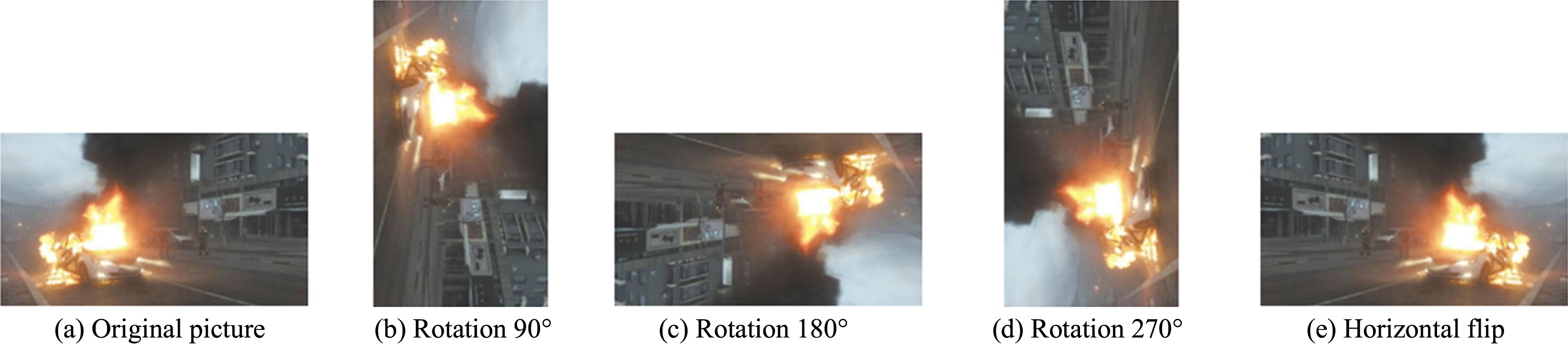
Data Enhancement.

4.2 Hardware environment

The Intel(R) Core(TM) i9-10900 CPU @ 3.70 GHz processor, 128GRAM and Nvidia GeForce RTX 3060 were selected for the experiments. All experiments were performed in pytorch1.9, cuda11.6, python3.7 and win10 environment. The SSD algorithm was the experimental environment was built using the Pytorch environment.

4.3 Training parameters

The SSD algorithm is trained by setting the following parameters, the input image is, the batch_size is set to 16, the learning_rate is set to 0.0005, and a total of 300 iterations are trained.

4.4 Evaluation indicators

Speed is evaluated using frames per second (FPS), and accuracy is evaluated using mean accuracy (mAP). FPS indicates the number of images per second that can be processed by the algorithm, and a higher value of FPS indicates that the algorithm is faster. mAP is the average accuracy for each category, and then the average accuracy is the mean value, as follows Equations (9) and (10). $mAP = \frac{1}{C} \sum_{i = 0}^{C} AP (c)$ (11) $A p = \frac{1}{N} \sum_{r \in {r_{1}, r_{2}, \dots, r_{N}}} p (r)$ (12) where C is the number of types of targets, AP is the average accuracy of targets. N denotes the number of recalls, R = TP/TP + FN denotes the recall rate, and P = TP/TP + FP denotes the maximum accuracy. Definition TP is the number of positive samples detected, FP is the number of detections that are not positive samples as valid targets, and FN is the number of true samples that are not detected.

5 Analysis of results

5.1 Analysis of training results

The total loss change of the model is shown in Fig. 8. With the increase of iteration times, the loss value gradually decreases and tends to be stable, which proves that the recognition accuracy of the model is constantly improving.

Fig. 8

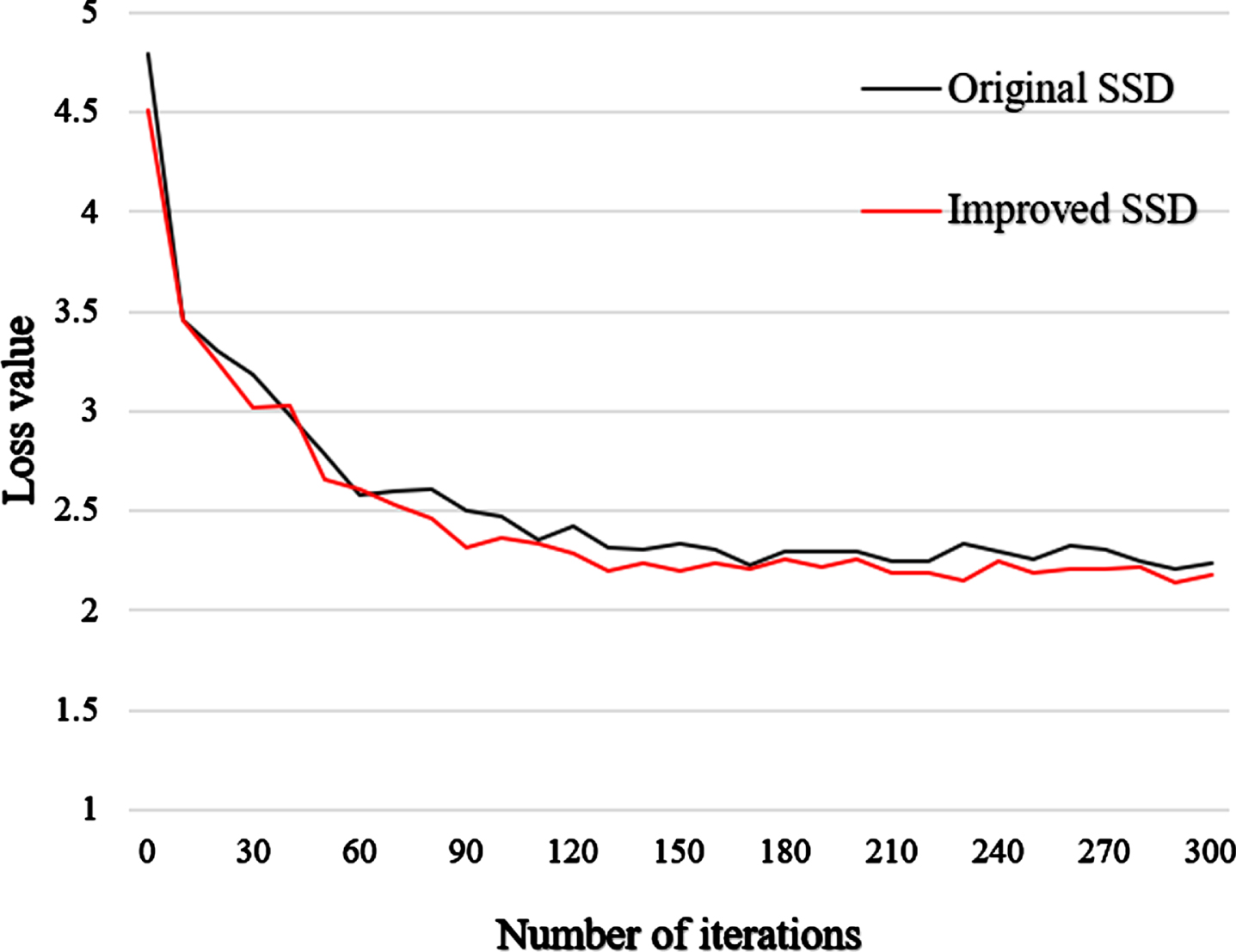
Training loss curve.

5.2 Ablation results and analysis

The focus of this paper is the algorithm that can detect flame identification with high accuracy and real-time, which provides the possibility for practical application. Through the ablation experiment, the effect of different improvement points on the experimental results based on SSD algorithm is verified. The experimental results are shown in Table 2.

Table 2
Results of ablation experiment

Experiment VGG ResNet-50-SPD Feature fusion AAM mAP/% FPS/f/s

1 √ 83.92 65.6

2 √ 84.36 65.1

3 √ √ 85.12 64.6

4 √ √ 86.27 64.1

5 √ √ √ 87.89 62.9

Experiment	VGG	ResNet-50-SPD	Feature fusion	AAM	mAP/%	FPS/f/s
1	√				83.92	65.6
2		√			84.36	65.1
3		√	√		85.12	64.6
4		√		√	86.27	64.1
5		√	√	√	87.89	62.9

Table 2 effectively analyzes all improvement strategies. Experiments 2-5 show that each improvement strategy contributes to the model in varying degrees. Experiment 1 used the original network SSD with VGG as the backbone network for network training, as the control group of experimental data. The mAP is 83.92%, and the FPS is 65.6. In Experiment 2, the original VGG-16 backbone network was replaced by ResNet-50-SPD. Compared with Experiment 1, the mAP value was increased by 0.44%, indicating that the replacement of the backbone network makes the network feature extraction more effective. Experiment 3 added a feature fusion network on the basis of ResNet-50-SPD, achieving a detection accuracy of 85.12%, indicating that the improved feature fusion method made the network training more in-depth. In Experiment 4, an AAM module was added to ResNet-50-SPD, achieving a detection accuracy of 86.27%, indicating that the AAM module can capture more feature information when processing information. Experiment 5 introduced all the improved strategies, although sacrificing a small amount of FPS, the mAP was 3.97% higher than experiment 1. The improved SSD network is superior to the original model in terms of performance indicators, which proves the advantages of the proposed network in the detection work, thus satisfying the real-time detection requirements of flame in complex scenarios.

Compares test results on the original and improved SSD algorithms of some pictures in the self-made dataset, as shown in Fig. 9. Figure 9 shows the recognition situation in a real scene, with the original SSD detection results on the left and the improved SSD detection results on the right. The detection results of the two sets of images in the first and fourth rows show that the improved algorithm can detect multiple flames appearing on the images, solving the problem of missed detection. The detection results in the second line show that the improved algorithm can also detect images of small targets, solving the problem of missed detection. problem of missed detection. The detection results in the third row show that the accuracy of the detection for the same target has also been improved.

Fig. 9

Comparison of results before and after modification.

5.3 Performance comparison with other algorithms

In order to comprehensively evaluate the improved SSD algorithm proposed in this article, six classic network models were compared and analyzed on the same dataset, including YOLOv3 [31], YOLOv4, YOLOv5 s, Faster R-CNN, D-SSD [32], and SSD. mAP and FPS are used as evaluation indicators to accurately evaluate various detection methods. The experimental results are shown in Table 3.

Table 3
Performance comparison of different algorithms

Model mAP/% FPS

YOLOv3 83.51 54.6

YOLOv4 84.26 56

YOLOv5s 86.91 67.1

Faster R-CNN 83.66 23.6

SSD 83.92 65.6

D-SSD 86.78 49.5

Improved SSD 87.89 64.9

Model	mAP/%	FPS
YOLOv3	83.51	54.6
YOLOv4	84.26	56
YOLOv5s	86.91	67.1
Faster R-CNN	83.66	23.6
SSD	83.92	65.6
D-SSD	86.78	49.5
Improved SSD	87.89	64.9

The experimental results are shown in Table 3. The accuracy of YOLOv3 and YOLOv4 reached 83.51% and 84.26%, respectively, and the detection speed was comparable to the original SSD. It can be seen that the detection accuracy of Faster R-CNN is good, but the detection speed is too slow, with only 23.6 fps. The detection accuracy of D-SSD, which takes too long, has also achieved good mAP, but the detection speed is also a bit low. Compared with the best performing detection algorithm YOLOv5 s, the improved SSD algorithm has improved accuracy, with an mAP value of 87.89%, which is 0.98 percentage points higher than the map of YOLOv5 s. However, the detection speed is still slightly inferior to YOLOv5 s, but the detection speed is also very high, which can still meet the requirements of real-time flame detection. Overall, the improved SSD algorithm in this article is superior to the other five classic object detection algorithms.

5.4 K-fold validation

K-fold validation is a way to estimate the generalization ability of a model, and the estimated generalization error is closer to the real model performance. The data are used only once and are not fully utilized. K-fold is to divide the data set into K pieces, and the validation set and test set form a complementary set to each other, alternating in a cycle. K is generally chosen according to the number of data sets [5, 10], and in this paper we choose K = 5 for validation. 5-fold validation is divided into the following steps: first, the set is divided into 5 equal parts. Secondly, part 1 is used as the test set and the rest as the training set. Thirdly, the model is trained and the accuracy of the model on the test set is calculated. Fourthly, the step is repeated 4 times with different parts as the test set each time. Finally, the average accuracy is used as the final model accuracy. The delineation is shown in the Fig. 10.

Fig. 10

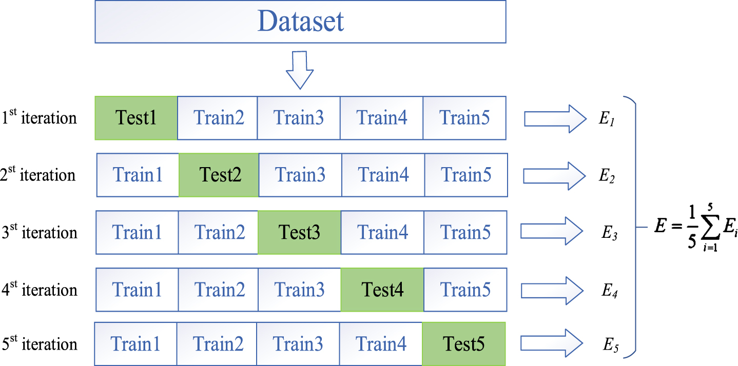
Data set partitioning at K = 5.

When using K-fold validation, the same parameters are set up as in the ablation experiment, and the comparison test is trained to ensure the accuracy of the results. The results obtained from training are divided into two parts: one for the training set results and one for the test set results. Each fold is trained for 300 rounds, and the result of the epoch with the highest accuracy of the test set in each fold is taken for the final average calculation. Table 3 shows the training results obtained by performing K-fold validation on the original model and the improved model. From the training results, it can be seen that the original network training results are still unstable under different divisions and the training results have a wide range of differences. The improved network training did not show significant differences in the training results for each fold, and compared with the results obtained from random partition validation, it was more accurate and stable, indicating that the improved network was more accurate and stable.

Table 4

Results of 5-fold validation

Model	Train accuracy/%	Test accuracy/%
SSD	87.87	87.00
	86.50	82.00
	84.00	90.00
	80.50	81.00
	84.12	83.50
Average	84.60	84.70
Improved SSD	88.42	91.12
	86.53	89.25
	86.95	90.13
	87.50	89.48
	87.13	89.48
Average	87.31	89.63

6 Conclusion

This article proposes a flame detection model based on an improved SSD algorithm to address the issues of inaccurate flame detection algorithms and high missed detection rates in real scenes. Resnet-50-SPD network is used as the backbone network of SSD model to screen high-quality information and improve the feature extraction capability of the model. In order to increase the contextual semantic information in the feature layer and improve the detection ability of small targets, feature fusion has been introduced. The AAM module is used to process the information carried by the feature layer before entering the prediction, which can effectively alleviate the loss of feature information caused by a decrease in the number of channels. The experimental results show that the detection accuracy of the improved SSD algorithm in this paper reaches 87.89% and 89.63% respectively on the randomly divided dataset and K-fold validation dataset, indicating that the improved algorithm can effectively solve the problems of small scale and multiple targets of flame targets. The effectiveness of the improved SSD method was verified by comparing it with classical detection algorithms. At the same time, the detection accuracy of this algorithm has greatly improved, which is conducive to promoting intelligent real-time detection of flames in actual scenes and is crucial for fire safety.

In the future, we will continue to filter and update images on existing datasets, striving to solve the problem of overfitting. On the basis of existing work, we will continue to optimize and improve the network structure to achieve better detection performance and faster detection speed. In addition, a hardware platform has been built to combine algorithms with hardware devices, improving practicality.

Footnotes

Acknowledgment

This paper was supported by (1) Youth Science Foundation of Natural Science Foundation of Henan Province (212300410185); (2) Key Scientific Research Project of Henan Province (21A510005).

References

Deng

, Beng

, Satheesh

, Su

, Khosla

and Fei-Fei

, ILSVRC-2012, 2012. URL https://www.image-net.org/challenges/LSVRC/2012/.

Redmon

, Divvala

, Girshick

et al. You only look once: Unified, real-time object detection, Proceedings of the IEEE Conference on Computer Vision and Pattern Recognition (2016), 779–788.

Liu

, Anguelov

, Erhan

et al. SSD: Single Shot MultiBox Detector[J], arXiv preprint arXiv: 1512.02325, 2015.

Girshick

, Donahue

, Darrell

et al. Rich feature hierarchies for accurate object detection and semantic segmentation, Proceedings of the IEEE Conference on Computer Vision and Pattern Recognition (2014), 580–587.

Girshick

, Fast r-cnn, Proceedings of the IEEE International Conference on Computer Vision (2015), 1440–1448.

Ren

, He

, Girshick

et al. Faster r-cnn: Towards real-time object detection with region proposal networks[J], Advances in Neural Information Processing Systems (2015), 28.

Frizzi

, Kaabi

, Bouchouicha

et al. Convolutional neural network for video fire and smoke detection, IEC-ON 2016-42nd Annual Conference of the IEEE Industrial Electronics Society (2016), 877–882.

Le Cun

Bottou

, Bengio

, et al. Gradient-based learning applied to document recognition[J], Proceedings of the IEEE 86(11) (1998), 2278–2324.

Zhang

, Xu

et al. Deep convolutional neural networks for forest fire detection, In 2016 International Forum on Management, Education and Information Technology Application (2016), 568–575.

10.

Kim

and Lee

, A video-based fire detection using deep learning models, Applied Sciences 9(14) (2019).

11.

Fang

, Wang

and Ren

, Tinier-YOLO: a real-time object detection method for constrained environments[J], IEEE Access 8 (2019), 1935–1944.

12.

, Zhang

, Liu

et al. A visualized fire detection method based on convolutional neural network beyond anchor[J], Applied Intelligence (2022), 1–16.

13.

Sun

and Xin

, Flame Detection Algorithm Based on YOLOv4, Proceedings of the IEEE 7th International Conference on Intelligent Computing and Signal Processing (2022), 314–317.

14.

Bochkovskiy

, Wang

C.Y.

and Liao

H.Y.M.

, Yolov4: Optimal speed and accuracy of object detection[J], arXiv preprint arXiv:2004. 10934, 2020.

15.

, Zhang

, Ren

et al. Spatial pyramid pooling in deep convolutional networks for visual recognition[J], IEEE Transactions on Pattern Analysis and Machine Intelligence 37(9) (2015), 1904–1916.

16.

Liu

, Qi

, Qin

et al. Path aggregation network for instance segmentation, Proceedings of the IEEE Conference on Computer Vision and Pattern Recognition (2018), 8759–8768.

17.

Jeon

, Choi

H.S.

, Lee

et al. Multi-scale prediction for fire detection using convolutional neural network, Fire Technology (2021), 57.

18.

, Xue

and Li

, Real-Time Video Fire Detection via Modified YOLOv5 Network Model[J], Fire Technology (2022), 1–27.

19.

Qin

Y.Y.

, Cao

and Ji

X.F.

, Fire detection method based on depthwise separable convolution and YOLOv3[J], International Journal of Automation and Computing 18(2) (2021), 300–310.

20.

, Lin

, Lu

et al. A Forest Fire Detection System Based on Ensemble Learning[J], Forests 12(2) (2021), 217.

21.

Majid

, Alenezi

, Masood

et al. Attention based CNN model for fire detection and localization in real-world images, Expert Systems with Applications (2022), 189.

22.

Sunkara

and Luo

, No more strided convolutions or pooling: a new CNN building block for low-resolution images and small objects, Machine Learning and Knowledge Discovery in Databases: European Conference (2022), 443–459.

23.

Shrivastava

, Gupta

and Girshick

, Training region-based object detectors with online hard example mining, IEEE Conference on Computer Vision and Pattern Recognition (2016), 761–769.

24.

Wang

, Chen

, Dong

et al. Improved YOLOv5 network for real-time multi-scale traffic sign detection[J], Neural Computing and Applications (2022), 1–13.

25.

Neubeck

and Van

, Gool, Efficient Non-Maximum Suppression. 18th International Conference on Pattern Recognition (ICPR’06), IEEE (2006), 850–855.

26.

, Jiang

, Wang

et al. UnitBox: An advanced object detection network, Proceedings of the 24th ACM International Conference on Multimedia (2016), 516–520.

27.

, Zhang

, Ren

et al. Deep residual learning for image recognition, Proceedings of the IEEE Conference on Computer Vision and Pattern Recognition (2016), 770–778.

28.

Jin

, Fu

, Wang

et al. Multi-feature fusion and enhancement single shot detector for traffic sign recognition[J], IEEE Access 8 (2020), 38931–38940.

29.

Ioffe

and Szegedy

, Batch normalization: Accelerating deep network training by reducing internal covariate shift, International Conference on Machine Learning (2015), 448–456.

30.

Foggia

, Saggese

and Vento

, Real-time fire detection for video-surveillance applications using a combination of experts based on color, shape, and motion, IEEE Transactions on Circuits and Systems for Video Technology 25(9) (2015), 1545–1556.

31.

Redmon

and Farhadi

, Yolov3: An incremental improvement[J], arXiv preprint arXiv:1804.02767, 2018.

32.

C.Y.

, Liu

, Ranga

et al. DSSD: Deconvolutional single shot detector[J], {arXiv preprint arXiv:1701.06659, 2017.

Research on flame detection method based on improved SSD algorithm

Abstract

Keywords

1 Introduction

2 SSD target detection algorithm

Table 1 ResNet50-SPD architecture Layer name ResNet-50-SPD Spd1 SPD-Conv Conv1 3 × 3, 64 Conv2-x [ 1 × 1 , 64 3 × 3 , 64 1 × 1 , 256 ] × 3 Spd2 SPD-Conv Conv3-x [ 1 × 1 , 128 3 × 3 , 128 1 × 1 , 512 ] × 4 Spd3 SPD-Conv Con4-x [ 1 × 1 , 256 3 × 3 , 256 1 × 1 , 1024 ] × 6 Spd4 SPD-Conv

4.1 Image dataset

4.3 Training parameters

4.4 Evaluation indicators

5.1 Analysis of training results

Table 2 Results of ablation experiment Experiment VGG ResNet-50-SPD Feature fusion AAM mAP/% FPS/f/s 1 √ 83.92 65.6 2 √ 84.36 65.1 3 √ √ 85.12 64.6 4 √ √ 86.27 64.1 5 √ √ √ 87.89 62.9

Table 3 Performance comparison of different algorithms Model mAP/% FPS YOLOv3 83.51 54.6 YOLOv4 84.26 56 YOLOv5s 86.91 67.1 Faster R-CNN 83.66 23.6 SSD 83.92 65.6 D-SSD 86.78 49.5 Improved SSD 87.89 64.9

Footnotes

Acknowledgment

References

Table 2
Results of ablation experiment

Experiment VGG ResNet-50-SPD Feature fusion AAM mAP/% FPS/f/s

1 √ 83.92 65.6

2 √ 84.36 65.1

3 √ √ 85.12 64.6

4 √ √ 86.27 64.1

5 √ √ √ 87.89 62.9

Table 3
Performance comparison of different algorithms

Model mAP/% FPS

YOLOv3 83.51 54.6

YOLOv4 84.26 56

YOLOv5s 86.91 67.1

Faster R-CNN 83.66 23.6

SSD 83.92 65.6

D-SSD 86.78 49.5

Improved SSD 87.89 64.9