A novel ensemble learning approach for fault detection of sensor data in cyber-physical system

Abstract

Cyber-physical systems (CPS) play a pivotal role in various critical applications, ranging from industrial automation to healthcare monitoring. Ensuring the reliability and accuracy of sensor data within these systems is of paramount importance. This research paper presents a novel approach for enhancing fault detection in sensor data within a cyber-physical system through the integration of machine learning algorithms. Specifically, a hybrid ensemble methodology is proposed, combining the strengths of AdaBoost and Random Forest with Rocchio’s algorithm, to achieve robust and accurate fault detection. The proposed approach operates in two phases. In the first phase, AdaBoost and Random Forest classifiers are trained on a diverse dataset containing normal and faulty sensor data to develop individual base models. AdaBoost emphasizes misclassified instances, while Random Forest focuses on capturing complex interactions within the data. In the second phase, the outputs of these base models are fused using Rocchio’s algorithm, which exploits the similarities between faulty instances to improve fault detection accuracy. Comparative analyses are conducted against individual classifiers and other ensemble methods to validate the effectiveness of the hybrid approach. The results demonstrate that the proposed approach achieves superior fault detection rates. Additionally, the integration of Rocchio’s algorithm significantly contributes to the refinement of the fault detection process, effectively leveraging the strengths of AdaBoost and Random Forest. In conclusion, this research offers a comprehensive solution to enhance fault detection capabilities in cyber-physical systems by introducing a novel ensemble framework. By synergistically combining AdaBoost, Random Forest, and Rocchio’s algorithm, the proposed methodology provides a robust mechanism for accurately identifying sensor data anomalies, thus bolstering the reliability and performance of cyber-physical systems across a multitude of critical applications.

Keywords

Cyber-physical systems fault detection sensor data ensemble learning random forest

1 Introduction

In the realm of contemporary technological advancements, the pivotal role of cyber-physical systems (CPS) and sensor networks [1, 2] in critical applications cannot be overstated. From industrial automation to healthcare monitoring, these interconnected systems underpin a wide array of essential functions. One of the linchpins of their operation is the reliability and accuracy of sensor data, which forms the foundation for informed decision-making and optimal system performance within these networks. Ensuring the integrity of this sensor data is imperative to prevent cascading failures and maintain the desired functionality. In this context, this research paper introduces a pioneering approach aimed at elevating the efficacy of fault detection within sensor data of cyber-physical systems. This is accomplished through the strategic integration of advanced machine learning algorithms, forging a path toward heightened system resilience and precision. The procedure of fusing the forecast outcomes provided by the multiple ML algorithms lowers the probability of selecting the wrong models by a large margin [3].

The CPS takes a coordinated approach to the management of communication networks, computer resources, controllers, and physical surroundings. For the purpose of keeping monitors on the physical phenomena that will impact the calculations, it is outfitted with a network of embedded computers. In such an environment, cyber-attacks may generate significant threats to the systems that are under the surface [4, 5]. When it comes to the design of CPS security, the standard techniques treat the physical and cyber systems in isolation. This renders them defenceless against threats posed by Networks and embedded controllers are used to observing and manage physical processes [6, 7]. As a consequence of this, an integrated security strategy is required to defend CPS against cyberattacks.

The central proposition of this paper revolves around the development of a hybrid ensemble methodology, meticulously crafted to harness the strengths of three distinct algorithms: AdaBoost, Random Forest, and Rocchio’s algorithm. This fusion is designed to overcome the limitations of individual techniques and capitalize on their collective potential to achieve a fault detection mechanism that is robust, adaptable, and accurate. The proposed methodology unfolds in two distinct but synergistic phases, each playing a pivotal role in the overall enhancement of fault detection.

In the initial phase, AdaBoost and Random Forest classifiers are meticulously trained using a diverse dataset comprising both normal and faulty sensor data. This foundational training lays the groundwork for the subsequent phases and equips the classifiers to recognize intricate patterns within the data. AdaBoost, with its emphasis on addressing misclassifications, and Random Forest, with its capacity to capture complex relationships, contribute unique dimensions to the methodology. The second phase entails the orchestration of these base classifiers through Rocchio’s algorithm, a mechanism designed to capitalize on the shared traits of faulty instances and further refine the fault detection process. By tapping into the similarities that often exist between instances of malfunction, Rocchio’s algorithm serves as a potent tool in elevating the accuracy of the fault detection process. Comparative evaluations are conducted to establish the efficacy of this hybrid ensemble approach, both against individual classifiers and alternative ensemble strategies, validating its superior performance.

In summation, this research embodies a comprehensive and innovative solution aimed at fortifying the fault detection capabilities of cyber-physical systems. The harmonious integration of AdaBoost, Random Forest, and Rocchio’s algorithm unfolds new vistas in fault detection, enabling these systems to accurately identify anomalies within sensor data. By enhancing the reliability and precision of cyber-physical systems across diverse critical applications, this research offers a compelling contribution to the domain of modern technology and its intersection with vital real-world functions.

CPSs may perceive actions of physical occurrences and communicate with a set of systems through the Internet [8, 9]. Additionally, it has the capacity to adjust to changes in its environment, which is very useful in CPS applications that make use of several network nodes. Additionally, there is a greater possibility of difficulty when gaining access to any channel. As was indicated, the CPS functions as a regulatory system over connected computers, and it is responsible for transmitting instructions for a variety of tasks. As a direct consequence of this, the CPS receives feedback in the form of results about the operation of various processes. In order to automate the operations that are carried out in a variety of control and design domains, cyber physical systems are used [10]. CPS is most often used in medical departments and army domains for the purpose of offering automated procedure in situations when humans are unable to operate successfully [11]. CPS is believed to be vital since it contains sensor and actuator devices in home-based, medical and transport applications [12 –14].

The need for a novel fault detection algorithm for sensor data in cyber-physical systems is driven by the increasing complexity and interconnectedness of these systems. CPS are often used in critical applications, such as power grids, transportation systems, and healthcare. Faults in CPS can have serious consequences, such as power outages, transportation accidents, and patient harm. Traditional fault detection algorithms are often not effective in detecting faults in CPS. This is because CPS data can be noisy, contain outliers, and be subject to adversarial attacks. Novel fault detection algorithms are needed that can address these challenges and ensure the reliability of CPS. The process of fault detection has to be accurate and quick in order to prevent any kind of loss. For example, it needs in order to limit loss in the system, it is necessary to be able to distinguish between abnormal and typical settings. the event that incorrect data is acquired, which might result in inaccurate conclusions. by integrating the M models into an ensemble model, $ψ φ_{Lk}^{1}, φ_{Lk}^{2} \dots φ_{Lk}^{M}$ the ensemble algorithm makes its ultimate conclusion. The ensembles are combined using the majority-vote method for zero-one classification, as stated in Equation (1). $ψ_{Lk} (x) = ψ φ_{Lk}^{1}, φ_{Lk}^{2} . φ_{Lk}^{M (x)} = {c ɛ y}_{arg \max} \sum_{m = 1}^{M} (φ_{Lk}^{m} (x) = c)$ (1)

1.1 Faults in sensor data

The data-centric view of sensor networks is where these faults are located, whereas the system-centric perspective is where calibration failures and battery failures are gathered together. As a result of the harsh and hostile environments in which sensor networks are often deployed, such as during a thunderstorm, a snowfall, or heavy rain, it is quite possible that they will make mistakes both frequently and unexpectedly. The emergence of defects during normal operation may have severe repercussions, involving economic loss, environmental harm, and loss of human life. These outcomes can be caused by a variety of factors. Faults are separated into their respective classifications so that catastrophic outcomes like these may be avoided. The following provides, in accordance with the data that was gathered, a description of the various kinds of defects [15].

The data that were collected are modelled using the triplet d (n, t, f (t)) ; where f(t) represents the perceived value that node n had at time t. The representation of this equation is shown in Equation (2):

$f (t) = α + β x + η$ (2)

In the above equation, “sensed data f(t) is modelled as α, which is offset, β represents gain, and while η is the noise present in the data.”

Gain Faults

The term “gain fault” refers to a situation in which the rate of change in the data is greater than the reading that was anticipated. This occurs due to the multiplicative nature β of the relationship between and the data point x. Equation (3) is a representation of this flaw in the system. $x^{'} = β x + η$ (3)

Where β represent the constant, “which is multiplied with the normal reading.”

Offset Fault

An offset problem occurs when the data that have been gathered are not in line. This occurs as a result of erroneous calibration of the sensing unit, which causes a constant to be added to the data that was anticipated. The following is one way to simulate an offset fault which is represented in the Equation (4) $x^{'} = α + x + η$ (4)

Where α represent the constant value added in the normal reading.

Stuck-at fault

Data values that remain constant or nearly constant for longer than intended constitute a stuck-at fault. Equally opposed to the result one would anticipate from these phenomena, the zero variation must occur. Using Equation (5), the model is presented as:

$x^{'} = α$ (5)

Where x′ is “the non-faulty data gathered by the node at time t.”

To construct an observation vector or data sample (Xτ), four successive instances or data measurements were considered: (tn, tn + 1 … tn + N). There were two readings from the temperature (T) sensor and two readings from the humidity (H) sensor for each data point.

2 Related work

Mboweni et al. [16] examined that it is essential to keep vital infrastructure like water treatment and distribution systems secure in order to keep the economy running smoothly. Many security flaws exist in these systems because they use cyber-physical components. Intrusion detection systems are vital to ensuring network safety because they help mitigate the impact of any successful assaults. While machine learning’s pattern-analysis capabilities might improve security, some characteristics of the data may compromise the model’s accuracy. Complexity, variety, irregularity, and sensitivity make data from important water system infrastructure challenging to deal with. Changes in the environment and adjustments to operations might cause the measurements to fluctuate over time, which is reflected in the data. To deal with the complications and guarantee reliable analysis, efficient data pretreatment methods are required to manage irregular patterns and tiny changes. Using a dataset from a water treatment plant as a case study, this article delves into the topic of data preparation and proposes methods tailored to the processing of data in industrial control.

Mall et al. [17] stated that the prevalence of Distributed Denial of Service (DDoS) assaults has grown steadily. As a result, genuine users can’t use the service, and the network’s overall performance suffers. When computing, networking, and physical factors are brought together, a CPS is produced. An up-and-coming design, Software-Defined Networking (SDN) separates networking tasks from data processing. SDN is susceptible to DDoS attacks because its control logic is located in the control plane. With the help of deep learning, many AI applications and services can carry out cognitive activities normally requiring human interaction, greatly increasing the efficiency of automation. This study introduces many Using a flexible and adaptable Deep Learning framework, the SD-CPS framework can detect DDoS attacks. scalable software-defined network (SDN) architecture.

Kandasamy et al. [18] studied that the development of embedded systems and WSNs has made possible low-cost monitoring and automation options for smart grids. A “smart grid” is a network of subsystems and metasystems that is supposed to make the traditional electricity grid more efficient and reliable. For a smart grid to be effective, it must be able to exchange information back and forth between power companies and consumers. This study suggests a new approach to improving smart grid security and defect detection in the industrial sector by combining a WSN with deep learning architectures. Since security is the primary hindrance to smart grid adoption, the suggested paradigm is useful for smart grid operations in order to boost security and industrial fault detection throughout the network.

Alwan et al. [19] analyzed that in large-scale CPSs, sensor node failures are unavoidable and unforeseen occurrences that may threaten the accuracy of sensor data, the efficacy of CPS services, and the safety, dependability, performance, and security of the system as a whole. While numerous papers have proposed domain-specific solutions to the problem of detecting failed sensor nodes, this one presents a fresh approach to the problem and uses a case study to experimentally test its viability. In this research, the application of time-series clustering algorithms as a realistic method for identifying faulty sensor nodes by identifying long-segmental outliers in the time series of the observations is investigated. This research shows that time-series clustering may be used to efficiently identify both continuous (halting/repeating) and early-stage problems in a sensor node. Feature-based time series clustering outperforms shape-based time series clustering when used with shorter time-series frames. approaches like DTW and K-Shape in finding long-segmental outliers.

Wardhani et al. [20] intended that WSNs are a highly diversified cyber-physical system, making them susceptible to a wide range of failures that might have far-reaching effects on security, the economy, and reliability. Fault identification and diagnosis in Due to the vast range of installations and the constrained capabilities of available sensor resources, WSNs is a challenging problem. A strategy based on supervised machine learning is employed in this investigation. SVM and Random Forest (RF) are two of the most cutting-edge ML algorithms, and they are used to evaluate how well the suggested scheme performs in comparison. The findings of this research indicated that machine learning models built to foresee defects in WSN data obtained using the RUS sampling approach might be affected both favorably and adversely by this choice.

Mittal et al. [21] suggested that the usage of various networks to transport data by the Industrial IoT creates many cyber-physical attacks. Data security is further complicated by the absence of labels. This study introduces a novel clustering approach for detecting intrusions. To acquire the best clusters, the suggested technique uses a new twist on the gravitational search algorithm. The suggested alternative makes use of a logistic-mapping-based chaotic function with an exponentially diminishing K best. Maximum improvements in all dimensions were seen with the suggested version.

Tavolato et al. [22] proposed an innovative method for modelling extremely complex systems with many sensors, actuators, and controllers in order to find abnormalities in cyber-physical systems. Our strategy is based on the analytical methods frequently employed in kinetic gas theory, which aims to characterize a gas’ overall behaviour without taking individual molecules into account. The hypotheses is formulated about the system’s overall behaviour by modelling it as a multi-agent network. The system’s performance may be tracked using these forecasts. The monitoring system may sound an alert if there is a significant discrepancy between forecasted and real values for the properties of a cyber-physical system. This method of anticipating a cyber-physical system’s typical behaviour is based on the system’s definition and intended use, as opposed to the more prevalent machine learning methods, which depend on the actual performance throughout a training phase, of the system.

Yang et al. [23] studied that energy systems may be made more reliable and cost-effective during their lifetimes if they are operated as efficiently as possible. Intelligent use of large data acquired during operation or forecast is required to determine effective operating strategies. As a result, it is becoming more common to use CPS to integrate large data with physical models in order to obtain highly-reliable and -accurate predictions. A methodology for systematically using CPS in thermal power plant performance analysis and decision making is provided. An overall CPS technique for use in thermal power plants, including both offline and online phases, and spoke about the various ways used to back up these individual steps is offered. Each physical component is modelled and linked together using operational history data collected and stored in the cyber layer. Online usability is further shown by providing an example of the decision-making process involved in determining the best frequency of air-cooling condenser operation. The combination of the cyber-physical system and the data mining approach is shown to be efficient and holds great promise for improving the management and analysis of thermal power plants in real time.

3 Proposed approach

This section explains our proposed method for an ensemble random forest that looks for faults in a network. The fundamental concept behind the ensemble learning model is to first build many instances of the base model u, and then to integrate the outcomes of these instances using the Equation (1). When compared to a single classifier, the results produced by a combination of many classifiers are superior. As a foundational learning model for our study, three different classifiers are used: Naive Bayes, K-Nearest Neighbors, and Support Vector Machines (SVM). The ensemble learning model is used to train each bootstrap sample that is generated. After that, the aggregated results of several base learning models are used to make the final determination.

3.1 Feature selection (CMI)

It is extremely uncommon for all of the variables in a dataset to be significant when using machine learning in the actual world to build a model. This is because there are so many different factors that may influence the outcome of the process. As a consequence of the inclusion of redundant variables, the ability of the model to generalize is reduced, which may also lead to a decline in the overall accuracy of the classifier. In addition to this, the incorporation of more variables into a model will lead to an increase in that model’s overall level of complexity. The primary goal of feature selection strategies in machine learning is to identify the optimal set of features that will construct practical models reflecting the phenomenon being studied. Conditional Mutual Information [24] serves as the cornerstone of this phase in our strategy, serving to provide insights into the specific flaws that warrant investigation and detection. By utilizing this technique, the streamline data processing for fault detection within sensor data is endeavored, effectively identifying and isolating the most pertinent features that significantly impact the targeted outcomes.

Conditional Mutual Information

The normal operating conditions is also considered as a parameter, any data points that fall outside of this range are considered as anomalies, and could be indicative of a fault. Considering X, Y and Z as the parameters of the dataset, the accuracy of fault detection systems can be improved as these parameters provide information about the expected behaviour of the system, which can be used to identify anomalies that may indicate a fault. The features with the highest CMI values would be the most relevant for fault detection, meaning these two features are highly correlated and provide complementary information about the state of the sensor network and could be used to develop a fault detection system as mentioned in Equation (6). $I (X; Y | Z) = H (X | Z) - H (X | Y, Z)$ (6)

Where H (X|Z) is the entropy of X given Z, and H (X|Y, Z) is the entropy of X given Y and Z.

The entropy of a random variable X is defined in Equation (7) $H (X) = - \sum_{x} p (x) {log}_{2} p (x)$ (7)

Where p (x) is the probability that X takes on the value x.

The entropy quantifies the degree to which X is likely to surprise us. Furthermore, H (X) is roughly equivalent to the average amount of knowledge gained from a single occurrence of the random variables X. It’s vital to keep conscious that the algorithm’s base is irrelevant since the values of the entropy only vary when the base is changed by a multiplicative constant.

The joint entropy measures the degree of uncertainty in the two random variables, X and Y, when they are combined.

Given Y, the conditional entropy of X is mentioned in the Equation (8) $H (X | Y) = \sum_{y} p (y) \sum_{x} p (x ∣ y) {log}_{2} p (x ∣ y)$ (8)

Where p (x ∣ y) is the probability that X takes on the value x given that Y takes on the value y. The conditional entropy measures the amount of remaining uncertainty as the value of another random variable, Y, but not X is known.

Mutual Information: According to p (x, y), the mutual information between two discrete random variables X, Y is provided by in Equation (9) which can be used to analyze the similarity of two sets of data and the predictability of the system. $\begin{matrix} I (X; Y) = Xx, yp (x, y) loglogp (x, y) p (x) p (y) \\ = H (X) - H (Y) \\ = H (Y) - H (Y | X) \\ = H (X) + H (Y) - H (X, Y) \end{matrix}$ (9)

The conditional mutual information for the dataset containing faults is graphically represented in Fig. 1. The figure shows the relationship between the features and can be used to identify which features are most important for predicting the target variable. This information can be used to improve the accuracy of the proposed algorithm by reducing the number of features and ensuring that the most important features are selected.

Fig. 1

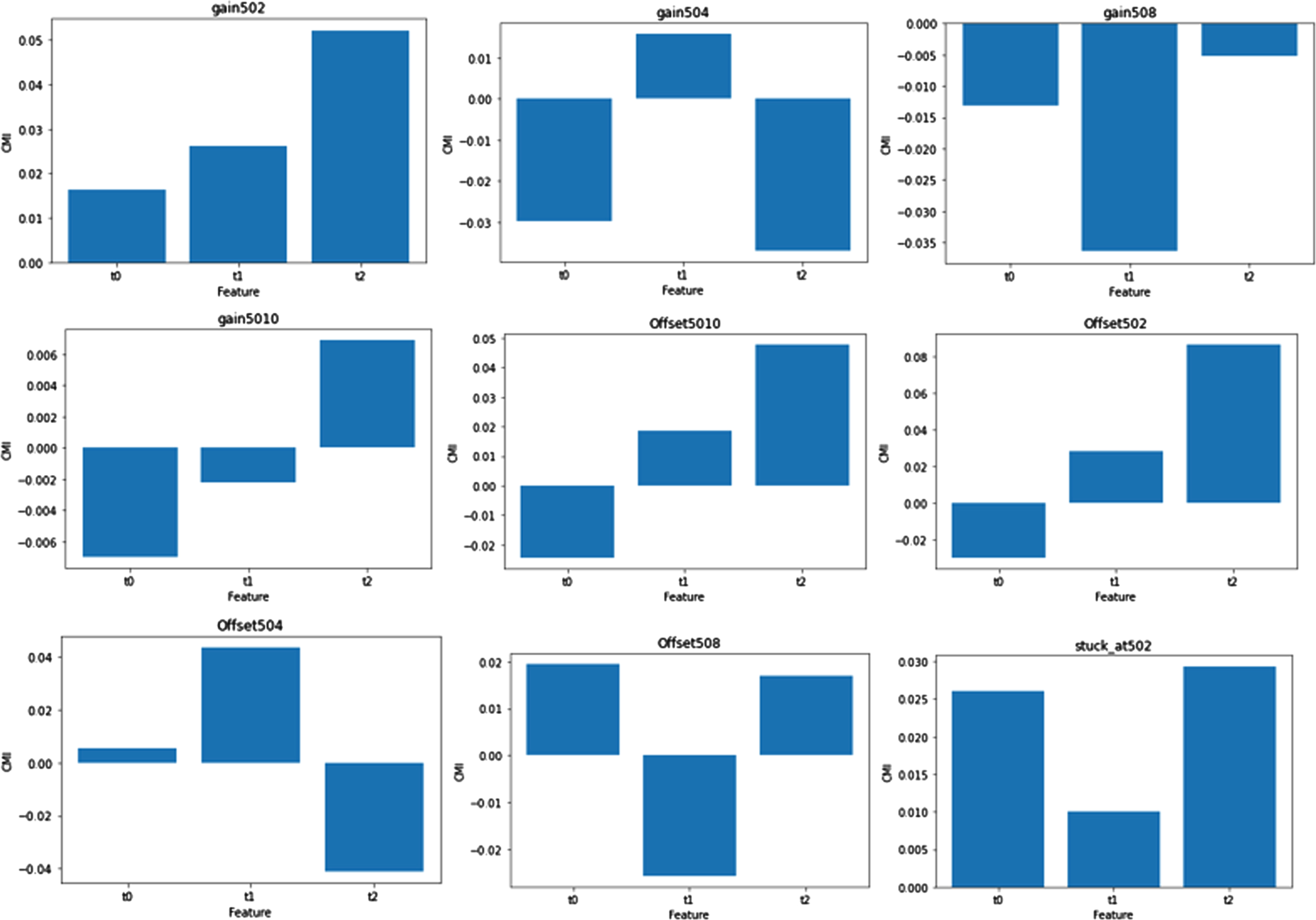
Conditional mutual information for the fault dataset.

3.2 Model construction

The proposed approach shows the use of the CMI feature selection method to select features for fault detection in WSNs. CMI is a more principled approach than traditional feature selection methods, and it has been shown to improve the accuracy of the fault detection process. In addition, it uses a hybrid ensemble of classifiers, which is more robust to noise and outliers than a single classifier. This further improves the accuracy of the fault detection process. The detailed model is shown in the Fig. 2.

Proposed Framework:

Fig. 2

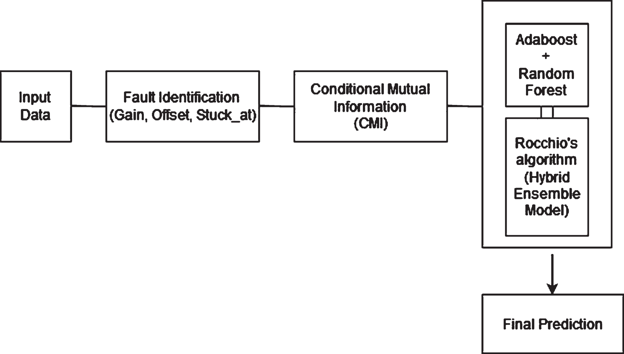
Hybrid ensemble model framework

Data Preparation: The detected interpretation is forwarded to the data preparation block, where each data measurement Vt is used to generate a new observation vector. The observation vector Vt comprises humidity measures H1, H2, and temperature observations T1, T2. To generate a new observation vector, data measurements Vt, Vt-1, and Vt-2 are aggregated.

Fault Injection: After observation vector generation, faults are introduced into the dataset. Faults, such as gain, stuck-at, and offset, are inserted according to the second development stage of the system model, using datasets with pre-existing flaws from acquired data.

Feature Selection Using Conditional Mutual Information (CMI): The Conditional Mutual Information (CMI) feature selection method is used in the data processing pipeline. CMI helps identify significant features by measuring the relationships between variables while accounting for the presence of other variables. This step aids in reducing redundancy and enhancing the model’s ability to generalize, thus contributing to more accurate fault detection.

Ensemble Learning for Enhanced Fault Detection: Following the application of CMI feature selection, the ensemble learning approach combines the outputs of AdaBoost and Random Forest classifiers [25] using Rocchio’s algorithm. The combination of AdaBoost, random forest, and Rocchio’s algorithm can be used to detect and prevent sensor data attacks. AdaBoost can be used to identify the most important features in the sensor data. Random forest can be used to classify the data into normal and attack samples.

Conclusion: This framework outlines a comprehensive approach for fault detection of sensor data in cyber-physical systems by strategically integrating the CMI feature selection method and incorporating the provided points. This combination of techniques results in a robust and accurate fault detection framework.

3.3 Proposed algorithm

The algorithm works by first training a set of weak learners on the training data. The weak learners are then used to calculate the relevance scores and the variance for each data point in the training data. The relevance scores measure how likely a data point is to be faulty, while the variance measures how much uncertainty there is about the prediction of the weak learners for a data point.

A random forest is then trained on the training data. The random forest is used to predict the class of each data point in the training data. The predictions of the random forest are then used to calculate the weighted sum of the relevance scores, the variance, and the predictions of the random forest.

The strong learner is then updated using the weighted sum. The weights of the weak learners are then updated based on the error of the weak learners. The algorithm iterates until the error of the strong learner converges.

The AdaBoost-Random Forest-Rocchio algorithm is a powerful algorithm for fault detection in sensor data. The algorithm combines the strengths of AdaBoost, random forest with Rocchio’s algorithm [26] to achieve high accuracy and robustness in fault detection.

Algorithm: AdaBoost-Random Forest-Rocchio algorithm for fault detection in sensor data.

Given: Set D of sensor data with labels y, number of weak learners n and parameters λ and σ.

Strong learner H

Weak learner f

1. Initialize the set of weak learners F to be empty.

2. For i = 1 to n :

a. Train a weak learner f on D.

b. Add f_i to F.

3. Calculate the relevance scores R (x) for each data point x in D as follows $R (x) = \sum_{i = 1}^{n} . w_{i} . y_{i} . f_{i} (x)$

4. Calculate the variance σ² (x) for each data point x in D as follows:

$σ^{2} (x) = \sum_{i = 1}^{n} ω_{i}^{2} \cdot {(f_{i} (x) - \bar{f})}^{2}$

5. Train a random forest R on D. $f (x) = \frac{1}{T} \sum_{t = 1}^{T} f_{t} (x)$

6. Initialize the strong learner H to be the zero vector.

7. For each data point x in D:

a. Calculate the weighted sum of the relevance scores and the variance $S (x) = λ \cdot R (x) + σ (x)$

b. Calculate the weighted sum of the relevance scores, the variance, and the predictions of the random forest $T (x) = S (x) + R (x) . R (x) + σ (x) . R (x)$

c. Update the strong learner H as follows:

$H \leftarrow H + T (x) \cdot x$

8. The weights of the weak learners are then updated $ω_{i} = ω_{i} - \frac{1 - ɛ_{i}}{ɛ_{i}}$

9. Return the strong learner H.

D is the set of sensor data, F is the set of weak learners, and H is the strong learner. The goal is to find a function f : D→ { 0, 1 } that can be used to detect faults in the sensor data, where w_i is the weight of weak learner i, y_i is the label of data point x in the training set, and f_i (x) is the prediction of weak learner i for data point x.

Once the average prediction is acquired, the variance for each data point x by taking the sum of the squared differences between the predictions of the weak learners and the average prediction can be calculated. Each squared difference is weighted by the square of the ω_i value for the corresponding weak learner where f is the average of the predictions of the weak learners. The algorithm then trains random forest R on D which uses multiple decision trees to make predictions.

For each data point x in D, the algorithm calculates the weighted sum of the relevance scores and the variance where λ is a hyperparameter that controls the importance of the relevance scores and the variance. The weighted sum of the relevance scores, the variance, and the predictions of the random forest are calculated. The variance of the predictions of a decision tree is high when the decision tree is overfit to the training data. The random forest algorithm reduces the variance of the predictions by training the decision trees on different subsets of the data. The decision trees are trained on different subsets of the data, and the predictions of the decision trees are combined to make a final prediction.

The strong learner is initialized to be the zero vector. This means that the initial prediction of the strong learner is always the same, regardless of the input data. The weak learners are then trained sequentially. After each weak learner is trained, its prediction is added to the strong learner with a weight that is inversely proportional to the error of the weak learner. This process continues until the desired number of weak learners have been trained. The algorithm repeats steps 2 to 8 until the desired accuracy is achieved. The final prediction of the strong learner is the weighted sum of the predictions of the weak learners.

4 Dataset and implementation

4.1 Dataset explanation

A collection of observations with a dimension of 12 make up the dataset. Measurements are contained in each (vector) in three subsequent occurrences (t0, t1, and t2). There are two observations of temperature and two measures of humidity for each occurrence (T1 T2 and H1 H2). Hence there are 4688 observations each randomly has been introduced to faults described in the previous section. The rates of faults induced are from 10 percent to 50 percent with an incremental of 10 percent at each stage. About 60 datasets have been prepared. There are two Excel files for each dataset (one for observations and one for label y). Y is equal to 1 in normal observations and –1 in fault observations. Researchers from Qassim University in Saudi Arabia compiled a labelled dataset in 2018 that consisted of temperature and humidity readings from outside data gathering via multi-hop wireless networks. The dataset was acquired from outdoor environments. Each defect required its own unique dataset, which was then created before the fault was inserted. There are a total of 4688 samples available [27].

4.2 Implementation results

The three metrics to evaluate the effectiveness of the classifiers that are a component of the proposed strategy are accuracy, recall and precision.

Accuracy

The method of selecting the best machine learning model for a given task, often the discovery of patterns and correlations in data. This approach makes advantage of the collected training data for the machine learning model. Here, the formula is presented as an equation. $“ Accuracy = \frac{(TP + TN)}{(TP + FP + TN + FN)} "$ (10)

Precision

Performance of a machine learning model is evaluated using the measurements’ precision and predictability. The following calculation may be used to calculate the precision: Divide the total number of correct guesses by the total number of guesses to calculate the percentage of correct guesses. The following equation displays the formula. $“ Precision = \frac{Truepositive}{Truepositive + Falsepositive} "$ (11)

Recall

Total up the number of “true positives” and “accurate hits” that were found in the search results. Recall A high degree of accuracy may be defined as a high percentage of correct hits being returned, or the number of true positives. The formula is shown in the following equation. $Recall = \frac{Truepositive}{Truepositive + Falsenegative}$ (12)

ROC Curve:

The Receiver Operating Characteristics (ROC) curve shows the model’s accuracy over a variety of categorization thresholds (as determined by the true positive and false positive rates). The TPR is the proportion of positive instances that are correctly classified as positive, while the FPR is the proportion of negative instances that are incorrectly classified as positive. The area under the ROC curve (AUC) is a measure of the overall performance of the model. A higher AUC indicates a better model.

The following tables provides accuracies obtained after implementation. Following were the weak learners identified from the given datasets.

Gain502,504,506,508 and 5010.

Offset 502,504,506,508 and 5010

Stuck at 502

The accuracy both before and after the fusion method is shown in Table 2, which can be seen below. This table takes into account 11 faults, including Gain 502, Gain 504, Gain 506, and many more. According to Table 1, Gain 502 had an accuracy of 56.24% before the fusion process, but it has now acquired a far higher accuracy, which is 99.31%. Stuck at 502 achieved a low level of accuracy before the fusion, which is equal to 50, but it has achieved a high level of accuracy after the fusion, which is equal to 100, as indicated in the table below.

Table 1

Accuracy with hybrid ensemble model

S. No	Fault	Before Fusion	After Fusion
1	Gain 502	56.24	99.31
2	Gain 504	56.24	99.31
3	Gain 506	56.24	99.31
4	Gain 508	56.24	99.31
5	Gain 5010	56.24	99.31
6	Offset 502	48.59	99.21
7	Offset 504	46.60	99.21
8	Offset 506	46.60	99.31
9	Offset 508	50	99.21
10	Offset 5010	50	98.31
11	Stuck at 502	50	98.31

Table 2

Accuracy of fault identification

S. No	Fault	k-NN	Naïve Bias	SVM	Proposed Algorithm
1	Gain 502	44.1	55.5	63.9	99.31
2	Gain 504	44.1	55.8	64.2	99.31
3	Gain 506	44.1	55.7	64.2	99.31
4	Gain 508	44.3	55.8	64.1	99.31
5	Gain 5010	44.2	55.8	64.2	99.31
6	Offset 502	44.8	72.7	84.8	99.21
7	Offset 504	44.6	58.4	79.1	99.21
8	Offset 506	44.6	60.6	81.4	99.31
9	Offset 508	44.5	54.2	62.8	99.21
10	Offset 5010	44.5	54.2	62.1	98.31
11	Stuck at 502	44.6	59.6	62.9	98.31

The faults that are present in several different classification methods are outlined in Table 2, including SVM, Naive bias, and K-NN. The accuracy of the k-NN method is 44.1 at gain 502, the accuracy of the naive bias algorithm is 55.5 at the same gain, and the accuracy of the SVM is high when compared to both k-NN and the accuracy of the naive bias algorithm. However, the suggested approach has reached the greatest accuracy possible, which is 99.31 when compared to other algorithms. At offset 502, k-NN reached 44.8, while naive bias obtained 72.7. However, the proposed approach has achieved great accuracy in comparison to other algorithms at offset 502 and offset 508, as can be seen in the table below.

Performance analysis for gain 502

As shown below in Figs. 3–5 the ROC curve is shown with number of estimators equal to 10, 50 and 100 respectively. This curve is characterized in terms of both its TPR and its FPR values. In a ROC plot, the TPR and FPR serve as the x and y axes, respectively, and show how the advantages of a positive result compare to the costs of a false positive. The sensitivity vs. (1 - specificity) plot is another name for the ROC graph. The reason for this is that TPR is equivalent to sensitivity, while FPR is equivalent to specificity multiplied by one. The accuracy (99.31), recall (78.1) and precision (80.0) achieved for the ROC curve with the number of estimators 10, 50 and 100 is represented in the Table 3.

Fig. 3

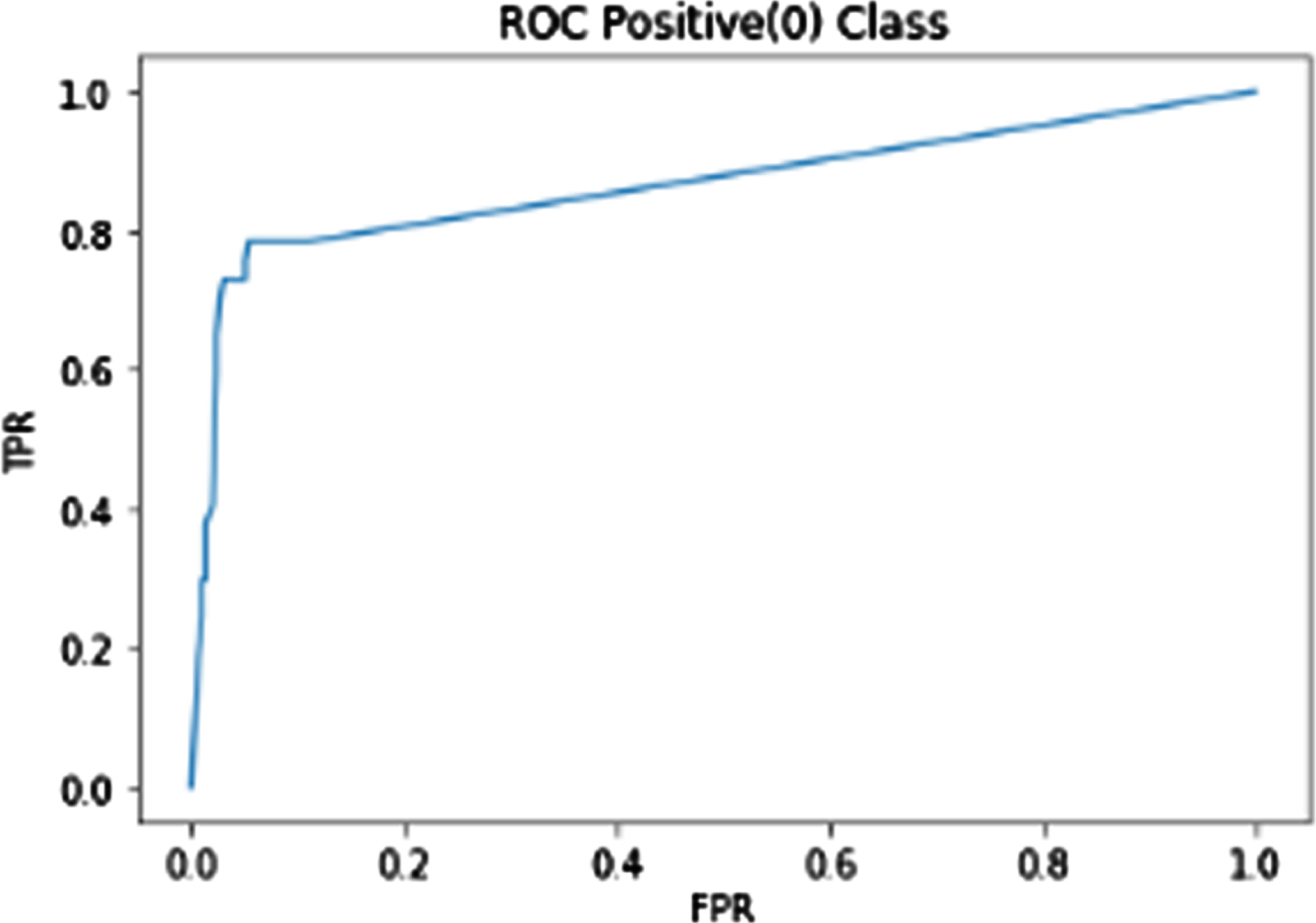
ROC curve for no. of estimators = 10.

Fig. 4

ROC curve for No. of estimators = 50.

Fig. 5

ROC curve for no. of estimators = 100.

Table 3

Accuracy, recall and precision with the number of estimators

No. of	Accuracy	Recall	Precision
estimators
10	99.31	78.1	80.0
50	99.21	76.3	78
100	98.31	77.4	80.6

4.3 Comparison

The performance analysis of suggested techniques is shown in above Table 3 as well as in Fig. 6, which can be found here. In this graph, there are several faults used in this study such as gain 502, gain 504, gain 506, gain 508, gain 5010, offset 502, offset 504, offset 506, offset 508, offset 5010 and stuck at 502 and attained accuracy at every fault. The K-NN, Naïve Bias, SVM and suggested approach are the four methods that are used. The accuracy of the support vector machine (SVM) is high when compared to both the accuracy of the k-NN technique and the accuracy of the naïve bias algorithm. The accuracy of the k-NN method is 44.1 at gain 502, while the accuracy of the naive bias algorithm is 55.5 at the same gain. In contrast to previous algorithms, the technique that was recommended has achieved the highest level of accuracy that is theoretically feasible, which is 99.31 percent. At offset 502, the k-NN algorithm achieved 99.8, while the naïve bias algorithm obtained 72.7. As shown in the comparison graph that follows, the proposed method attained to attained a level of accuracy that was superior to that of other algorithms when applied to offsets 502 and 508 and it gives outperformance as compared to other method.

Fig. 6

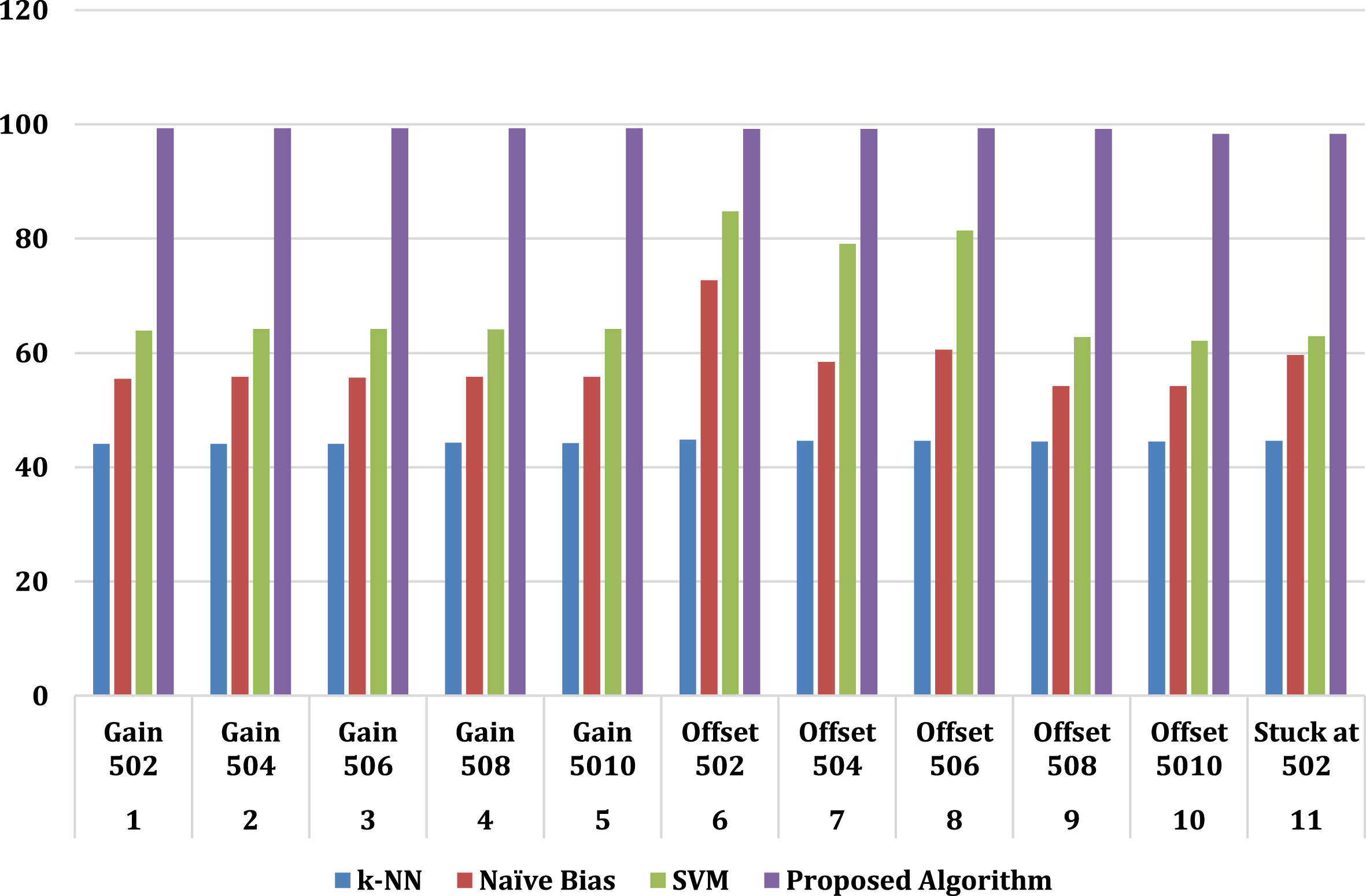
Comparison graph.

5 Conclusion and future work

In this study, a novel ensemble algorithm for trustworthiness of sensor data in cyber-physical systems using AdaBoost and random forest with Rocchio’s algorithm is proposed. The algorithm is based on the idea of combining three powerful machine learning algorithms to improve the accuracy and robustness of fault detection algorithms. The proposed algorithm on a real-world cyber-physical system dataset and compared it to several other state-of-the-art methods. The results showed that proposed method achieved the highest accuracy, precision, and recall suggesting it as a promising approach for improving the trustworthiness of sensor data in cyber-physical systems. In the future, the robustness of the proposed approach in the presence of network with a sizable number of sensors and failures will be assessed along with other type of cyber-physical systems. This research can be extended to aid cyber-attacks through anomaly detection in cyber-physical systems

References

Warriach

E.U.

, Tei

, Fault detection in wireless sensor networks: A machine learning approach, In 2013 IEEE 16th International Conference on Computational Science and Engineering, IEEE, 2013, pp. 758–765.

Muhammed

and Shaikh

R.A.

, An analysis of fault detection strategies in wireless sensor networks, Journal of Network and Computer Applications 78 (2017), 267–287.

El Hindi

, AlSalman

, Qasem

and Ahmadi

S.A.

, Building an ensemble of fine-tuned naive Bayesian classifiers for text classification, Entropy 20(11) (2018), 857.

Vinayakumar

, Alazab

, Soman

K.P.

, Poornachandran

, Al-Nemrat

and Venkatraman

, Deep learning approach for intelligent intrusion detection system, Ieee Access 7 (2019), 41525–41550.

Ding

, Han

Q.-L.

, Xiang

, Ge

and Zhang

X.-M.

, A survey on security control and attack detection for industrial cyber-physical systems, Neurocomputing 275 (2018), 1674–1683.

Tantawy

, Abdelwahed

, Erradi

and Shaban

, Model-based risk assessment for cyber physical systems security, , Computers & Security 96 (2020), 101864.

Guan

, Yang

, Chen

, Dai

and Wang

, A comprehensive overview of cyber-physical systems: From perspective of feedback system, IEEE/CAA Journal of Automatica Sinica 3(1) (2016), 1–14.

Alguliyev

, Imamverdiyev

and Sukhostat

, Cyber-physical systems and their security issues, Computers in Industry 100 (2018), 212–223.

Sztipanovits

, Koutsoukos

, Karsai

, Kottenstette

, Antsaklis

, Gupta

, Goodwine

, Baras

and Wang

, Toward a science of cyber–physical system integration, Proceedings of the IEEE 100(1) (2011), 29–44.

10.

Shi

, Wan

, Yan

, Suo

, A survey of cyberphysical systems, In 2011 International Conference on Wireless Communications and Signal Processing (WCSP), IEEE, 2011, pp. 1–6.

11.

Gunes

, Peter

, Givargis

and Vahid

, A survey on concepts, applications, and challenges in cyber-physical systems, KSII Transactions on Internet and Information Systems (TIIS) 8(12) (2014), 4242–4268.

12.

Jalandhar

D.A.V.I.E.T.

and DAVIET Jalandhar

ECE

, Impact on power consumption of zigbee based home automation network using various traffic, International Journal of Future Generation Communication and Networking 6(6) (2013), 17–24.

13.

Rajkumar

, Lee

, Sha

, Stankovic

, Cyber-physical systems: The next computing revolution, In Proceedings of the 47th Design Automation Conference, 2010, pp. 731–736.

14.

Dey

, Ashour

A.S.

, Shi

, Fong

S.J.

and Tavares

J.M.R.S.

, Medical cyber-physical systems: A survey, Journal of Medical Systems 42 (2018), 1–13.

15.

Zidi

, Moulahi

and Alaya

, Fault detection in wireless sensor networks through SVM classifier, in IEEE Sensors Journal 18(1) (2018), 340–347. doi: 10.1109/JSEN.2017.2771226.

16.

Mboweni

I.V.

, Ramotsoela

D.T.

and Abu-Mahfouz

A.M.

, Hydraulic data preprocessing for machine learning-based intrusion detection in cyber-physical systems, Mathematics 11(8) (2023), 1846.

17.

Mall

, Abhishek

, Manimurugan

, Shankar

and Kumar

, Stacking ensemble approach for DDoS attack detection in software-defined cyber–physical systems, Computers and Electrical Engineering 107 (2023), 108635.

18.

Kandasamy

, Anto

, Baranitharan

, Rastogi

, Satwik

and Sampathkumar

, Smart grid security based on blockchain with industrial fault detection using wireless sensor network and deep learning techniques, Journal of Sensors 2023 (2023).

19.

Alwan

A.A.

, Brimicombe

A.J.

, Ciupala

M.A.

, Ghorashi

S.A.

, Baravalle

and Falcarin

, Time-series clustering for sensor fault detection in large-scale Cyber–Physical Systems, Computer Networks 218 (2022), 109384.

20.

Wardhani

L.K.

, Febriyanto

R.A.

, Anggraini

, Fault Detection in Wireless Sensor Networks Data Using Ran- dom Under Sampling and Extra-Tree Algorithm, In 2022 10th International Conference on Cyber and IT Service Management (CITSM), IEEE, 2022, pp. 1–6.

21.

Mittal

, Tripathi

A.K.

, Pandey

A.C.

, Alshehri

M.D.

, Saraswat

and Pal

, A new intrusion detection method for cyber–physical system in emerging industrial IoT, Computer Communications 190 (2022), 24–35.

22.

Tavolato

, Schölnast

and Tavolato-Wötzl

, Analytical modelling of cyber-physical systems: Applying kinetic gas theory to anomaly detection in networks, Journal of Computer Virology and Hacking Techniques 16(1) (2020), 93–101.

23.

Yang

, Li

, Yang

, Wei

, Wang

and Wang

, The application of cyber physical system for thermal power plants: Data-driven modeling, Energies 11(4) (2018), 690.

24.

Zhou

H.F.

, Zhang

Y.J.

and Liu

H.J.

, Feature selection based on conditional mutual information: Minimum conditional relevance and minimum conditional redundancy, Applied Intelligence 49 (2019), 883–896.

25.

Leshem

and Ritov

, Traffic flow prediction using adaboost algorithm with random forests as a weak learner, International Journal of Mathematical and Computational Sciences 1(1) (2007), 1–6.

26.

Rocchio

J.J.

Jr , Relevance feedback in information retrieval, The SMART Retrieval System: Experiments in Automatic Document Processing (1971).

27.

Dataset reference. https://github.com/tmoulahi/Dataset-for-WSN-fault-detection