
Abstract
For solving the distributed assembly flow shop scheduling problem with fuzzy processing time (FDAPFSP), a regional biogeography-based optimization algorithm (RBBO) is proposed to minimize the maximum fuzzy completion time. The mathematical model is provided. In RBBO, all habitats are divided into regions based on the habitat suitability index, and the habitats of each region are subject to cross-regional migration and replacement procedures. A critical factory optimization strategy is developed to enhance local search capability. Taguchi method is used to determine the parameters of RBBO. In ten FDAPFSP instances, comparative testing of RBBO algorithm with various heuristic and swarm intelligence algorithms are conducted. The computation results show that in ten FDAPFSP cases, the proposed RBBO outperforms other algorithms in nine out of ten FDAPFSP cases.
Keywords
Introduction
Distributed permutation flow-shop scheduling problem (DPFSP) was first proposed by Naderi and Ruiz and had extensive research in operations research, economics, and other applications [1, 2]. DPFSP is a coupling between distributed manufacturing systems [3] and the permutation flow-shop scheduling problem (PFSP) [4], which has high practical research value.
In recent years, many scholars have also proposed many methods for DPFSP. Wang et al. [5] proposed an effective hybrid immune algorithm to solve DPFSP, designed feasible scheduling that converts job permutation sequence into factory dispatching and job sequencing, and proposed four local search methods and unique crossover factors. Gao et al. [6] proposed a new neighborhood generation method and an enhanced local search method applied to the Tabu search algorithm to solve the DPFSP.
The assembly flow-shop scheduling problem (AFSP) was first proposed by Lee et al. [7]. AFSP refers to the independent process of each job and sending the produced parts to the assembly shop for assembly. It is composed of a flow-shop scheduling problem (FSP) [8] and an assembly system [9]. Different job processing sequences can be generated during the assembly stage based on different product assembly tables, representing close relationships between enterprise managers and suppliers [10]. Many scholars have proposed valuable research on AFSP. Cai and Lei [11] proposed a new shuffled frog-learning algorithm with Q-learning to solve the distributed assembly hybrid flow shop scheduling problem. Niloofar et al. [12] considered a three-stage assembly flow shop scheduling problem with machine availability constraints and proposed two multi-objective meta-heuristics. Mohammad et al. [13] incorporates preventive maintenance into the two-stage assembly flow shop scheduling problem.
Distributed assembly permutation flow-shop scheduling problem (DAPFSP) is a combination of DPFSP and AFSP, the combination problem of DAPFSP was first proposed by Hatami et al. [14]. In the classical DAPFSP, some jobs are assigned to factories, and each factory has some machines to process each process of these jobs. FDAPFSP is the extension of DAPFSP. In real life, the processing time of jobs is often subject to a certain degree of uncertainty, which various errors may cause. Therefore, studying DAPFSP with fuzzy processing time constraints will solve real-world processing problems better. There are relatively few scholars studying FDAPFSP, but most scholars have considered other constraints. Hatami et al. [10] proposed a distributed assembly permutation flow shop scheduling problem with sequence-dependent setup times (DAPFSP-SDST). Yang and Xu [15] proposed a novel distributed assembly permutation flow shop scheduling problem with flexible assembly and batch delivery (DAPFSP-FABD). Wei et al. [16] proposed an energy-efficient distributed assembly blocking flow shop problem (EEDABFSP). Huang et al. [17] proposed an effective memetic algorithm to solve the distributed flow shop scheduling problem with an assembly machine. Zhang et al. [36] proposed a distributed estimation algorithm to solve DAPFSP and developed a matrix cube-based probability model with effective sampling mechanism to estimate the probability distribution of the optimal solution and conduct global exploration to find promising regions. Song et al. [37] used genetic programming (GP) as a high-level strategy set for generating heuristic sequences from predesigned low-level heuristics, thus proposing the GP-HH algorithm to solve DAPFSP- SDST.
Alfred Wallace and Charles Darwin introduced the idea of biogeography in the 19th century. Simon’s study of the theoretical underpinnings of biogeography was awarded the BBO in 2008 [18]. BBO performs well in comparison to other algorithms [19]. Based on the characteristics of the problem, Lin and Zhang [20] suggested an improved local search approach and a hybrid biogeography algorithm to solve DAPFSP. The efficacy of the BBO in DAPFSP is shown by this combined strategy. By dividing habitat regions based on BBO, RBBO speeds up the trend toward the dynamic balance of the habitat suitability index (HSI) by allowing better habitat migration. For maintain a dynamic equilibrium and ensure that there will never be a difference between regions, habitat replacement activities are conducted simultaneously within the region. However, many researchers added a wide range of constraints to DAPFSP and solved them; they did not impose limitations on fuzzy processing. In this paper, task processing and product assembly are given fuzzy constraints, and then 10 cases are tested by using RBBO. The results were compared using BBO and GA. The designed algorithm for FDAPFSP produced positive results.
The current research work of scholars is summarized, as shown in Table 1.
Literature comparison. Summary of literature, where the symbol “√” indicates that the corresponding assumptions has been considered
Literature comparison. Summary of literature, where the symbol “√” indicates that the corresponding assumptions has been considered
From Table 1, adding constraints is an increasingly popular research direction in studying distributed scheduling problems, and swarm intelligence algorithms are also gradually applied in distributed scheduling problems.
The current distributed assembly permutation flow shop scheduling problem belongs to the distributed basic theory problem, and there are often practical constraints such as order delays, machine failures, and job loading and unloading in the actual production and processing process. These constraints will make problem more complex, and there is a certain error between the actual processing time and the ideal processing time in enterprise production, which disrupts the production rhythm. Therefore, it is necessary to add problem constraints to the distributed assembly permutation flow shop scheduling problem to make it more suitable for the actual production scheduling type.
However, although many scholars have proposed improved swarm intelligence algorithms to solve the distributed assembly permutation flow shop scheduling problem with constraints, there are still shortcomings in the solving process, such as falling into local optima, slow convergence speed, and long running time. Among them, BBO algorithms stand out among swarm intelligence algorithms. Compared to other swarm intelligence algorithms, BBO algorithms can achieve fast local convergence and rapid habitat evolution when solving distributed permutation flow shop scheduling problems. However, biogeographical algorithms are prone to falling into local optima, so improving the local search of biogeographical algorithms and enhancing their ability to jump out of local optima is a key research direction that needs to be focused on.
In Section 2, the FDAPFSP model and the concept of triangular fuzzy numbers (TFN) are provided. Section 3 provides the basic BBO operations as well as the migration rate formula and population mutation rate formula for the algorithm. Section 4 will introduce the encoding and decoding method for this problem as well as the migration and mutation methods used in RBBO, giving a complete algorithm model for RBBO. The performance comparison experiments between the RBBO and other algorithms in the design scenario, as well as the RBBO parameter design experiments and basic algorithm iteration speed comparison studies, are all included in Section 5. Section 6 summarizes the entire text and offers suggestions for further design work.
Distributed assembly permutation flow-shop scheduling problem with fuzzy processing time
As seen in Fig. 1, FDAPFSP has fuzzy production stages and fuzzy assembly stages. In the stages of fuzzy production, n jobs are distributed among f factories, each of which contains m machines, each of which can only complete one procedure of a given job. Every job on the machine is processed in the same order, and every factory has the same machinery. The job cannot be stopped once it has begun processing. When the group of jobs that comprise a product p (i) is completed during the manufacturing phase and submitted to the assembly shop, product p starts the assembly process. Table 2 provides the definitions of the model’s parameters.

FDAPFSP introduction.
Symbols, parameters, and variables used in FDAPFSP
In the fuzzy production stage, it is necessary to obtain the time for each product to prepare for assembly from zero and save this time for use in the fuzzy assembly stage. The method is to divide the fuzzy production problem into sub problems that solve the fuzzy start processing time of each product. vk,i represents the encoding sequence of product k in the current encoding, which includes the encoding sequence before job i, that is, the encoding string of product k. Taking the code [3 10 9 6 7 2 11 8 5 12 4 1] as an example (In the fourth section, the specific encoding and decoding method will be described), this code consists of 12 jobs, 2 machines, 2 factories, and 2 products. [3 10 9 6 7] belongs to product 1, [2 11 8 5 12 4 1] belongs to product 2. v1,i = [3 10 9 6 7], v2,i = [2 11 8 5 12 4 1]. v1,9 = [3 10 9], v2,4 = [2 11 8 5 12 4]. E (v) represents the fuzzy finish processing time obtained by decoding the encoding string v during the fuzzy production stage. E (v)
j
represents the fuzzy finish processing time of the machine j on the v encoding string. Ci,j represents the fuzzy production time of job i on machine j. Ek,i represents the maximum fuzzy finish time distributed across various factories. Taking [3 10 9 6 7 2 11 8 5 12 4 1] encoding as an example, assume their factory distribution is [2 1 1 2 1 1 1 2 1 2 2 2]. Encoding the job for two-dimensional expansion can obtain [10 9 7 2 11 5] [3 6 8 12 4 1]. Job 3 is the last job distributed by product 1 on factory 1, therefore Ek,i=E1,3=max {E3,1, E3,2}. Using the same steps to calculate E2,6 and comparing it with E1,3, the start fuzzy processing time for product 1 can be obtained, represented by S1.
Equation (1) represents the fuzzy start processing time for solving the encoding string vk,i. Equation (2) represents the fuzzy finish processing time on machine 1 when processing on the first machine. Equation (3) represents the fuzzy finish processing time formula on machine j + 1 when processing on machine j + 1. When the fuzzy start processing time of the encoding string vk,i on machine j + 1 is less than the fuzzy start processing time of job i on machine j, the fuzzy processing time of job i on machine j + 1 is equal to the processing time of job i on machine j plus the fuzzy processing time required for job i on machine j + 1. On the contrary, it is equal to the fuzzy start processing time of the vk,i encoding string on machine j + 1 plus the fuzzy processing time required for job i on machine j + 1. Equation (4) represents the maximum fuzzy finish time for solving the job i in the product k set. Equation (5) represents the maximum start fuzzy time for solving assembly product k.
In the fuzzy assembly stage, it is necessary to obtain the maximum fuzzy assembly time (MFAT). The method is to obtain the fuzzy product assembly sequence by processing the fuzzy start assembly schedule of the product, and then accumulate it in sequence to obtain the maximum fuzzy assembly time. C
k
represents the fuzzy assembly time required to assemble product k. E
k
represents the fuzzy finish time after assembling product k.
Equation (6) represents the calculation formula for the finfish fuzzy assembly time of the first product obtained when the assembly shop assembles the first product. Equation (7) represents the calculation formula for the finish fuzzy assembly time (FFAT) of the non-first product obtained when assembling it. When the FFAT of the previous product is greater than the start fuzzy assembly time (SFAT) of the current product, the FFAT of the current product is equal to the FFAT of the previous product plus the fuzzy processing time (FPT) required for the current product assembly. On the contrary, the FFAT of the current product is equal to the SFAT of the current product plus the required FPT for the current product assembly. By comparing the SFAT of each product, MFAT can be obtained. Equation (8) represents the maximum fuzzy assembly time of the target.
Processing fuzzy numbers is crucial while solving DAPFSP under fuzzy settings. In this study, work processing times and product assembly times are fuzzily processed using TFN [21].
When TFN is used to represent processing data of scheduling problem, three operators are often used to build a schedule, which are addition operator, max operator and ranking operator [22].
For two TFNs
To compare
The maximum procedures for TFNs are as follows:
BBO has strong integration and stability compared to other swarm intelligence optimization algorithms, which has attracted the attention of numerous researchers and has promising research possibility. BBO mainly creates a dynamic balancing effect in habitats through species’ migration and mutation, which could contribute to a balanced total HSI value for all habitats.
BBO divides ecosystems into groups, each of which has a unique starting population of species. Describe the state of each habitat using the HSI. The HSI is affected by a wide range of factors, such as surface temperature, humidity, rainfall, and others. All these qualities are together referred to as the habitat suitability index variables (SIVs). The HSI will change because of species migration and habitat mutation in each habitat in BBO. A high HSI indicates the presence of many species in the environment; at this point, the resources the habitat supplies for each species will drop, and it will become more likely that species will move out from the habitat. Contrarily, a low HSI indicates that there are fewer species present, and that each species can be allocated more resources, which increases the risk of invasive species invading the environment. Habitat mutation is the process through which, because of some irrevocable and unexpected natural disasters, the number of species and habitats can both vary considerably. Habitat enhances the ability for species to share information through migration and mutation, eventually boosting species variety. It also forced the algorithm to abandon local optima.
The migration operator in BBO is used to change the HSI of an existing environment by exchanging information between two habitats [23, 24]. The migration process includes both the choice of habitat for immigration and the choice of habitat for emigration. Their immigration rate (λ
r
) and emigration rate (μ
r
) are tied to the environments they choose. In Equations (11) and (12), the migration formula for BBO is displayed.
Along with the quadratic, exponential, and cosine mobility models [25], BBO also includes a linear migration model in (11–12). These models’ λ r and μ r maintain a constant rise or drop when the number of species in the environment changes, but when the number of species is too few or too many, the iteration rate of λ r and μ r changes. varied migration models will have varied impacts when applied to various problem, and to make conclusions, particular effects must be compared through experiments. This paper uses a straightforward, computationally efficient linear mobility model that is ideal for BBO to handle distributed job shop scheduling problem.
Among them, I and E represent the maximum immigration rate and maximum emigration rate, usually constants. Both the I and E values are treated as 1 in this paper. N (r) represents the current number of species contained in the habitat H r , Nmax is the maximum possible species that can be supported by all habitats [26]. In this paper, the habitat HSI is arranged in decreasing order, the number of species (N (1)) in the first habitat (H1) is equal to 1, the number of species (N (2)) in the second habitat (H2) is equal to 2, and so on. Where Nmax = P (P is the maximum number of habitats).
When the habitat immigration rate and emigration rate attain dynamic equilibrium in BBO, mutation operation is often required to cause the algorithm to exit local optimization [27–29]. Through unexpected circumstances, the mutation operation significantly alters the HSI of the present habitat H r . In Equations (13) and (14), the formulae for mutation operations are shown.
Equation (13) is used to solve the probability formula for the number of species in each current habitat. Equation (14) is used to calculate the mutation probability of the current habitat, where mmax is the maximum mutation rate and is a constant [30, 31].
From (13–14), it may be inferred that the habit is most likely to alter as λ r and μ r become closer to one another. The fitness of all habitats approaches an ideal value as the number of habitat iterations rises, with λ r nearing μ r and progressively reaching the local optimum. The habitat will go through mutations at this stage, which will force it to leave its current local optimal state to search for a more ideal solution. This is the main concept of BBO’s “Nature’s Renewal Iteration”.
The framework of RBBO
The RBBO algorithm divides three different sorts of areas to redistribute the original habitats. Three different sorts of areas must be divided in the early stages of the algorithm: region A (R A ), region B (R B ), and region C (R C ). All habitats must also be sorted and assigned to R A , R B , and R C . The technique of allocation entails sorting by HSI level and sequentially filling in R A , R B , and R C . Each generation’s iteration process involves two rounds of region migration and replacement, which are activities carried out between adjacent regions. In Fig. 2, the RBBO model is displayed. In Equations (15)–(17), the RBBO iteration formula is displayed.

RBBO model.
t represents the current number of iterations, and t + 1 represents the number of iterations that the next generation is about to iterate. R k represents the habitat aggregation of region k. h best represents the optimal habitat in the region, while h worst represents the worst habitat in the region. hk,M is the habitat selected for emigration in region k. h m is the habitat selected for immigration.
Equation (15) represents the habitat set of R A in t + 1 iteration is equal to the original habitat set of the region plus the optimal habitat of R B in t + 1 iteration minus the worst habitat of R A in t iteration. Equation (16) represents the habitat set of R B in iteration t + 1 is equal to the original habitat set plus the optimal habitat of R C in iteration t + 1 minus the worst habitat of R B in iteration t, plus the habitat of R B after migration through R A in iteration t minus the selected immigration habitat of R B in iteration t. Equation (17) represents the habitat set representing R C in iteration t + 1 is equal to the original habitat set plus the habitat of R C after migration through R B in iteration t minus the selected immigration habitat of R C in iteration t.
This paper uses the dual-code method. The allocation order encoding of the jobs is on the first line of encoding. The factory-assigned encoding of the jobs is on the second line of encoding.
In this paper the problem does not have fuzzy restrictions for the sake of the readers’ convenience and better understanding. Taking the example from Chapter 2 as an example, the encoding is [3 10 9 6 7 2 11 8 5 12 4 1] [2 1 1 2 1 1 1 2 1 2 2 2], after being assigned to the factory is [3 10 9 7 2 11 5] [3 6 8 12 4 1]. The specific cases are shown in Table 3. The first layer encoding for this paper is distributed to the factory in accordance with the second layer encoding, going from left to right. The Gantt chart of the case is shown in Fig. 3.
Case in DAPFSP
Case in DAPFSP
Case gantt chart.
Considering that swarm intelligence algorithms require multiple individuals as initial solutions, the initialization method adopted by RBBO is to obtain a batch of initial habitats through random coding and NR2 [1] factory allocation. These initial populations are then two-dimensional encoded to obtain the initial solution of the algorithm. NR2 factory allocation rule: Assign the jobito the factory that contains the minimum and maximum completion time after the job i.The specific initialization method is as follows: Firstly, obtain a one-dimensional random solution based on the number of jobs in the instance. Secondly, obtain a scheduling solution for the instance by using the NR2 factory allocation method for this one-dimensional random solution. Finally, convert this scheduling scheme into dual encoding. In this way, the initial solution of the algorithm can be obtained.
Biogeography-based optimization techniques heavily rely on migration. Migration, a phase in the algorithm’s global search, can successfully increase the suitability of habitats overall and more efficiently enhance the appropriateness of habitats with lower suitability. The migration strategy used in this paper aims to locate and enhance habitat HSI by trading product assembly sets.
As shown in Equation (18), the set of k product ω k in the emigration habitath e is represented by ω k (h e ), while the ω k in the immigration habitat h i is represented by ω k (h i ). It is possible to improve the destination’s HSI by substituting the set of products k from the immigration habitat with the set of products k from the emigration habitat.
For example, emigration habitat h
e
=[3 10 9 6 7 2 11 8 5 12 4 1] [2 1 1 2 1 1 1 2 1 2 2 2], immigration habitat h
i
=[2 5 11 4 1 8 12 6 3 10 9 7][1 2 2 1 2 1 2 2 1 1 2 1]. Choose to replace the job set and factory allocation set of product 1 in the relocation location h
e
with the job set and factory allocation set of product 1 in h
i
, and obtain
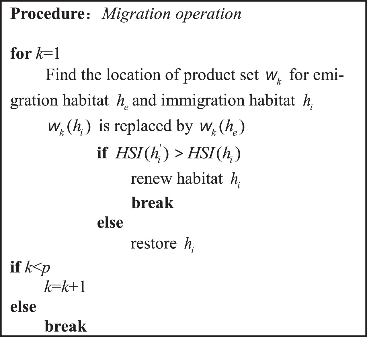
Pseudocode for migration.
The local search procedure is crucial to forcing the algorithm out of local optima. The mutation process used in this paper disrupts a specific set of jobs and associated factory allocation sets of the product, changing the chosen habitat’s appropriateness significantly. Instead of performing individual mutation procedures inside the region, the RBBO mutation operation integrates the habitats of all regions into a single region for mutation.
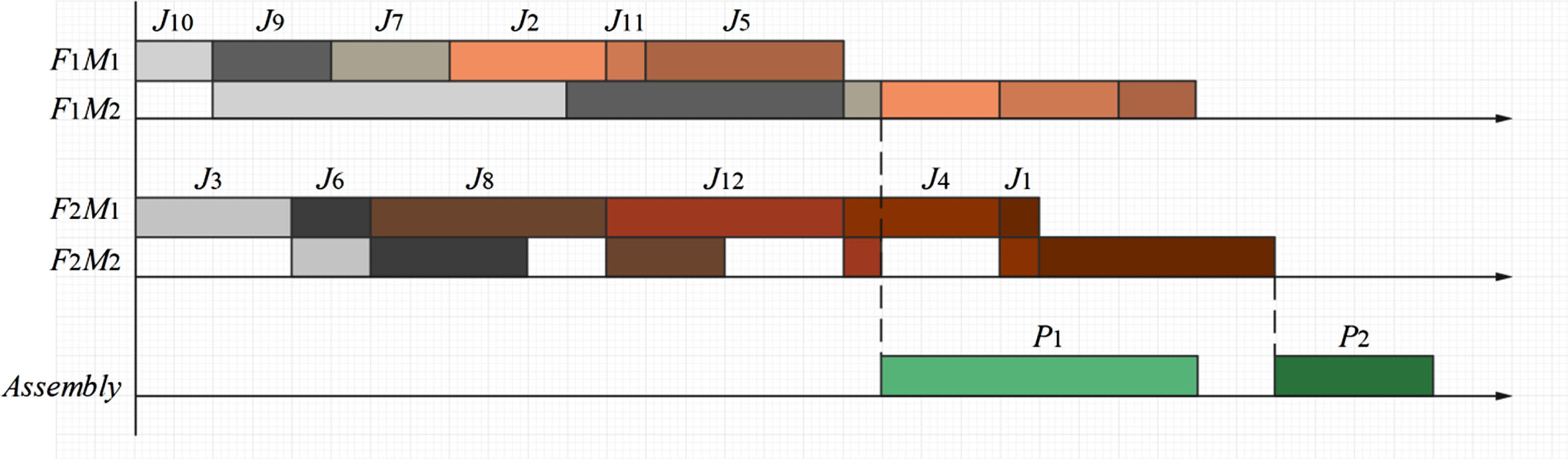
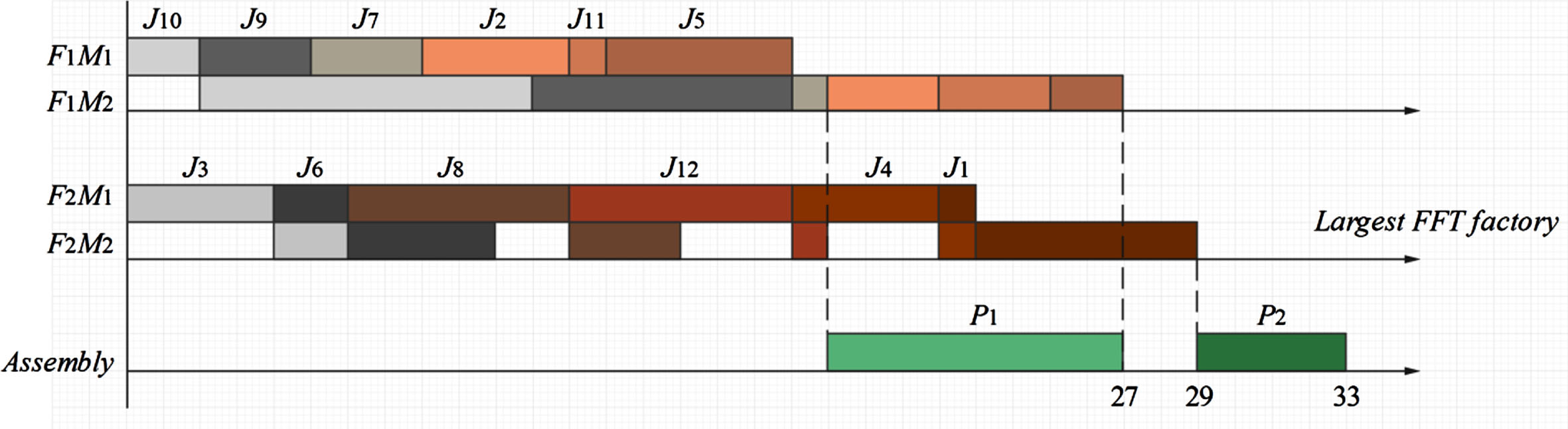
The mutation operation used in this paper is to identify critical factory optimization, lower the critical factory fuzzy finish time (FFT), and subsequently lower MFAT. Taking the example in 4.2 as an example. Assuming a mutation operation is required on the habitat h m . Find the factory with the largest FFT by decoding the h m first. Figure 5 demonstrates that factory 2 is the factory with the largest FFT. From right to left, will select products from factory 2, and that product set is ω2 = [81241]. Choose the first job from this product set, then choose a factory at random to place it in the associated product set. As the optimization target in this instance, select job 4 from product 2 in factory 2 and add it to product 2 in factory 1. In comparison to the original scheme, the sorting results based on [10 9 7 2 11 5 4] [3 6 8 12 1] are better as shown in Fig. 6. The Pseudocode for mutation operation is shown in Fig. 7.
Gantt chart of cases before mutation operations.

Gantt chart of cases after mutation operations.

Pseudocode for mutation.
The flowchart of the RBBO algorithm is shown in Fig. 8.
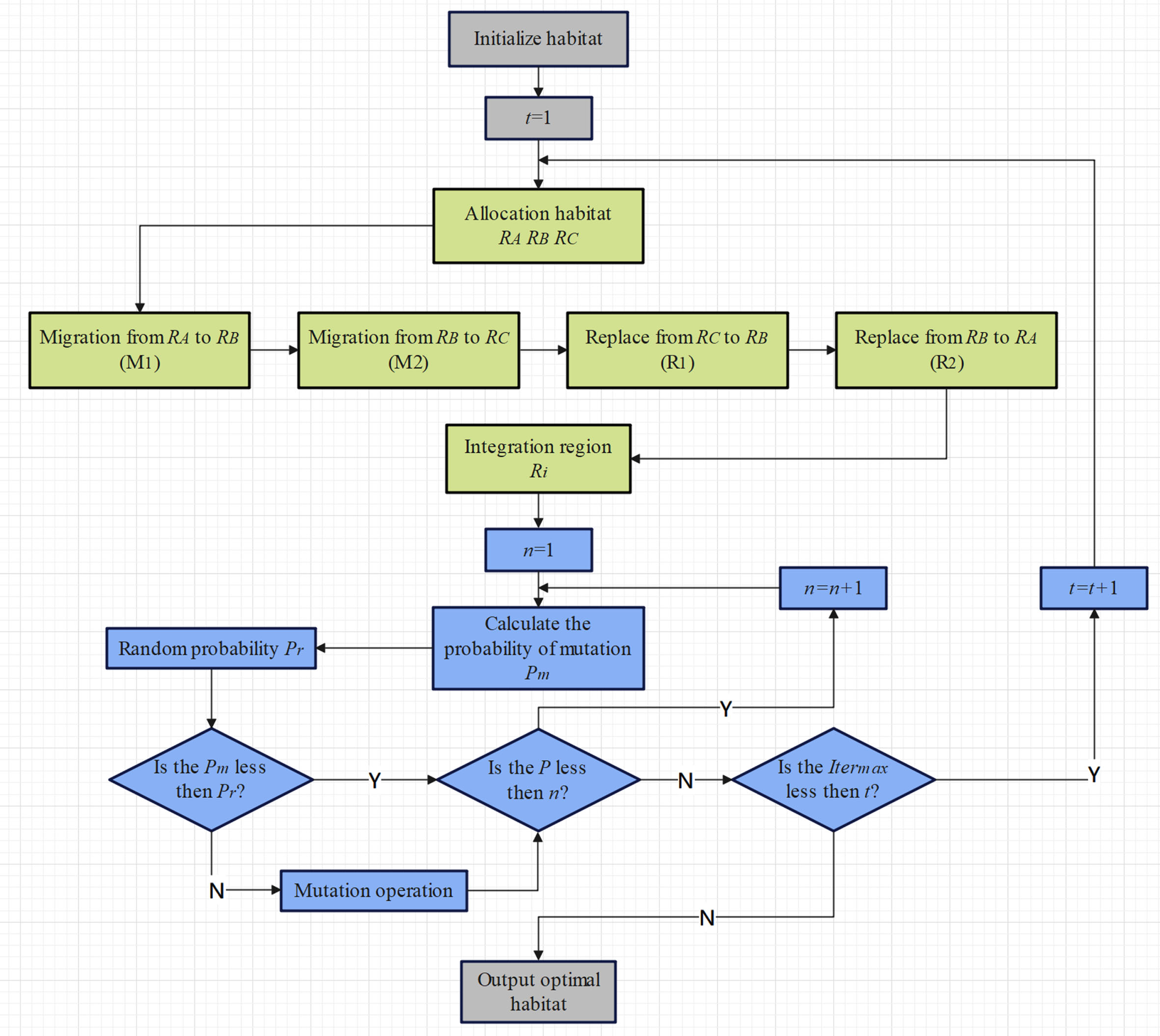
Flowchart of RBBO.
A batch of initial habitats must first be initialized, and their HSI must be determined. Based on HSI, divide the area and provide habitat to each section. It is essential to merge the habitat into one region and carry out habitat transformation activities after the migration and replacement of the current habitat region is complete. When the goal maximum number of iterations has been reached, continue the iterative process one more time, then halt the algorithm’s operation and output the HSI value of the ideal habitat.
All trials were carried out on a 16.0 RAM, 2.8 GHz CPU PC utilizing Microsoft Visual C++2022 programming. First, as shown in Table 2, created RBBO parameters and provided four sets of algorithm parameters with different accuracies. As indicated in Table 4, the orthogonal test table and average HSI (AVG) statistical results were produced using parameters with various degrees of accuracy. The Taguchi experiment was the methodology employed, with cases J = 16, M = 5, F = 4, and P = 4. Based on the information in Tables 2 and 4, the response values for each parameter in Table 5 and the response trends for each parameter in Fig. 9 were derived. Through experiments, the most acceptable parameter accuracy for RBBO can be accurately defined. The effectiveness of the algorithm must be confirmed after setting the parameters. The GA, BBO, VND, SPT, LPT, NEH and RBBO solutions that were used in the case are displayed in Tables 6 and 7. Figures 10 and 22 illustrates the algorithm’s analysis of variance, which enables us to see the algorithm’s benefits and drawbacks more easily. To verify our hypothesis about the RBBO algorithm, Figs. 11–20 shows the evolutionary trend of the FDAPFSP case under BBO and RBBO. Figure 23 compares the CPU runtime among different algorithms.
Combinations of parameter values
Combinations of parameter values
TFN corresponding ranking
Orthogonal table of parameters settings
Average response values of each parameter

The influence trend of parameters.

Analysis of variance chart between VND, GA, BBO and RBBO.

Case 1.

Case 2.

Case 3.

Case 4.
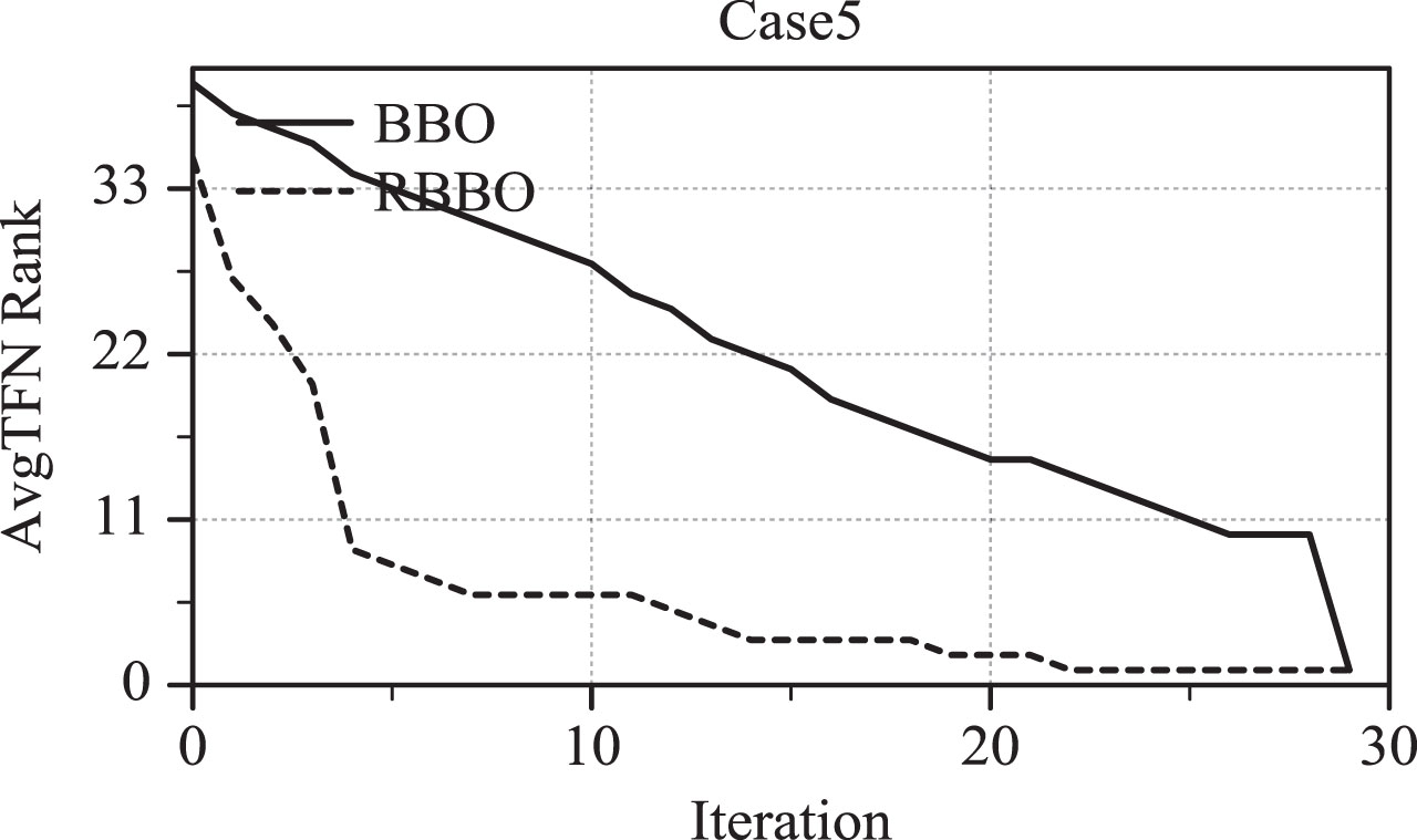
Case 5.

Case 6.

Case 7.

Case 8.

Case 9.

Case 10.

Analysis of variance chart between SPT, LPT, NEH and RBBO.

Line chart of algorithm CPU running time in FDAPFSP case.
The ten cases provided in this paper are all randomly generated based on DAPFSP basic cases through random numbers. The parameters of RBBO include the number of habitats P, the maximum mutation rate Mmax, and the maximum iteration number Itermax. This paper will use four different parameter values for the Taguchi experiments [32] with a test case. Four sets of parameter combinations will generate 16 test cases. Test each case 10 times and record the data for each test. After the test is completed, perform TFNcomparison on the data and generate a set of sorting tables from small to large. Each test TFN has its corresponding sorting sequence number, and the sorting sequence number is used to replace the TFN to generate a parameter Run chart. Calculate the average ranking (AR) of each test case. Table 4 shows the four sets of parameters provided in this paper. Table 3 shows the TFN corresponding ranking from 16 test cases. Table 4 shows the AR generated by 16 parameter combinations. Figure 6 is the parameter trend chart.
Through experiments, ten different TFNsolutions can be created. These ten solutions were ordered using the TFNcomparison approach, but rank values rather than TFNvalues were employed. These ten sets of solutions are shown in Table 5. Table 6 shows the orthogonal table of parameters settings.
It can be seen from the simulation results in Fig. 9 and the simulation results of parameter combinations in Table 7 that when P increases, the algorithm’s search performance improves and Mmax is too large or too small, it will cause poor changes in the algorithm’s performance, and so will Itermax. Therefore, choose P = 100, Mmax = 0.40 and Itermax = 30 are used to solve the problem, the RBBO algorithm has the best result. Therefore, this parameter is selected as the algorithm parameter for RBBO.
Algorithm comparison
BBO and GA were chosen for comparison testing to assess the efficacy of RBBO in FDAPFSP. Except for various algorithm models, the experiment is conducted fairly by employing the same search methodology across the board. Table 8 displays the comparison table of the outcomes. Using c2 in TFN as the comparison technique because there is presently no way that can calculate the average value of TFN. Three metrics are offered for each algorithm. The worst-case solution (WST) among the five runs of the algorithm, the best-case solution (BST), and the average output result (AVG) of the five runs of the method are all represented by the acronyms. The cases designed in this article are all based on the DAPFSP case. A total of ten cases were provided, with a size of J = {8, 12, 16, 20, 24}, M = {2, 5}, F = {2, 4}, P = {2, 4}.
RBBO’s effectiveness verification
RBBO’s effectiveness verification
The variance analysis on the test results of RBBO, BBO, GA and VND [1] in 10 separate cases allows for a more in-depth examination of the distinctions between these three algorithms. The VND termination condition is CPU runtime=F × C, where C = 0.1. GA, BBO and RBBO use the same number of iterations and population and set the termination condition to the maximum number of iterations. Figure 10 displays the Tukey’s HSD test confidence intervals at a 95% level of assurance together with the mean change curves of the three algorithms.
Table 8 and Fig. 10 show that RBBO significantly outperforms GA and VND, with RBBO’s WST, BST, and AVG values being far greater than GA’s. This shows RBBO’s advantages for handling distributed problems in an informal way. Due to its greater iteration up than BBO, RBBO provides more new solutions than BBO. It may speed up the process of mutation by quickly achieving local optima in the overall habitat. Ten sets of iterative speed images of BBO and RBBO cases were provided, and tracking and observing the overall evolution of habitats based on the optimal population of each habitat generation. In the same way, compare each TFN value using the TFN comparison method to get a Rank table. To track a trend of image changes, c2 values are used instead of TFN values.
In Table 9, by comparing the results of RBBO with six heuristic algorithms in ten FDAPFSP cases, RBBO has been found to have good local search ability and can find better solutions for each situation. meanwhile, the CPU runtime line charts of RBBO and BBO, GA, VND, and six heuristic algorithms were provided. Among them, the three heuristic algorithms SPT (short processing time), LPT (long processing time), and NEH were all taken from reference [1], and six heuristic algorithms were obtained through two different factory allocation methods in [1]. Although heuristic algorithms cannot provide the optimal solution, the quality of the solution is much better than that of the random solution, and heuristic algorithms usually have a shorter running time. Through heuristic algorithms, redundant solutions can be screened for the algorithm. As shown in Fig. 22, RBBO has an advantage in running time compared to GA and is longer than BBO, but it sacrifices some CPU running time in exchange for a better solution. This is a reasonable balancing strategy.
RBBO’s effectiveness verification
Through experiments, it was found that under these ten cases, the habitat’s development speed of RBBO was much faster than that of BBO. Due to the increase in habitat evolution speed, it is expected that the algorithm will have sufficient time to search for better solutions through local optima. This is due to the faster development speed of RBBO compared to BBO. This habitat mechanism was developed during the migration phase.
This paper proposes the problem of combining DAPFSP with fuzzy processing time constraints and designs a model for this problem. This article proposes the RBBO algorithm, designs four sets of parameters, and conducts Taguchi experiments to obtain the optimal parameter combination. Designed and solved 10 sets of examples. By comparing SPT, LPT, NEH, VND, GA, BBO, and RBBO algorithms, obtained interval graphs for the application of these three algorithms in FDAPFSP cases. To verify the hypothesis of the RBBO, iteration calculations were conducted and the iteration curves between the BBO algorithm and the RBBO were obtained.
Fuzzy processing time constraint is a common scheduling constraint in actual production and processing processes. Due to the uncertainty of processing time, it is necessary to consider reducing the difference between delayed processing time and early processing time in actual scheduling arrangements, so that this difference is close to 0. The ideal processing time value cannot be blindly regarded as the goal of fuzzy scheduling, and comprehensive consideration should be given, this scheduling arrangement is only feasible and practical.
The structural complexity of the RBBO algorithm will be reduced in future work by optimization based on the algorithm, and a new search strategy will be created to be added to it. To bring the DAPFSP problem into line with the real situation, add new constraints. To determine which method is most self-adaptive, an attempt will also be made to combine the new algorithm with the BBO. As an instance, consider the krill swarm algorithm [34, 35] and the grey wolf optimization method [33].
Footnotes
Acknowledgments
This work was supported by Anhui Provincial University Research Projects(2023AH050935), the Research Initiation Foundation of Anhui Polytechnic University (2022YQQ002), Anhui Polytechnic University Research Project (Xjky2022002), the Open Research Fund of Anhui Key Laboratory of Detection Technology and Energy Saving Devices (JCKJ2021A06, JCKJ2022B01), Key Natural Science Research Projects of Colleges and Universities in Anhui Province (2022AH050978, 2023AH052915), Anhui Province University Excellent Top Talent Training Project(gxbjZD2022023), Wuhu science and technology project (2022jc26), and Anhui Polytechnic University-Jiujiang District Industrial Collaborative Innovation Special Fund Project (2022cyxtb6).