Importance of data preprocessing in time series prediction using SARIMA: A case study

Abstract

Over last decades, time series data analysis has been in practice of specific importance. Different domains such as financial data analysis, analyzing biological data and speech recognition inherently deal with time dependent signals. Monitoring the past behavior of signals is a key for precise predicting the behavior of a system in near future. In scenarios such as financial data prediction, the predominant signal has a periodic behavior (starting from beginning of the month, week, etc.) and a general trend and seasonal behavior can also be assumed. Autoregressive Integrated Moving Average (ARIMA) model and its seasonal extension, SARIMA, have been widely used in forecasting time-series data, and are also capable of dealing with the seasonal behavior/trend in the data. Although the behavior of data may be autoregressive and trends and seasonality can be detected and handled by SARIMA, the data is not always exactly compatible with SARIMA (or more generally ARIMA) assumptions. In addition, the existence of missing data is not pre-assumed in SARIMA, while in real-world, there can be always missing data for different reasons such as holidays for which no data may be recorded. For different week days, different working hours may be a cause of observing irregular patterns compared to what is expected by SARIMA assumptions. In this paper, we investigate the effectiveness of applying SARIMA on such real-world data, and demonstrate preprocessing methods that can be applied in order to make the data more suitable to be modeled by SARIMA model. The data in the existing research is derived from transactions of a mutual fund investment company, which contains missing values (single point and intervals) and also irregularities as a result of the number of working hours per week days being different from each other which makes the data inconsistent leading to poor result without preprocessing. In addition, the number of data points was not adequate at the time of analysis in order to fit a SARIM model. Preprocessing steps such as filling missing values and tricks to make data consistent has been proposed to deal with existing problems. Results show that prediction performance of SARIMA on this set of real-world data is significantly improved by applying several preprocessing steps introduced in order to deal with mentioned circumstances. The proposed preprocessing steps can be used in other real-world time-series data analysis.

Keywords

Time series data prediction SARIMA data preprocessing

1. Introduction

Analysis of time series data is an active area of research in data science [13, 19]. Different mathematical models have been proposed for time series forecasting. Time series data are often challenging to work with, due to their inherent complexity. Autoregressive Integrated Moving Average (ARIMA) model is one of the widely used models for linear time series prediction, which is known to have significant accuracy and is flexible in representing different types of time series. ARIMA has been successfully applied in order to analyze real-world time-series data [12, 2, 29, 16, 30, 3] particularly financial data [24, 7, 27], and is also extended for online time series forecasting, in which the data has a streaming nature [25].

ARIMA model is composed of an autoregressive and a moving average part, each specified by a parameter. Detail definitions of ARIMA and its seasonal extension, SARIMA, is provided in Section 2. In ARIMA $(p,d,q)$ , parameter $p$ defines the order of autoregressive part, and $q$ defines the order of moving average part. $p$ specifies the number of previous observations used to predict future values and $q$ specifies the number of error terms that should be integrated into the moving part of the model. Parameter $d$ specifies the order of differencing. Differencing is a technique used to make the series stationary. A value of one for $d$ for example, means the first order difference of values $(y_{t}-y_{t-1})$ is used instead of original observations. Orders $p$ and $q$ can be determined using autocorrelation analysis. Definition of ARIMA model is based on assuming regularities in data based on which $p$ , $q$ and $d$ can be fitted.

This mathematical model is designated for analyzing linear form time series, however there have been different studies that still make use of its benefits when the data is a composition of linear and non-linear signals [34]. Most of real-world data consists of both linear and non-linear correlation structure among data values, therefore a linear model such as ARIMA would not be capable of modeling the mixed pattern underlying such data. Artificial Neural Networks (ANNs) on the other hand is a machine-learning based method for analyzing non-linear time series and has not shown notable accuracy in modeling linear time series data. For this reason, different models have been proposed in order to first decompose the signal into linear and non-linear parts, and then analyze each component using the proper model. It has been shown that a combination of linear and nonlinear methods is a better choice for modeling real world data compared to an individual linear or nonlinear model [6]. There is notable literature on applicability of ARIMA beside non-linear models such as ANNs for precise time series forecasting, which demonstrates the proficiency of ARIMA model in real-world data even when the data contains non-linear signals [34, 22, 16, 10, 23, 28]. One example is [20], in which the time-series observed data is considered to be the sum of a linear and a non-linear component. Based on such assumption, the authors proposed a hybrid model based on ARIMA and deep belief networks (DBN) in order to forecast time-series data; in this method ARIMA is applied to predict short-term data and DBN is then used to predict the error of the ARIMA model. The error is the difference between the real data values and the predicted ARIMA-based values, which is considered to be the nonlinear component of the data, and is modeled using a DBN. The final prediction is then calculated based on ARIMA prediction plus predicted error from DBN part. In [21], Discrete Wavelet Transform (DWT) has been used in order to improve the precision time series prediction, by decomposing the time series into linear and non-linear parts, and using ARIMA and Neural Network for predicting the corresponding linear and non-linear parts respectively. With improvement in computational power using GPUs, more sophisticated machine learning algorithms are used to analyze non-linear methods. Long short-term memory (LSTM) deep network is one of popular tools for analyzing non-linear time-series data, and has been shown to outperform ARIMA in non-linear data analysis [16].

ARIMA model is extended to capture seasonality of the data, resulting in Seasonal ARIMA model formulated as $\text{SARIMA}(p,d,q)\times(P,D,Q)^{S}$ . By seasonal behavior we mean a pattern that is repeated every season, every month, every week, etc. per year. A seasonal behavior makes the data dependent on seasonal lags. For example, for monthly data similar components are observed in similar months from previous years (multiples of $s=$ 12). In order to build a more precise seasonal model, we need the data to be exactly fit to this pattern and again missing values for one lag can be source of errors in the model fitting.

To summarize, a data value in SARIMA is predicted as a function of past data values. SARIMA is composed of a non-seasonal and a seasonal component. Each component has its own parameters regarding to autoregressive and moving average behavior of the model determining which previous data (autoregressive part) or error values (moving average part) should be considered to predict a desired data value. Differencing is hired in order to make the series stationary. Figure 1 represents a summary of SARIMA parameter details. Details on SARIMA are provided in Section 2 (Eqs (1)–(2)).

Figure 1.

An overview of SARIMA model parameters.

SARIMA, is also widely used for analyzing financial data [17, 1, 14, 31]. ARIMA is capable of capturing autoregressive and moving average behavior of the data, while financial data usually follow a seasonal pattern. SARIMA model is also used in combination with other models such as support vector regression [33] and long short term memory (LSTM) networks [35] in order to provide a better prediction.

Preprocessing is an important step in data analysis tasks for cleaning real data which is noisy, missing and inconsistent. Data preprocessing improves the quality of data and hence the models generated from it [18]. In the current work we focus on presumptions of ARIMA and its seasonal extension, and how data preprocessing can come in handy when fitting SARIMA models on real world data.

When the time-series data is not preprocessed and clean (for example in existence of missing data), this regularity in the time-series is not further preserved, and therefore the model will be misled in the parameter fitting process (since a number of data values for which $p$ , $q$ and $d$ are set are not available in the data or include inconsistencies). By missing data, we mean the data records which are not present because of reasons such as holidays.

The goal of this work is to investigate how in a real scenario the mentioned properties of the data can mislead the SARIMA model, and how preprocessing can overcome this problem. In the rest of this paper, we first introduce ARIMA and SARIMA models (Section 2) and then investigate how several preprocessing steps can improve the quality of SARIMA (Section 3). Experimental result and discussion parts are provided in Sections 4 and 5 respectively.

2. ARIMA and SARIMA models

Autoregressive Integrated Moving Average (ARIMA) model is one of the most frequently used models for analyzing time series data. ARIMA is a stochastic model which can be applied on the data given specific assumptions such as linearity of the data and also the data should be following a specific statistical distribution. ARIMA model is defined based on an auto regressive (AR) part [27, 20], an integrated (I) part and a moving average (MA) part. The AR concept assumes the data is regressed on its own lagged values. Seasonal ARIMA (SARIMA) is a variation of ARIMA for seasonal time series data analysis.

Autoregressive models predict a data value using its past observations. Considering AR $(p)$ , an autoregressive model of order $p$ , a prediction on $y_{t}$ is formulated as follows:

$\displaystyle y_{t}=\sum_{i=1}^{p}w_{i}y_{t-i}+b+\varepsilon_{t}$ (1)

in which $b$ is a constant (bias) term, $\varepsilon_{t}$ is a random error at time $t$ , and $w_{i}$ s are regression model parameters. A moving average model of order $q$ , MA $(q)$ , uses past errors as its explanatory variables. These error terms are considered to be independent and identically distributed (generally normal distribution assumption with mean zero). The MA $(q)$ can be written as:

$\displaystyle y_{t}=\mu+\sum_{i=1}^{q}\theta_{j}\varepsilon_{t-j}+\varepsilon_% {t}$ (2)

Autoregressive moving average (ARMA) models are formed by combining AR and MA models and are represented as:

$\displaystyle y_{t}=b+\varepsilon_{t}+\sum_{i=1}^{p}w_{i}y_{t-i}+\sum_{i=1}^{q% }\theta_{j}\varepsilon_{t-j}$ (3)

In an ARMA $(p,q)$ model, parameters $p$ and $q$ refer to the parameters of autoregressive and moving average parts respectively. Considering lag function $L$ defined as $L^{i}y_{t}=y_{t-i}$ , it can be easily observed that ARMA model can be re-written as:

$\displaystyle\left(1-\sum_{i=1}^{p}w_{i}L^{i}\right)y_{t}=\left(1+\sum_{j=1}^{% q}\theta_{j}L^{j}\right)\varepsilon_{t}$ (4)

It is worth to mention that assumption of time series data being stationary is usually considered in order to simplify developing mathematical models, such as ARMA, for statistical processes. Since time series data may demonstrate seasonal or trend patterns in real data cases, this assumption will be violated; hence techniques such as differencing and power transformations are used in order to remove these patterns.

ARIMA is an extension of ARMA model which can be applied on non-stationary data as well. ARIMA uses a technique called differencing is used to make the data stationary by removing trends. In differencing, the d’th order differences of data is considered to build the ARMA model. The mathematical formulation of Autoregressive Integrated Moving Average (ARIMA) using lag function can be written as:

$\displaystyle\left(1-\sum_{i=1}^{p}w_{i}L^{i}\right)(1-L)^{d}y_{t}=\left(1+% \sum_{j=1}^{q}\theta_{j}L^{j}\right)\varepsilon_{t}$

in which $(1-L)$ is the backward differencing operator, and $d$ specifies the order of differencing. In ARIMA $(p,d,q)$ , $p$ and $q$ are the orders of autoregressive and moving average, and $d$ is the order of integrated part of the model. $d$ is the level of differencing. If $d=0$ , the model would be equivalent the ARMA model. ARIMA model is suitable for non-stationary non-seasonal observations. Box and Jenkins. [8] have proposed a seasonal version of ARIMA (SARIMA), in which seasonal differencing is used to remove seasonal non-stationarity. For example, $z_{t}=y_{t}-y_{t-S}$ is a first order seasonal difference of data $y$ , in which $S$ determines the season period in which the data can be repeated; $S=$ 12 for example specifies a monthly time series in which data of a month is proportional to the data in the same month previous year. SARIMA is usually represented as SARIMA $(p,d,q)\times(P,D,Q)^{S}$ , and is formulated as follows:

$\displaystyle\left(1-\sum_{i=1}^{P}w_{i}L^{S^{i}}\right)\left(1-\sum_{i=1}^{p}% w_{i}L^{i}\right)$ $\displaystyle(1-L)^{d}(1-L^{S})^{D}y_{t}$ $\displaystyle=\left(1+\sum_{j=1}^{Q}\theta_{j}L^{S}\right)\left(1+\sum_{j=1}^{% q}\theta_{j}L^{j}\right)\varepsilon_{t}$ (6)

As mentioned about ARIMA earlier in this section, lag function $L$ defined as $L^{i}y_{t}=y_{t-i}$ determines which previous time points should be considered in order to predict $y_{t}$ . As an example the term $(1-\sum_{i=1}^{P}w_{i}L^{S^{i}})$ represents which previous values of $y$ (i.e. $y_{t-1},y_{t-2},\ldots,y_{t-i}$ ) should be used in the autoregressive term of the seasonal part of the formula. Model parameters can be estimated using tools such as complete and partial autocorrelation functions. Grid search method can also be used for fitting the parameters of SARIMA.

3. Data preprocessing for seasonal ARIMA

Data analysis methods, often presume some criteria on the data. Assumptions such as specific statistical distribution, completeness of data, and consistency. That’s while real world data is highly susceptible to missing, noisy and inconsistent values. In order to build reliable models, one necessary step is taking care of model assumptions not being violated and the input data being correctly preprocessed. General preprocessing steps such as removing noise and inconsistencies in the data and handling missing values (data cleaning), decreasing data size by removing redundant features or methods such as clustering (data reduction), normalization and transformation of the data into acceptable range (data transformation) are introduced in a standard data mining process in order to guarantee data quality, however each statistical or machine learning based model usually have specific assumptions considering which will lead us to a limited set of preprocessing tasks which can be applied on the input data. In this section, first the data is introduced. Then considering details of ARIMA model definition, application of a set of necessary data preprocessing steps before applying ARIMA are discussed on a case study of financial data. In Section 4, the result of applying preprocessing steps on the data is presented.

3.1 Data description

Our data is derived from transactions of a mutual fund investment company. The data in this company, is recorded on a daily bases, but the goal of the company is to predict the monthly sum of investments. At the time of analysis, the data was only available for nine months which was not sufficient for monthly-based SARIMA prediction. The data consists missing values; for holidays there are no data available. Also, for the last day of each week, the working hours is almost two third of the working hours in the rest of the days. In order to analyze this data, several preprocessing steps has been performed. In the following subsections we discuss each preprocessing step and why they are necessary with respect to the nature of the data and also assumptions of ARIMA model. In Section 4, the results regarding to effectiveness of this preprocessing steps are presented.

Figure 2.

A sample of case study series data available in (a) daily based resolution, and (b) monthly based resolution.

3.2 Data resolution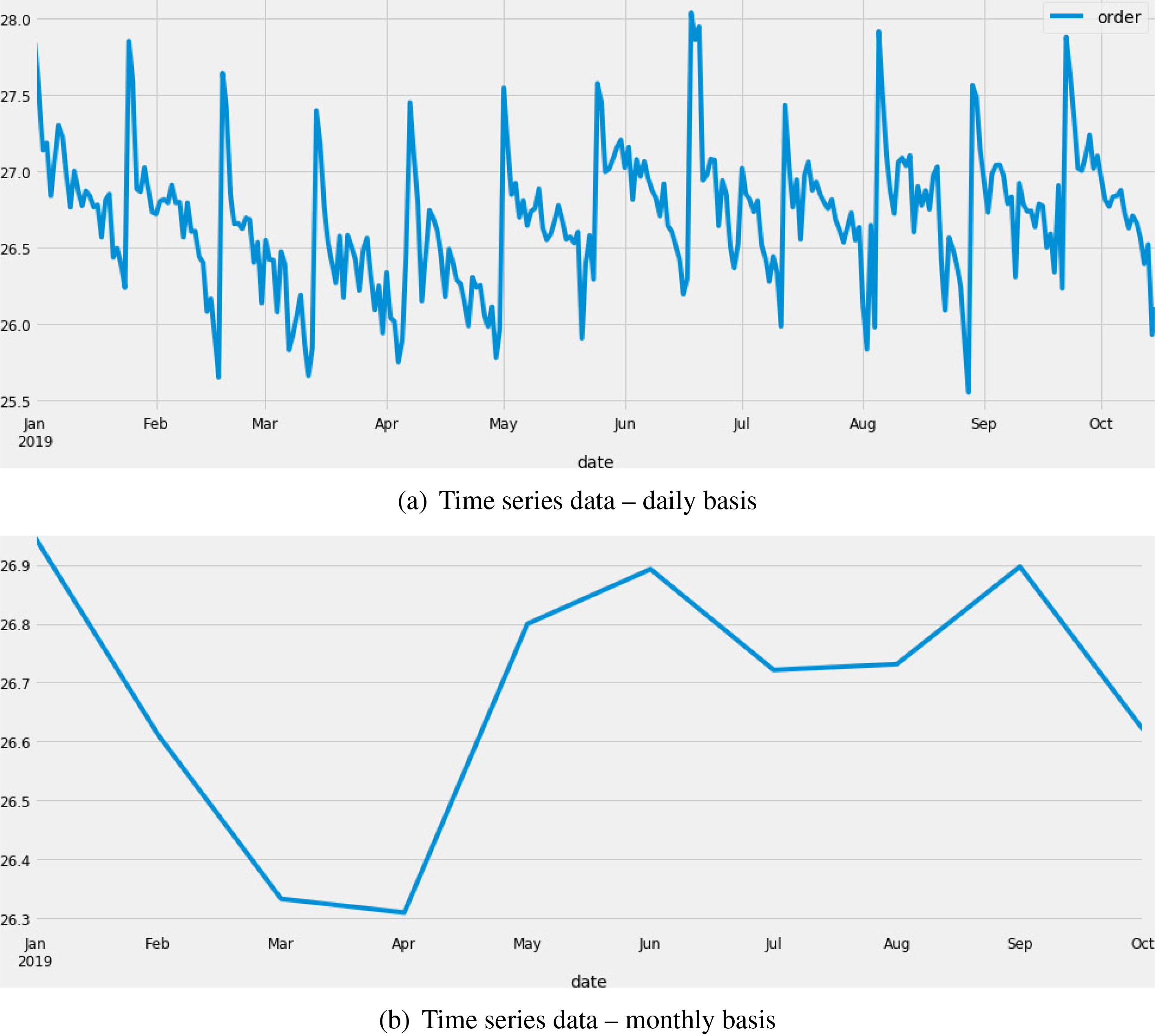

Selecting proper level of data resolution plays an important role in time series analysis. A daily-based pattern might not be visible anymore when the resolution is weekly-based. The choice of data granularity can also naturally be made with regard to the granularity of the predicted values. For example, if the goal is to predict the monthly value of income, then the monthly-based data can be used for constructing the model.

In the case under study, the goal was predicting the sum of the investments for the upcoming months. Natural resolution to select for this data is monthly data. The first problem aroused here was that our data in month level was not in enough quantity for fitting the SARIMA model, since the seasonality behavior will be not visible in this level. The other problem was having insufficient data points for fitting non-seasonal ARIMA. For monthly data, we may expect a seasonality of 12, i.e. data for each month is proportional to the data of the same month in previous year. In situations like this, we need at least monthly data of two consecutive years in order to capture the seasonality pattern, which was not available at the time of analysis. One solution to this problem is to delay the data analysis process until the date is complete, which is not desired since this strategy would delay the benefits of prediction for about one year.

Figure 3.

Investment value over a 9-month period (a) Missing data values in the dataset; (b) missing values filled with zero can mislead the model fitting process.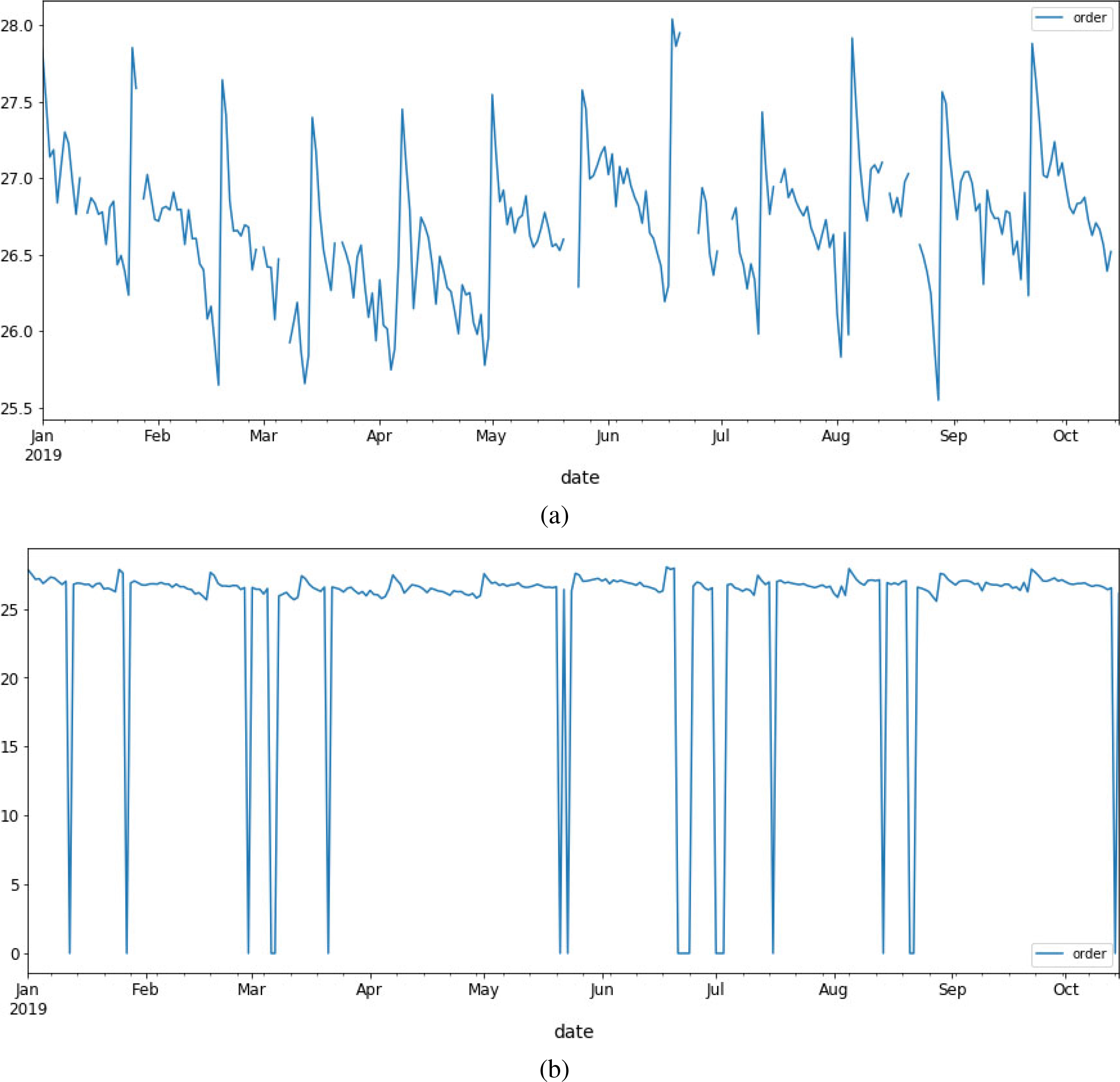

Our solution in this case, was to use data on a daily basis, because there exists sufficient data at this resolution and also final values for each month can be calculated using the daily predicted values of the corresponding month. Using daily values, we may lose the seasonal patterns, but due to the limitation in the number of data values this remains as the only one solution. As the result, in order to predict the company’s investment amount for a month, first the daily data for that month is predicted and the target value for the target month is then estimated by integrating over the predicted values for days of the corresponding month. Existing holidays in the data used to build the model and also in the month to be predicted will have an effect on the output, which is handled by a preprocessing and postprocessing step explained in Section 4.1. Using these pre and postprocessing steps, the integration of daily data is applied after handling holidays in the data used for fitting the model and also the predicted data. If we explore the data on a daily resolution, patterns repeated in periods less than one month (such as weekly patterns) may be observed. Figure 2 demonstrates the data at these two different resolution levels. Although the prediction is desired at month level, the data at this level is no sufficient and even no seasonal pattern is observed at month level in our dataset (Fig. 2b). In day-level data, month level seasonal patterns may be missed (and instead daily seasonal patterns be fitted), but the data is sufficient to make reasonable predictions for a whole month.

3.3 Handling missing data

SARIMA model is not capable of handling missing values inherently, and the model is developed assuming that the data is complete. Therefore, before applying SARIMA on any dataset, handling missing data should be considered as a preprocessing step. Different approaches for handling missing data have been introduced in data mining literature [18]. A review of these approaches will be summarized here and then our approach, which is customized to SARIMA model assumptions, is introduced. Ignoring the tuples with missing value is an approach which may be useful in some context (especially when the number of records containing missing values are not noticeable). Other naïve approaches are filling the missing values with a global constant such as ‘unknown’ or a presumed number, filling the missing values manually, use mean or median value, and filling the missing values with the most probable values. It’s intuitive to see that filling missing values by constants or even mean or median values may mislead ARIMA model inference. ARIMA is an autoregressive model and the regressor weights can be affected by the approach taken in order to fill missing values. The filled missing values may also mislead the differencing part of the model which is necessary for making the time series stationary.

In existing published research, ARIMA is usually applied on data without missing value, however the existence of missing value is a natural assumption for the data. Several approaches have been proposed in the literature for filling missing values before applying ARIMA [4, 15, 32, 5].

There are two types of missing values in the dataset under study. One is single-day missing values (or single day holidays), and one is longer holidays (such as new year) which will dramatically reduce the number of data points which SARIMA expect to have for one month. Figure 3a represents the missing intervals in the dataset. Removing missing data records will affect the parameter fitting of SARIMA, since orders $p$ , $q$ and $d$ of model specifies the number of past data or error values to be considered for prediction. On the other hand, filling these values with zero will obviously mislead the model (Fig. 3b). Our approach here was to fix the number of the days per month to a value (we used 24, which is the number of working days per a typical month without holidays). By this approach, first we maintain the period of original patterns observed in the data which makes the data matched to SARIMA assumptions and second, we don’t dramatically change the data by inserting zeros. The process for handling missing values is designed to fill single-point missing values using linear interpolation and for missing value intervals, such as new year holidays, the interval is predicted using SARIMA model fitted on previous months data plus the available data from current month in case the missing interval does not occur at the beginning of the month. More detail on this approach is provided in Section 4.2.

Having the number of days fixed per month is a rational choice since by this technique SARIMA model will be able to successfully fit the differencing, autoregressive and moving average part of the model. To better understand this point, consider a seasonal data with monthly seasonality, autoregressive term of order 5, and differencing of order 2. In this data, we expect to have 12 values per year. In case the number of data points are not fixed per year, the prediction of points which should depend on values from one year ahead and also depend on a specific differencing order, will be estimated using the wrong data points.

In our study, we inferred single-point missing values inside a month interval using linear interpolation. In case there are several missing values, we use ARIMA model trained on previous months and available data from current month in order to predict the missing interval.

3.4 Data consistency

One of the preprocessing steps that was applied on the data was making the data values regarding the last working day of the week consistent to other values (we had six working days per week). For the last (sixth) working day of each week, the working hours at the company was two third of working hours of other days. We considered this fact as the source of higher values of error for the last working day of each week. To make the data consistent in this sense, the mentioned data values were multiplied by 3/2. Finally, after the model is fit and the output is predicted, the values of mentioned days are again transformed to their original values in a postprocessing step by multiplying by 2/3.

3.5 Data transformation

Removing seasonality and trends is one important data transformation step in time series data analysis. Weather data contains these patterns can be detected by visualization techniques. Plots can also reveal if there is any sharp change in the behavior of data, or if there’s any outlying behavior [9]. Different techniques may be applied on the data in order to remove seasonality, including those which estimate the components to be removed and subtract them from the data, and those who depend on differencing. Differencing (details are provided in Section 2) is a common method in removing trends and seasonality. Using this technique, a differencing order d (a positive integer) is specified, and data points $X_{t}$ are replace with ( $X^{\prime}_{t}=X_{t}-X_{t-d}$ ). Regardless of the technique, the result is a stationary time series, whos values are refered to as residuals.

Logarithm transformation can also be applied on the data if the fluctuations are seemingly to grow linearly (applying logarithm transformation makes fluctuations closer to constant magnitude). While logarithm transformation is considered as a presumed preprocessing step in some research, it is important to note that if the data has an additive behavior, which is also assumed by SARIMA, there’s no need for this transformation step. If the goal is to capture a multiplicative seasonal pattern, logging the data prior to model fitting can be beneficial. While inferring differencing parameter $d$ is a standard process in ARIMA, log-transformation has not been observed to be always useful. The effect of log-transformation in our specific case will be discussed in Section 4.4.

4. Results

Four experiments have been conducted on the data to test the effect of preprocessing steps introduced in sections 3.2–3.5. Our code is implemented in Python 3.7, and ARIMA-related functions are imported and used from package statsmodels.

4.1 Choosing correct data resolution

As explained in Section 3.2, our goal was to predict monthly sum of investments. At the end of analysis period only sixteen monthly data points were available. In the beginning, the data for 9 months was available which we used to predict the 10 ${}^{\text{th}}$ month. Gradually the data was completed until the end of analysis in which the data of a sixteen-month period was available. The major challenge was that the data was not enough to build our SARIMA model for monthly based data. As the result, we decided to use daily-based data. For predicting the total sum of investments for each month, first we fitted a model to predict daily investment values of the regarding month and then the sum of daily-based data per month was used for monthly based predictions. In this process however, there were several important issues such as the number of working days per month was not equal for every month (due to existence of holidays). In addition to violating SARIMA model assumption of having fixed number of lag values available for each prediction, this could affect the total sum of investment for a given month, and therefore changes the predictions for the incoming months. To solve this problem, we fixed the number of days per month to 24 working days. Holidays missing values were filled out through a process explained further in Section 4.2.

After predicting the daily-based values for a given month, we applied a postprocessing step to replace the data values for holidays with zero. Therefore, we don’t have an overestimation of monthly sum of data. The error finally is calculated on the postprocessed values. Here the results for the last five months are reported. For all of the predictions in our experiments an interval of the past 12 months data is used in order to fit the model. Table 1 represents the result of the final model (after applying all preprocessing and postprocessing steps). The relative error which was acceptable for this case study is reported.

Table 1
Real vs. predicted monthly investment values. The prediction is done based on the past 12 months. This final model is achieved after examining the proposed preprocessing steps described in Sections 3.2–3.5

Month	Relative error
Month 1	8.016310478
Month 2	11.31571192
Month 3	14.75353045
Month 4	10.09726242
Month 5	2.933988992

4.2 Handling missing data

As we have discussed so far, missing data can lead to two problems. Different number of working days per different months violate the ARIMA assumptions, since the autoregressive, seasonal or cyclic pattern underlying the data cannot be perfectly learned by an ARIMA-based model in case of having irregular records of data. To overcome this problem, we assumed each month to have a fixed number of 24 working days. Single-day holidays are filled out using simple linear interpolation technique. If a month contain a period of missing values (new year holidays for example), we first use the SARIMA model in order to predict the values for the missing intervals. For predicting each month’s data, the values of the past 12 months (each including 24 working days) is used.

Figure 4 demonstrates the data values and the one-step ahead predicted values for a 9-month interval. As it can be observed in Fig. 4a, there are single point and interval missing values (shown with zero in the corresponding plot). These missing values are filled in the final analysis; the result is presented in Fig. 4b. Having these daily missing values filled, improves the monthly-based prediction because our final prediction value for each month is computed by integrating daily-based data. In addition, the model parameters and regressor coefficients are better fit when the data values are not filled with non-informative zeros instead of a real estimation of investment amounts.

Figure 4.

real versus predicted data values, (a) without and (b) with filling missing values.

Table 2 represents the result of applying the model without handling missing data. As it can be observed from the table, a significant reduction in relative error is achieved after applying this preprocessing step. For all of the predictions an interval of the past 12 months data is used in order to fit the model.

Table 2

Relative error of monthly investment predictions. The prediction is done without filling missing values. The %improvement column shows the improvement of prediction after applying the proposed method for handling missing values for which except for one case, the relative error is significantly decreased by applying the proposed method for filling missing value

Month	Relative error no preprocessing	Relative error with preprocessing	%Improvement with preprocessing
Month 1	3.622374375	8.016310478	$-$ 4.393936103
Month 2	30.61377997	11.31571192	19.29806805
Month 3	33.77375685	14.38022490	19.39353195
Month 4	19.66872999	10.09726242	9.571467572
Month 5	18.35465187	2.933988992	15.42066287

4.3 Ensuring data consistency

In our case study the number of working hours varies between week days. However, ARIMA based models perform prediction based on a set of parameters fitted on the data regardless of whether there are exceptional rules for specific data points. In our case, the number of working hours, during which the investment option is open in the company and new data can be added to the daily data, only the same for first 5 working days of the week. On the sixth day, the number of working days is decreased to two third. In order to deal with this inconsistency, we used a coefficient $\alpha_{\text{adjust}}$ to be multiplied to the data values for the 6 ${}^{\text{th}}$ day in the preprocessing step in order to compensate for the decrement of working hours. In the postprocessing however, we have to return back the data to its expected value proportional to the true number of working hours by multiplying the predicted value by $\frac{1}{\alpha_{\text{adjust}}}$ to make it comparable with the real values. Table 3 shows our experiment results without applying the adjustment coefficient.

Table 3
Relative error of monthly investment predictions. The prediction is done without applying the proposed method for handling inconsistency related to the number of working hours. The %improvement shows the improvement of the final model with considering the proposed methods for handling inconsistent data. Negative %improvement shows that applying this preprocessing step, has resulted in a worst prediction (higher prediction error) compared to its non-using

Month	Relative error – preprocessing	Relative error – no preprocessing	%Improvement with preprocessing
Month 1	6.923961919	8.016310478	$-$ 1.092348559
Month 2	13.243814390	11.31571192	1.928102473
Month 3	5.590155432	14.38022490	$-$ 8.790069468
Month 4	8.961263432	10.09726242	$-$ 1.135998988
Month 5	13.327452380	2.933988992	10.393463380

Prediction using this preprocessing step however has a dramatic negative effect on prediction of month 3. As far as we investigated the data, when the last working day of a week happens to be at the start of the month, and there exists holidays in the previous month, the number of investments increases and naturally even during fewer working hours in order to compensate for the lack of number of former working days. So here we are not dealing with a straight-forward rule. Developing a technique for considering external signals is suggested to improve this model.

4.4 Effect of data transformation

Data transformation is considered as one of important preprocessing steps in data analysis. Log transformation is used in order to stabilize the variance of data and make the data look more like normal distribution, however, existing literature shows this is not always the case [26, 11]. In the existing data, log transformation does not show any improvement on the model (Table 4), and in many cases even results in an increase in the prediction error (negative values in %improvement column).

Table 4
Relative error of monthly investment predictions. The prediction is done after applying log transformation to the data. Compared to the result of the methods when log transformation is not applied, the relative error has been increased (so a negative %improvement is reported as the effect of data transformation)

Month	Relative error with log transformation	Relative error without log transformation	%Improvement with preprocessing
Month 1	8.35	8.016310478	$-$ 0.333689522
Month 2	28.35	11.31571192	$-$ 17.03428808
Month 3	12.74	14.38022490	1.64022490
Month 4	13.37	10.09726242	$-$ 3.27273758
Month 5	20.65	2.933988992	$-$ 17.71601101

5. Discussion

In the current study, we investigated the usefulness of applying specific preprocessing techniques along with SARIMA model for time series data prediction. The case study data is real data derived from transactions of a mutual fund investment company. The goal of company at the time was to predict the monthly sum of investment for the next month. The data was available in days. The first challenge in the model fitting process was insufficiency of available monthly-based data for fitting a seasonal ARIMA model. One intuitive solution in such situation is to postpone the data analysis process until the time enough data is collected. But obviously companies don’t want to lose their time and benefit of the data analysis. In order to deal with this problem, we came to the idea of using daily based data and predict daily based data for the next month, hoping that we can get a good enough prediction in day-level so that we can use their summation for the monthly prediction. The daily based data however, was not straightforward to work with.

Considering the daily based data, one issue was that there existed several missing data in each month. Missing data may regard to single day holidays, or longer holidays (like new year’s holidays). In order to fit an ARIMA based model to the data, we need to have months data of equal number of days, therefore a method for filling missing data is proposed in this study; linear interpolation for single-day missing values and using ARIMA-based prediction using the data of previous month for longer missing intervals. In addition, an inconsistency is observed in the data; the number of working hours is not the same for all working days (it’s less for the last working day of the week). The lower number of working hours per day, affects (decreases) the investment amounts inherently. We tried to address this issue in the current study: applying a coefficient in order to manually increase the investment values for days with lower working hours. Experiments showed this technique is not promising and it increases the relative error in some cases. By exploring the data, we came to this conclusion that there are other factors influencing the investment values, such as if the mentioned day is in the beginning of the month or in addition if there exist holidays in the last days of previous month, the lower amount of investments will not be observed. Other methods can be considered in order to model external factors and can be tested on the data. ARIMA-based models are just autoregressive models which cannot cover these cases. Finally, we applied log-transformation on our dataset. Our experiments show that applying log-transformation is not proper in this case study and even leads to a significant increase in relative error. To summarize, this study demonstrates the importance of applying proper preprocessing techniques for ARIMA-based model fitting. In addition to common advantages such as handling missing values, data preprocessing is beneficial in making the data configuration a better match to what input format is expected by the model.

6. Conclusions

In the current research, we investigated the applicability of SARIMA model on predicting real world time series data of a mutual fund company. Since ARIMA based models, such as SARIMA, assume the data is complete, existence of missing values misleads the model fitting process. Applying preprocessing steps such as filling missing values, data transformation and selection of data resolution are preprocessing techniques which are widely used in data mining context. In this work we explored the benefits of application of these preprocessing steps before fitting a SARIMA model. Our experiments demonstrated that if these preprocessing steps are customized to best fit the data to SARIMA assumptions, the prediction accuracy of the final model will be increased significantly. Also, we showed that when the data at its natural granularity for prediction is not adequate, data at a greater level of granularity can be used. As an example, in this work we used daily based data for month level predictions. We showed that this change in granularity involves certain issues which can be addressed properly using pre and postprocessing techniques. Finally, we provided examples of data inconsistency sources in our case study, resulted from the effect of external sources. In our case, there were unusual observations at the start or end of a month. We tried to moderate the effect of this external source using preprocessing. Integrating these inconsistencies as an external signal into SARIMA model can be considered for future work.

Footnotes

Acknowledgments

Zahra Narimani and Amir Hossein Adineh would like to thank Institute for Advanced Studies in Basic Sciences (IASBS) for providing the facilities for doing this project.

References

Al-Gounmeein

R.S.

and Ismail

M.T.

, Forecasting the exchange rate of the jordanian dinar versus the US dollar using a box-jenkins seasonal ARIMA model, Computer Science 15(1) (2020), 27–40.

Alaskar

et al., Nanoparticle and microparticle flow in porous and fractured media – An experimental study, SPE Journal 17(4) (2012), 1160–1171.

Alsharif

M.H.

Younes

M.K.

and Kim

, Time series ARIMA model for prediction of daily and monthly average global solar radiation: The case study of Seoul, South Korea, Symmetry 11(2) (2019), 240.

Ansley

C.F.

and Kohn

, On the estimation of ARIMA models with missing values, in: Time Series Analysis of Irregularly Observed Data, Springer, 1984, pp. 9–37.

Arumugam

and Saranya

, Outlier detection and missing value in seasonal ARIMA model using rainfall data, Materials Today: Proceedings 5(1) (2018), 1791–1799.

Babu

C.N.

and Reddy

B.E.

, A moving-average filter based hybrid ARIMA-ANN model for forecasting time series data, Applied Soft Computing 23 (2014), 27–38.

Boulter

C.A.

et al., Provenance and geochemistry of sedimentary components in the volcano-sedimentary complex, iberian pyrite belt: Discrimination between the sill-sediment-complex and volcanic-pile models, Journal of the Geological Society 161(1) (2004), 103–115.

Box

G.E.

et al., Time series analysis: Forecasting and control, John Wiley & Sons, 2015.

Brockwell

P.J.

and Davis

R.A.

, Introduction to time series and forecasting, Springer, 2016.

10.

Büyükşahin

Ü.Ç.

and Ertekin

Ş.

, Improving forecasting accuracy of time series data using a new ARIMA-ANN hybrid method and empirical mode decomposition, Neurocomputing 361 (2019), 151–163.

11.

Changyong

, et al., Log-transformation and its implications for data analysis, Shanghai Archives of Psychiatry 26(2) (2014), 105.

12.

Chen

et al., ARIMA-based time series model of stochastic wind power generation, IEEE Transactions on Power Systems 25(2) (2009), 667–676.

13.

Connor

J.T.

Martin

R.D.

and Atlas

L.E.

, Recurrent neural networks and robust time series prediction, IEEE Transactions on Neural Networks 5(2) (1994), 240–254.

14.

Fenga

, Filtering and prediction of noisy and unstable signals: The case of google trends data, Journal of Forecasting 39(2) (2020), 281–295.

15.

Gmez

V.C.

Maravall

A.N.

and Pena

, Missing observations in ARIMA models: Skipping approach versus additive outlier approach, Journal of Econometrics 88(2) (1999), 341–363.

16.

Guarnaccia

Quartieri

and Tepedino

, Deterministic decomposition and seasonal ARIMA time series models applied to airport noise forecasting, in: AIP Conference Proceedings, 2017.

17.

Hajirahimi

and Khashei

, Hybrid structures in time series modeling and forecasting: A review, Engineering Applications of Artificial Intelligence 86 (2019), 83–106.

18.

Han

Pei

and Kamber

, Data mining: Concepts and techniques, Elsevier, 2011.

19.

Hernando

and Nadeu

, Linear prediction of the one-sided autocorrelation sequence for noisy speech recognition, IEEE Transactions on Speech and Audio Processing 5(1) (1997), 80–84.

20.

Hirata

, et al., Time series prediction using DBN and ARIMA, in: 2015 International Conference on Computer Application Technologies, 2015.

21.

Khandelwal

Adhikari

and Verma

, Time series forecasting using hybrid ARIMA and ANN models based on DWT decomposition, Procedia Computer Science 48(1) (2015), 173–179.

22.

Khashei

and Bijari

, A novel hybridization of artificial neural networks and ARIMA models for time series forecasting, Applied Soft Computing 11(2) (2011), 2664–2675.

23.

Khashei

and Hajirahimi

, A comparative study of series arima/mlp hybrid models for stock price forecasting, Communications in Statistics-Simulation and Computation 48(9) (2019), 2625–2640.

24.

Kodogiannis

and Lolis

, Forecasting financial time series using neural network and fuzzy system-based techniques, Neural Computing & Applications 11(2) (2002), 90–102.

25.

Liu

et al., Online arima algorithms for time series prediction, in: Thirtieth AAAI Conference on Artificial Intelligence, 2016.

26.

Ltkepohl

and Xu

, The role of the log transformation in forecasting economic variables, Empirical Economics 42(3) (2012), 619–638.

27.

Mondal

Shit

and Goswami

, Study of effectiveness of time series modeling (ARIMA) in forecasting stock prices, International Journal of Computer Science, Engineering and Applications 4(2) (2014), 13.

28.

Musa

and Joshua

, Analysis of ARIMA-artificial neural network hybrid model in forecasting of stock market returns, Asian Journal of Probability and Statistics (2020), 42–53.

29.

Nezhad

S.M.T.

Nazari

and Gharavol

E.A.

, A novel DoS and DDoS attacks detection algorithm using ARIMA time series model and chaotic system in computer networks, IEEE Communications Letters 20(4) (2016), 700–703.

30.

Petukhova

et al., Assessment of autoregressive integrated moving average (ARIMA), generalized linear autoregressive moving average (GLARMA), and random forest (RF) time series regression models for predicting influenza A virus frequency in swine in Ontario, Canada, PloS One 13(6) (2018).

31.

Tewari

, Forecasting NIFTY 50 benchmark Index using Seasonal ARIMA time series models, arXiv preprint arXiv: 2001.08979, 2020.

32.

Velicer

W.F.

and Colby

S.M.

, A comparison of missing-data procedures for ARIMA time-series analysis, Educational and Psychological Measurement 65(4) (2005), 596–615.

33.

Chan

H.K.

and Zhang

, Forecasting the demand of the aviation industry using hybrid time series SARIMA-SVR approach, Transportation Research Part E: Logistics and Transportation Review 122 (2019), 169–180.

34.

Zhang

G.P.

, Time series forecasting using a hybrid ARIMA and neural network model, Neurocomputing 50 (2003), 159–175.

35.