Modelling response of infiltration loss toward water table depth using RBFN,RNN,ANFIS techniques

Abstract

Accurate prediction of water table depth over long-term in arid agricultural areas are very much important for maintaining environmental sustainability. Because of intricate and diverse hydrogeological features, boundary conditions, and human activities researchers face enormous difficulties for predicting water table depth. A virtual study on forecast of water table depth using various neural networks is employed in this paper. Hybrid neural network approach like Adaptive Neuro Fuzzy Inference System (ANFIS), Recurrent Neural Network (RNN), Radial Basis Function Neural Network (RBFN) is employed here to appraisal water levels as a function of average temperature, precipitation, humidity, evapotranspiration and infiltration loss data. Coefficient of determination (R ${}^{2}$ ), Root mean square error (RMSE), and Mean square error (MSE) are used to evaluate performance of model development. While ANFIS algorithm is used, Gbell function gives best value of performance for model development. Whole outcomes establish that, ANFIS accomplishes finest as related to RNN and RBFN for predicting water table depth in watershed.

Keywords

Water table depth RBFN RNN ANFIS Infiltration loss Watershed

1. Introduction

Amongst the supply resources for industries, household and farming purpose groundwater is one of the most important. Excessive utilization is the basis for change in groundwater stream pattern and its bad quality in coastal regions make it unhealthy to drink and for different reasons. Hence, groundwater level (GL) supervision is enormously significant, particularly in semi-arid watershed. Network designing and its supervision in spatial and temporal form is dependent on hydro-environmental circumstances and obtainable logistical resources.

Yan and Ma [1] predicted monthly GL using a model combined of autoregressive integrated moving average and RBFN for multiple inspection wells in Xi’an, China. Soleymani et al. [2] designed a novel technique, a combination of RBF and firefly algorithm (FFA) for predicting water level of Selangor River and using FFA to interpolate RBF for finding preeminent result. Amutha and Porchelvan [3] employed ANFIS and RBF to predict GL on basis of preceding precipitation and GL at Malattar catchment, Tamilnadu. Yin et al. [4] presented usability of chronological learning RBFN for to predict precise real-time stage of tidal. Samantaray et al. [5] used various neural networks to scrutinize the groundwater potential of Bolangir watershed, India. Daliakopoulos [6] examined working of various ANNs to forecast GL which helps simulating declining tendency of GL and providing satisfactory forecast to 18 months in advance. Affandi and Watanabe [7] used ANFIS, Levenberg Marquardt and RBF to forecast daily variation in GL to monitor the variation pattern. Coulibaly et al. [8] used a comparatively small span of GL report and associated hydro meteorological data to calibrate diverse types of ANN models for simulating variation in stage of water in Gondo aquifer, Burkina Faso. Krishna et al. [9] projected an ANN methodology for predicting one month ahead GL in particular wells at a coastal aquifer in Andhra Pradesh, India. Emamgholizadeh et al. [10] investigated prospective of ANFIS and ANN about forecast of GL of Bastam Plain, Iran. Suryanarayana [11] used integrated wavelet and SVM model for predicting monthly variation of GL. Moosavi et al. [12] evaluated capability of Wavelet-ANN, ANFIS, Wavelet ANFIS, and ANN to forecast GL. Jalalkamali and Jalalkamali [13] investigated potential of an integrated model of ANN and genetic algorithm (GA) to forecast GL in a particular well. Güldal and Tongal [14] constructed recurrent neural network (RNN) and ANFIS for predicting stage of Lake Egirdir at time of hydro meteorological alterations and anthropogenic actions in Turkey. Yarar et al. [15] used moving average, ANN, ANFIS to estimate change in stage of Lake Beysehir. Chang and Chang [16] employed ANFIS for building a model which helped in predicting to manage reservoir and illustrated potential and ability of the projected model at Shihmen reservoir, Taiwan. Coppola Jr. et al. [17] developed ANNs to predict rise in water stage of a well precisely in semi confined hostile sand and gravel aquifer. Sun et al. [18] applied ANN for predicting groundwater table in a freshwater inundate forest region of Singapore. Firat and Gungor [19] used ANFIS for constructing a structure to forecast course of Great Menderes River. Samantaray et al. [20] employed BPNN, Layer RNN and RBFN to predict runoff in Loisingha, and Saintala watersheds, Odisha. Ch and Mathur [21] developed a methodology on basis of a combined ANFIS and Particle Swarm Optimization approach to quantify ambiguity in groundwater surge. Karaboga and Kaya [22] examined the heuristic and hybrid approaches utilized in ANFIS training. Sahoo et al. [23] studied applicability of RNN and RBFN to forecast daily streamflow at a gauge site in River Mahanadi. Nguyen et al. [24] explored application of confined learning approach in dynamic evolving neural-fuzzy inference system for forecasting stage of water of Mekong River. Seo et al. [25] developed and applied wavelet-based ANN and wavelet-based ANFIS to forecast stage of water on daily basis and investigate their accuracy. Gong et al. [26] validated ANN, SVM and ANFIS to predict GL while considering interface amid surface and groundwater. The objective of this research is to predict water table depth using various soft computing algorithms.

2. Case study

Nuapada is a district of Odisha. This is situated in western Odisha. It falls amid 20 ${}^{\circ}$ N and 21 ${}^{\circ}$ 5’ latitude and 82 ${}^{\circ}$ 40’ E longitude. Nuapada borders expand in north, west and south to Raipur, Chattishgarh and in east to Bargarh, Balangir and Kalahandi, Odisha. Nuapada spreads in a region of about 3,852 km ${}^{2}$ . Plains of this district are bordered by rocky mountain range widening southward belonging to central Eastern Ghats with deep tropical shrubbery. Climate here is mostly tropical. Here rainfall is much in summers than in winter. In a year, temperature on an average is 26.9 ${}^{\circ}$ C and standard precipitation is 1262 mm with May being the warmest and December the coldest month.

Figure 1.

Proposed study area.

3. Methodology

3.1 RBFN

In past decades, ANN is being vastly linked for developing, optimizing, estimating, predicting and monitoring complex arrangements. RBFN is a novel and efficient feed forward neural network (FFNN) consisting of three layers, having good uniqueness of estimation performance and universal finest [27]. In general, RBFN comprises of input, hidden and output layer. For transferring recorded signal to hidden layer every neuron is accountable in input layer. RBF is frequently used as transfer function for hidden layer, while an easy linear function is usually adopted for output layer. Major motivation to choose RBFN is because it is fine in computation, simple, reliable, better adjustment to optimizing problems and different adopting techniques and in addition its flexibility to handle constraints that are much complex [28]. ANN implements nominal calculation for offering a yield. Calculation includes one-pass mathematics step.

Figure 2.

Architecture of RBFN.

3.2 RNN

In recent time, NNs have turned out to be extremely popular to predict in a lot of areas of science and engineering. NN is a pragmatic technology for modeling, which has a capability for identifying fundamental vastly multifaceted relation of input and output values. NN maneuver using learning connection amid input constraints and proscribed and unrestrained variable learning from previous noted values [29]. RNNs have lately achieved reputation as a promising and computational tool amid various kinds of NN which are alike FFNNs. However these networks contain extra feedback loop in state-space demonstration of vibrant structure. RNNs help in providing forecasting on basis of preceding time series value based on quantity of memory constituents by amount of feedback circles. RNNs otherwise is said to contain extra feedback loop either from output or hidden to input which setback and stock up facts from preceding time step which is not there in FFNNs structure. Existence of feedback loop puts intense influence on ability to learn and presentation of NN. A distinctive RNN structure comprising of M external input, N hidden neuron and K output is shown in Fig. 3. RNNs are appropriate for procedures which involve dynamic change with respect to time and appropriate for time series for precedent data provisionally for predicting data of succeeding prospect time steps.

Table 1
Performance of constraints using RBFN

Scenario	Architecture	MSE		RMSE		R ${}^{2}$
		Training	Testing	Training	Testing	Training	Testing
Precipitation	4-0.2-1	0.00406	0.00675	0.02448	0.01427	0.7335	0.7662
Avg. temperature	4-0.3-1	0.00358	0.08296	0.03218	0.02745	0.7054	0.7315
Evapotranspiration	4-0.5-1	0.00509	0.05894	0.07006	0.06338	0.7516	0.7936
Humidity	4-0.7-1	0.00346	0.01883	0.09284	0.07176	0.7268	0.7574
	4-0.9-1	0.00517	0.00559	0.04165	0.3734	0.7637	0.7811

Figure 3.

Architecture of RNN.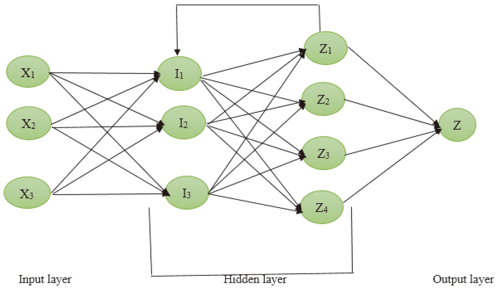

3.3 ANFIS

ANFIS is a worldwide estimator which helps in approximating whichever genuine incessant function having a solid set of accurateness level to any extent. Fundamental arrangement of FIS category is observed to be a model which helps mapping input characteristic to input membership functions (MFs). Subsequently it communicates this MF to rules and rules to a series of output characteristic. At last mapping of output characteristic to output MFs, and output MF into a solitary output or a conclusion linked with output [30, 31]. All FIS consists of three major components, defuzzifier, fuzzy database, and fuzzifier. Fuzzy rule base and deduction locomotive are two vital components of fuzzy database. Structure of an emblematic ANFIS is represented in Fig. 4. First layer comprises of nodes where each is an adapted one having a function namely generalized bell MF or a Gaussian MF. In second layer, each node is permanent on behalf of firing power of every regulation, and is evaluated using fuzzy and connective of ‘multiple’ of inward indicators. Each node in third layer is rigid on behalf of standardization firing power of every regulation. The $i^{\text{th}}$ node computes ratio of $i^{\text{th}}$ regulation’s firing power to summing up of two regulations firing powers. Each node in fourth layer is an adapted one having function representing involvement of $i^{\text{th}}$ regulation in direction of output on the whole. The solitary node in fifth layer is permanent node demonstrating complete output as summing up of all inward bound indicators [32].

Table 2
Performance of constraints using RNN

Scenario	Sigmoid function	Architecture	MSE		RMSE		R ${}^{2}$
			Training	Testing	Training	Testing	Training	Testing
Precipitation	Tan-sig	4-2-1	0.000618	0.000387	0.003651	0.002148	0.7815	0.8035
Avg. temperature		4-3-1	0.000714	0.000342	0.007385	0.004837	0.7691	0.7856
evapotranspiration		4-5-1	0.000376	0.000211	0.002745	0.003981	0.7237	0.7459
humidity		4-7-1	0.000553	0.000416	0.006384	0.008432	0.7529	0.7793
		4-9-1	0.000386	0.000129	0.005284	0.007129	0.7348	0.7577
	Log-sig	4-2-1	0.000365	0.000213	0.004416	0.005072	0.7946	0.8109
		4-3-1	0.000183	0.000088	0.003482	0.008176	0.7518	0.7739
		4-5-1	0.000552	0.000329	0.002771	0.007628	0.8026	0.8225
		4-7-1	0.000409	0.000239	0.005175	0.004827	0.7624	0.7921
		4-9-1	0.000624	0.000442	0.004428	0.005518	0.7405	0.7614
	Purelin	4-2-1	0.000723	0.000515	0.007183	0.006183	0.7155	0.7462
		4-3-1	0.000385	0.000129	0.006832	0.002218	0.7449	0.7623
		4-5-1	0.000426	0.000312	0.005931	0.004821	0.7001	0.7249
		4-7-1	0.000617	0.000404	0.007638	0.006739	0.7527	0.7735
		4-9-1	0.000558	0.000365	0.008235	0.001876	0.7328	0.7509

Table 3

Performance of constraints using ANFIS

Scenario	Membership function	MSE		RMSE		R ${}^{2}$
		Training	Testing	Training	Testing	Training	Testing
Precipitation	Pi	0.065845	0.173592	0.084765	0.214876	0.8007	0.8301
Avg. temperature	Tri	0.062765	0.163965	0.082764	0.215375	0.7347	0.7656
evapotranspiration	Trap	0.062859	0.153976	0.084846	0.210845	0.8756	0.7869
humidity	Gauss	0.060961	0.081276	0.083851	0.106398	0.7843	0.8116
	Gbell	0.050745	0.073972	0.070274	0.095731	0.8238	0.8514
	Gauss2	0.057658	0.088274	0.082358	0.139517	0.7628	0.7996

Table 4

Performance of constraints using RBFN

Scenario	Architecture	MSE		RMSE		R ${}^{2}$
		Training	Testing	Training	Testing	Training	Testing
Precipitation	5-0.2-1	0.00406	0.00331	0.3429	0.2418	0.7669	0.7927
Avg. temperature	5-0.3-1	0.00528	0.00409	0.4217	0.3169	0.7248	0.7528
evapotranspiration	5-0.5-1	0.00485	0.00248	0.04866	0.02747	0.7917	0.8109
humidity	5-0.7-1	0.00218	0.0107	0.7528	0.5502	0.7664	0.7992
infiltration loss	5-0.9-1	0.00601	0.00418	0.04984	0.03116	0.8201	0.8375

Figure 4.

Architecture of ANFIS.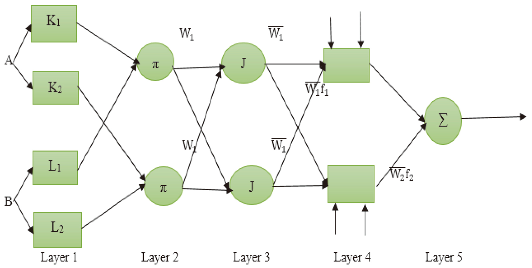

3.4 Model formulation and evaluation

Here two scenarios are considered to evaluate the performance of model. Monthly Precipitation, Avg. temperature, evapotranspiration, humidity are recommended as input parameter for scenario 1. Addition of infiltration loss with the parameters of scenario 1 is considered as input constraints for scenario 2. Data from 1994–2013 and 2014–2018 are used for training and testing network.

$\displaystyle R^{2}=1-\frac{{\left[\sum\limits^{N}_{i=1}{(x^{i}_{\textit{comp}% }-{\overline{x}}^{i}_{\textit{comp}})}\right]}^{2}}{{\left[\sum\limits^{N}_{i=% 1}{(x^{i}_{\textit{obs}}-{\overline{x}}_{\textit{obs}})}\right]}^{2}}$ (1) $\displaystyle\textit{MSE}=\frac{1}{N}\sum\limits^{N}_{j=1}{{(x^{i}_{\textit{% comp}}-x^{i}_{\textit{obs}})}^{2}}$ (2)

where, $x^{i}_{\textit{comp}}$ and $x^{i}_{\textit{obs}}$ are the computed and actual data.

${\overline{x}}^{i}_{\textit{comp}}$ and $x^{i}_{\textit{obs}}$ are the mean values of computed and measured data

Table 5

Performance of constraints using RNN

Model input	Sigmoid function	Architecture	MSE		RMSE		R ${}^{2}$
			Training	Testing	Training	Testing	Training	Testing
Precipitation	Tan-sig	5-2-1	0.000603	0.003748	0.018746	0.016384	0.9083	0.9235
Avg. temperature		5-3-1	0.000668	0.007183	0.022847	0.012843	0.8771	0.8937
evapotranspiration		5-5-1	0.000399	0.009246	0.031883	0.028437	0.8268	0.8457
humidity		5-7-1	0.000476	0.005147	0.049854	0.044265	0.8558	0.8701
infiltration loss		5-9-1	0.000775	0.004769	0.078432	0.074181	0.8113	0.8223
	Log-sig	5-2-1	0.000589	0.003152	0.020517	0.018824	0.8853	0.9117
		5-3-1	0.000698	0.007634	0.085379	0.083278	0.8335	0.8568
		5-5-1	0.000776	0.007843	0.044692	0.042746	0.9210	0.9476
		5-7-1	0.000837	0.009957	0.085178	0.083245	0.8558	0.8863
		5-9-1	0.000443	0.005306	0.077931	0.075847	0.8004	0.8382
	Purelin	5-2-1	0.000227	0.004478	0.062749	0.059374	0.7589	0.7638
		5-3-1	0.000625	0.008856	0.058312	0.054386	0.8365	0.8554
		5-5-1	0.000719	0.009315	0.084653	0.080012	0.7882	0.8001
		5-7-1	0.000482	0.006827	0.096125	0.093274	0.8749	0.8962
		5-9-1	0.000331	0.006639	0.073184	0.069025	0.8105	0.8337

Table 6

Performance of constraints using ANFIS

Scenario	Membership function	MSE		RMSE		R ${}^{2}$
		Training	Testing	Training	Testing	Training	Testing
Precipitation	Pi	0.059943	0.041482	0.072176	0.059273	0.9381	0.9658
Avg. temperature	Tri	0.062271	0.151876	0.085198	0.068162	0.8532	0.8873
evapotranspiration	Trap	0.050265	0.048821	0.070043	0.063871	0.8715	0.9036
humidity	Gauss	0.060316	0.055286	0.083964	0.080328	0.9146	0.9335
Infiltration loss	Gbell	0.057528	0.051987	0.077219	0.074182	0.9439	0.9676
	Gauss2	0.067187	0.062852	0.064281	0.060128	0.8933	0.9115

4. Results and discussions

4.1 Scenario 1

For RBFN results are conferred below for Nuapada station. For performance evaluation, 4-0.3-1, 4-0.2-1, 4-0.5-1, 4-0.9-1, and 4-0.7-1 architectures are deliberated. Preeminent model architecture is institute to be 4-0.5-1 which possesses MSE testing, training value 0.05894, 0.00509, RMSE testing, training value 0.07006, 0.06338 and R ${}^{2}$ testing, training value 0.7936, 0.7516. Details of performance are presented in Table 1.

Similarly, here to evaluate model altered transfer functions like logarithmic and tangential sigmoidal are engaged to illustrate model performance. R ${}^{2}$ , RMSE, MSE are evaluated for each architecture presented in Table 2. For all function in RNN, 4-7-1, 4-3-1, 4-2-1, 4-9-1, 4-5-1 architectures are applied for estimation of performance. For Tan-sig function finest model architecture is found to be 4-2-1 which possess MSE training, testing value 0.000618, 0.000387, RMSE training, testing value 0.003651, 0.002148 and R ${}^{2}$ for training, testing is 0.7815, 0.80355. For Log-sig function superlative model architecture is found to be 4-5-1 which possess MSE training, testing value 0.000552, 0.000329, RMSE training, testing value 0.002771, 0.007628 and R ${}^{2}$ for training, testing is 0.8026, 0.8225. The inclusive consequences are available in Table 3.

Six different membership functions are used to evaluate the efficacy of model in case of ANFIS algorithms. Among them Gbell function gives prominent value of performance which possess MSE and R ${}^{2}$ for training, testing value is 0.050745, 0.073972 and 0.8238, 0.8514.

Figure 5.

Actual verses predicted water table depth using ANFIS, RNN, and RBFN for (a) training and (b) testing phase.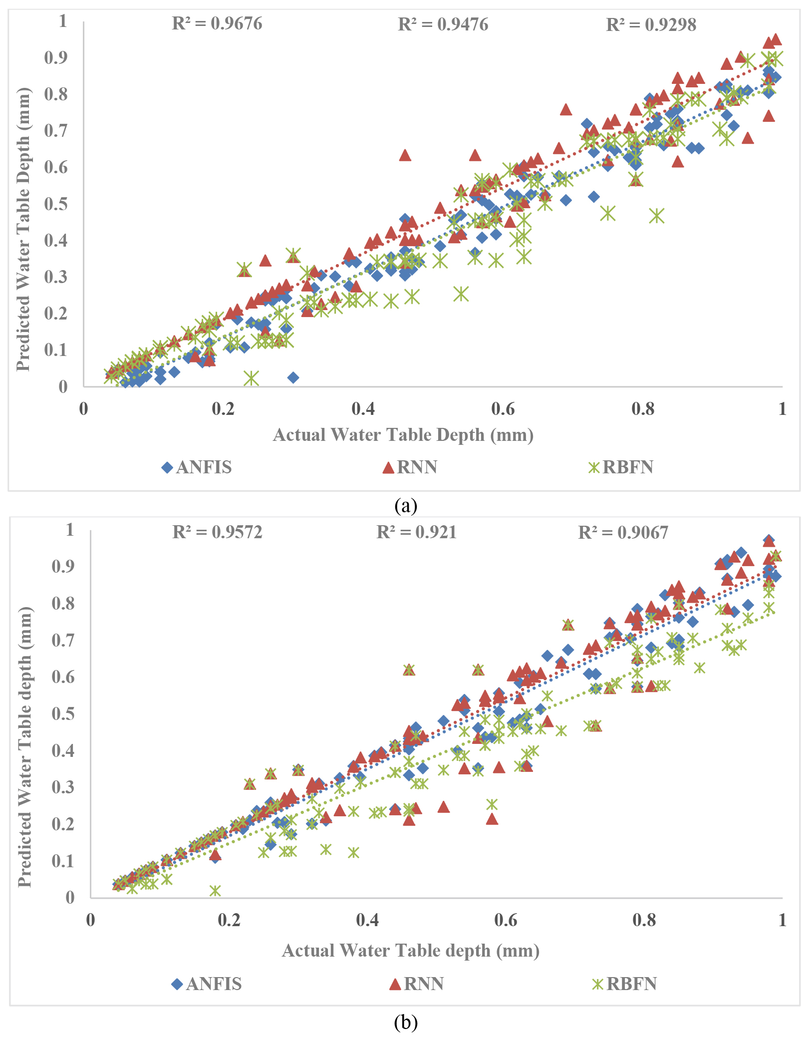

4.2 Scenario 2

Similarly for RBFN superlative model architecture is established to be 5-0.9-1 which retains MSE training, testing value 0.00601, 0.00418, RMSE training, testing value 0.04984, 0.03116 and R ${}^{2}$ for training, testing 0.8201, 0.8375. In case of RNN Log-sig function the best model architecture is found to be 5-5-1 which possess MSE training, testing value 0.000776 0.007843, RMSE training, testing value 0.044692, 0.042746 and R ${}^{2}$ for training, testing is 0.9210, and 0.9476. Gbell function gives best value of performance while ANFIS algorithm is used to develop model, which possess coefficient of determination 0.9439 and 0.9676 for training and testing phase respectively. A compressive detail of performance is presented in Tables 4–6 for RBFN, RNN, ANFIS algorithms.

Actual verses predicted water table depth using RBFN, RNN, and ANFIS for Scenario 2 are presented in Fig. 5.

5. Conclusion

Present study focuses on working application of three developments in ANN technique, i.e. ANFIS, RNN and RBFN model for comparing GL prediction in Nuapada watershed. Two scenarios are considered for evaluating efficacy of model. Inclusion of infiltration loss as input in context to scenario 1, model gives prominent performance. Model performance is done on basis of RMSE, MSE and R ${}^{2}$ . For RNN Log-sig function paramount model architecture is found to be 4-5-1 which retains testing and training value 0.007843, 0.000776 and coefficient of determination for training, testing value 0.9210, 0.9476. In case of ANFIS, Coefficient of determination for training and testing phase is 0.9439 and 0.9676. Among three techniques RBFN gives poor performance value with R ${}^{2}$ value is 0.8201 and 0.8375 for training and testing phase respectively. It can be seen that ANFIS performs relatively satisfying, giving better results than RBFN when performance trials are considered for present research. It is envisioned that ANFIS runs as an enhanced alternative tool to model groundwater process. Studies carried out on usability of ANFIS and RBFN for different aspects of hydrology shows that these models fit well for forecasting these aspects as in present study for groundwater level forecasting.

References

Yan

and Ma

, Application of integrated ARIMA and RBF network for groundwater level forecasting, Environmental Earth Sciences 75(5) (2016), 396.

Soleymani

S.A.

Goudarzi

Anisi

M.H.

Hassan

W.H.

Idris

M.Y.I.

Shamshirband

Noor

N.M.

and Ahmedy

, A novel method to water level prediction using RBF and FFA, Water Resources Management 30(9) (2016), 3265–3283.

Amutha

and Porchelvan

, Seasonal prediction of groundwater levels using ANFIS and radial basis neural network, International Journal of Geology, Earth and Environmental Sciences 1(1) (2011), 98–108.

Yin

J.C.

Zou

Z.J.

and Xu

, Sequential learning radial basis function network for real-time tidal level predictions, Ocean Engineering 57 (2013), 49–55.

Samantaray

Sahoo

and Ghose

D.K.

, June Assessment of Groundwater Potential Using Neural Network: A Case Study. In International Conference on Intelligent Computing and Communication, Springer, Singapore, 2019, pp. 655–664.

Daliakopoulos

I.N.

Coulibaly

and Tsanis

I.K.

, Groundwater level forecasting using artificial neural networks, Journal of hydrology 309(1-4) (2005), 229–240.

Affandi

A.K.

and Watanabe

, Daily groundwater level fluctuation forecasting using soft computing technique, Nature and Science 5(2) (2007), 1–10.

Coulibaly

Anctil

Aravena

and Bobée

, Artificial neural network modeling of water table depth fluctuations, Water Resources Research 37(4) (2001), 885–896.

Krishna

Satyaji

Y.R.

and Vijaya

, Modelling groundwater levels in an urban coastal aquifer using artificial neural networks, Hydrological Processes: An International Journal 22(8) (2008), 1180–1188.

10.

Emamgholizadeh

Moslemi

and Karami

, Prediction the groundwater level of bastam plain (Iran) by artificial neural network (ANN) and adaptive neuro-fuzzy inference system (ANFIS), Water Resources Management 28(15) (2014), 5433–5446.

11.

Suryanarayana

Sudheer

Mahammood

and Panigrahi

B.K.

, An integrated wavelet-support vector machine for groundwater level prediction in Visakhapatnam, India, Neurocomputing 145 (2014), 324–335.

12.

Moosavi

Vafakhah

Shirmohammadi

and Behnia

, A wavelet-ANFIS hybrid model for groundwater level forecasting for different prediction periods, Water Resources Management 27(5) (2013), 1301–1321.

13.

Jalalkamali

and Jalalkamali

, Groundwater modeling using hybrid of artificial neural network with genetic algorithm, African Journal of Agricultural Research 6(26) (2011), 5775–5784.

14.

Güldal

, and Tongal

, Comparison of recurrent neural network, adaptive neuro-fuzzy inference system and stochastic models in Eğirdir Lake level forecasting, Water Resources Management 24(1) (2010), 105–128.

15.

Yarar

Onucyıldız

and Copty

N.K.

, Modelling level change in lakes using neuro-fuzzy and artificial neural networks, Journal of Hydrology 365(3-4) (2009), 329–334.

16.

Chang

F.J.

and Chang

Y.T.

, Adaptive neuro-fuzzy inference system for prediction of water level in reservoir, Advances in Water Resources 29(1) (2006), 1–10.

17.

Coppola

E.A.

, Jr. Rana

A.J.

Poulton

M.M.

Szidarovszky

and Uhl

V.W.

, A neural network model for predicting aquifer water level elevations, Groundwater 43(2) (2005), 231–241.

18.

Sun

Wendi

Kim

D.E.

and Liong

S.Y.

, Application of artificial neural networks in groundwater table forecasting – a case study in a Singapore swamp forest, Hydrology and Earth System Sciences 20(4) (2016), 1405–1412.

19.

Firat

and Güngör

, River flow estimation using adaptive neuro fuzzy inference system, Mathematics and Computers in Simulation 75(3-4) (2007), 87–96.

20.

Samantaray

Sahoo

and Ghose

D.K.

, Assessment of runoff via precipitation using neural networks: watershed modelling for developing environment in arid region, Pertanika J Sci Technol 27(4) (2019), 2245–2263.

21.

and Mathur

, Modeling uncertainty analysis in flow and solute transport model using adaptive neuro fuzzy inference system and particle swarm optimization, KSCE Journal of Civil Engineering 14(6) (2010), 941–951.

22.

Karaboga

and Kaya

, Adaptive network based fuzzy inference system (ANFIS) training approaches: a comprehensive survey, Artificial Intelligence Review 52(4) (2018), 1–31.

23.

Sahoo

Samantaray

and Ghose

D.K.

, Stream flow forecasting in Mahanadi River Basin using artificial neural networks, Procedia Computer Science 157 (2019), 168–174.

24.

Nguyen

P.K.T.

Chua

L.H.C.

Talei

and Chai

Q.H.

, Water level forecasting using neuro-fuzzy models with local learning, Neural Computing and Applications 30(6) (2018), 1877–1887.

25.

Seo

Kim

Kisi

and Singh

V.P.

, Daily water level forecasting using wavelet decomposition and artificial intelligence techniques, Journal of Hydrology 520 (2015), 224–243.

26.

Gong

Zhang

Lan

and Wang

, A comparative study of artificial neural networks, support vector machines and adaptive neuro fuzzy inference system for forecasting groundwater levels near Lake Okeechobee, Florida, Water Resources Management 30(1) (2016), 375–391.

27.

Ansong

M.O.

Yao

H-X.

and Huang

J.S.

, Radial and sigmoid basis function neural networks in wireless sensor routing topology control in underground mine rescue operation based on particle swarm optimization, International Journal of Distributed Sensor Networks 9(9) (2013), 1–14.

28.

Xie

Paszczynski

and Wilamowski

B.M.

, Advantages of radial basis function networks for dynamic system design, Industrial Electronics, IEEE Transactions, 58(12) (2011), 5438–5450.

29.

Aqil

Kita

Yano

and Nishiyama

, Neural networks for real time catchment flow modeling and prediction, Water Resour Manag 21 (2007), 1781–1796.

30.

Jang

J.S.R.

Sun

C.T.

and Mizutani

, Neuro-fuzzy and soft computing: a computational approach to learning and machine intelligence, Prentice-Hall, Eaglewood Cliffs, 1997, pp. 665–685.

31.

Das

U.K.

Samantaray

Ghose

D.K.

and Roy

, Estimation of aquifer potential using BPNN, RBFN, RNN, and ANFIS. In Smart Intelligent Computing and Applications, Springer, Singapore, 2019, pp. 569–576.

32.

Jang

J.S.R.

and Sun

C.T.

, Neuro-fuzzy modeling and control, Proc IEEE 83 (1995), 378–406.

Modelling response of infiltration loss toward water table depth using RBFN,RNN,ANFIS techniques

Abstract

Keywords

1. Introduction

2. Case study

3.1 RBFN

Table 1 Performance of constraints using RBFN

Table 2 Performance of constraints using RNN

4.1 Scenario 1

5. Conclusion

References

Table 1
Performance of constraints using RBFN

Table 2
Performance of constraints using RNN