District level poverty estimation for rural Odisha (India) using different estimation techniques

Abstract

This paper examines the extent of poverty in different districts (small domains) of the State of Odisha, India using direct, synthetic, composite, and model based small area estimation techniques. The district level poverty estimates are based on data collected during the 68 ${}^{\rm th}$ round survey (2011–12) of the National Sample Survey Office (NSSO) and 2011 Population Census of India. It is shown that the model-based district level estimates are reasonably more reliable compared to other methods under comparison as confirmed by the diagnostic procedures.

Keywords

Poverty line NSSO household consumer expenditure survey population census and small area estimation

1. Introduction

Odisha is the tenth largest State in the Indian Union located on the eastern coast of the country bordered in the east by the Bay of Bengal. The geographical boundary of the State comprises 4.74% of India’s land mark, having population of 41.97 million as per 2011 Census, out of which 83.31% live in rural areas. Administratively Odisha has been divided into 3 Revenue Divisions, 30 Districts and 314 Community Development Blocks. Odisha is a land of diversities and inhabited by different ethnic groups. About 40% of the population of the State belong to backward communities like the Scheduled Caste (17.1%) and the Scheduled Tribe (22.8%) communities. The per capita income (Net State Domestic Product (NSDP)) of Odisha during 2014–15 is estimated at Rs. 28, 384.00 (approximately 435 USA Dollars) indicating a growth rate of 7.3% over 2013-14 which is well below the National figure.

Agriculture is the major source of income of the rural Odisha accounting to 15.5% of Gross State Domestic Product (GSDP) as per advance estimate 2016–17. The vagaries of nature exposed to the State’s agriculture sector economy frequently cause cyclones, droughts and flash floods which substantially affect the production and productivity of agriculture. In spite of rich cultural heritage and being endowed with abundant natural resources e.g. minerals, forests, rivers etc. and long coast line and favourable political and social climate, Odisha stands at the bottom of the economic development as compared to most of the states of the country.

As per the World Bank Reports (2016) the districts of Odisha in the south and west are among the poorest in the country and the State. The coastal districts are economically more developed than other districts of the State. There is also widening gap between the rich and the poor across the social groups as well as across the regions.

Inputs on different socio-economic characteristics at grass root level like district, block etc. are highly essential for decentralised planning and strategies for programme implementation to handle the backward areas of the State. Certain items of information such as consumer expenditure/income data essential for grass-root planning are not covered in the population census schedules. Besides, conduct of the decennial census in India, the National Sample Survey Office (NSSO) carries out country wide surveys in India on various socio-economic parameters related to the national economy on varied topics as per demand of the Government of India from time to time in a regular basis in the form of different rounds during the inter-censal periods. The sample sizes so designed for the surveys of the NSSO are modest in nature and are fixed in such a way that it is possible to get some usable estimates at the national and state level. However, due to the importance of micro level planning in a developing country like India, where there is large scale poverty in most parts of the country, reliable estimates are being demanded by the administrators and policy planners at the small area level as per the recommendations of “Working Group on District Planning” set up by the Planning Commission of the Government of India during 1982. The Working Group in its report clearly highlighted the data requirement for planning and decision making at the district level. The sample sizes in NSSO surveys at the State level are not large enough to provide reliable direct estimates at small area level like district level, block level, community level etc. Conduct of district specific surveys with large sample also becomes expensive as well as time consuming.

During recent years in view of the demand for reliable statistics at micro level, Small Area (domain) Estimation (SAE) techniques have been developed to produce reliable estimates for such small areas with small sample sizes by borrowing strength from data relating to other areas through explicit and implicit models which connect the small areas via supplementary data (Rao, 2003). Typically, small area in our study refers to a subset of the population for which enough information is not available from the sample survey because of limited sample size. This creates problems to derive reliable estimates of small geographical areas like districts.

The main objective of the study is to estimate the rural poverty in Odisha at district levels based on the 68 ${}^{\rm th}$ round (2011–12) of the Household Consumer Expenditure data of the National Sample Survey Office (NSSO) and the Indian Population Census (2011) data, using direct, indirect, and small area estimation techniques and to make comparison among them as regards their reliabilities.

2. Data

The data have been collected from the Population Census, 2011 and the Household Consumer Expenditure Survey, 2011–12 of the NSSO (68 ${}^{\rm th}$ Round) for the rural area of Odisha, which provides data on Monthly Per Capita Expenditure (MPCE). The data on covariates (auxiliary variables) collected from the Population Census, 2011 are total population, Scheduled Caste (SC) population, Schedules Tribe (ST) population, male population, female population, sex ratio, child sex ratio, male literacy, female literacy, SC literacy, ST literacy, Work Participation Rate (WPR), female WPR etc.

3. Sampling design

The sampling design used in the 68 ${}^{\rm th}$ round NSSO survey for the year 2011–12 is stratified multistage random sampling with districts as strata, villages as fist stage units (FSU) and households as the second stage units (SSU). During the 68 ${}^{\rm th}$ round NSSO survey, a total 2973 households were surveyed from 30 districts of Odisha comprising 96, 91,085 households (2011 Census). The district wise rural sample size varied from 64 to 128 with average sample size of 99 (Table 1).

Table 1
Distribution of districts-wise rural sample size

Sl No.	District name	No. of households	Sl No.	District name	No. of households
1	Angul	95	16	Kandhamal	64
2	Balasore	128	17	Kendrapara	126
3	Baragarh	128	18	Keonjhar	128
4	Bhadrak	128	19	Khurda	96
5	Bolangir	96	20	Koraput	96
6	Boudh	64	21	Malkangiri	64
7	Cuttack	128	22	Mayurbhanja	128
8	Deogarh	64	23	Nawrangapur	96
9	Dhenkanal	96	24	Nayagarh	96
10	Gajapati	64	25	Nuapada	64
11	Ganjam	160	26	Puri	128
12	Jagatsinghpur	96	27	Rayagada	64
13	Jajpur	128	28	Sambalpur	64
14	Jharsuguda	64	29	Sonepur	64
15	Kalahandi	128	30	Sundargarh	128
16	Kandhamal	64		Odisha	2973

4. Poverty line

The poverty line for identifying whether a given household is poor or not, is fixed by the Planning Commission of the Government of India as per the methodology adopted by an Expert Group headed by Prof. Suresh Tendulkar at the National level in 2009. For rural Odisha the poverty line is fixed at Rs. 695.00 (roughly equivalent to 10.80 USA dollars). Monthly Per Capita Expenditure for the year 2011–12 is defined as the minimum or the cut off standard of expenditure on food below which an individual or household is described as poor. State level rural poverty lines were calculated from the National level poverty line by applying appropriate regional price indices.

As such, a single State level official poverty line for Odisha as recommended by the Planning Commission, Government of India has been used. The poverty estimation carried out for the districts of the Odisha State has not taken into account the different administrative efficiencies, available natural resources, infrastructural facilities, and political initiatives because of lack of required quantitative indicators. It may be mentioned here that the current poverty analysis of the NSSO consumer expenditure data is based on samples, assumed to be selected by simple random sampling (without replacement) from the population of households in the country, although the samples have been selected at different stages. This is done in order to simplify the mathematical complexities involved in the estimation and to provide a reasonably good approximation for the purpose for which it is supposed to be applied.

5. Methods of estimation of poverty

The district wise poverty estimation has been carried out by (i) Direct Method (ii) Indirect/Synthetic Method, (iii) Composite Method, and (iv) Small Area Estimation (SAE) technique using mixed model approach.

5.1 Direct method

Let $U=\{1,2,3,\ldots,N\}$ be the finite population of size $N$ consisting of $D$ disjoint sub-population or small areas $U_{i}$ each with sub-population size $N_{i}(i=1,2,\ldots,D)$ such that $U=\operatorname*{\cup}\limits_{i=1}^{D}\cup_{i}$ , and $N=\sum\nolimits_{i=1}^{D}N_{i}$ . Assume that a sample $s$ of size $n$ is selected with simple random sampling without replacement (SRSWOR) out of finite population of size $N$ .

Define $\pi_{j}(j=1,2,3,\ldots,N)$ as the first order inclusion probability for the element $j$ and $w_{j}=\frac{1}{\pi_{j}}$ as the design weight of the element $j$ . Under the simple random sampling $\pi_{j}=\frac{n}{N}$ and $w_{j}=\frac{1}{\pi_{j}}=\frac{1}{n/N}=\frac{N}{n}$ .

Let $s_{i}$ be the part of the sample $s$ of size $n_{i}(n_{i}\geqslant 0)$ that falls in small area $i$ . Then $n=\sum\nolimits_{i=1}^{D}n_{i}$ . Let $y$ be the characteristic under study. Denote $Y_{ij}$ as the value of $y$ for the $j^{\rm th}$ population unit of the $i^{\rm th}$ small area unit. Define the population mean of the $i^{\rm th}$ small area as

$\bar{Y}_{i}=\sum\limits_{j\in Ui}Y_{ij}/N_{i}∼{}∼{}(i=1,2,3,\ldots\ldots,D).$

Let $y_{ij}$ be the value of $y$ of the $j^{\rm th}$ household of the $i^{\rm th}$ small area (in the present case it is district) ( $i=1,2,3,\ldots,D$ ), where $D=$ 30, being the number of districts of the State of Odisha (India) where $y_{ij}=1$ for household below poverty line and $y_{ij}=0$ otherwise. Under the simple random sampling (SRS) without replacement, a direct estimator of the population mean $\bar{Y}_{i}$ /population proportion for the $i^{\rm th}$ domain is given by $\hat{p}_{i}^{d}=\hat{\bar{Y}}_{i}^{d}=\frac{\sum\nolimits_{si}{W_{j}y_{j}}}{% \sum W_{j}}=\frac{\sum y_{j}}{n_{i}}$ with variance $\textit{Var}(\hat{\bar{Y}}_{i}^{d})=\left(1-f_{i}\right)S_{i}^{2}{/n}_{i}$ , where ${f}_{i}=\frac{n_{i}}{N_{i}}$ and

$S_{i}^{2}=\frac{1}{\left(N_{i}-1\right)}\sum\nolimits_{j=1}^{N_{i}}\left(Y_{ij% }-\bar{Y}_{i}\right)^{2},i=1,2,\ldots,D$

An unbiased estimator of $S_{i}^{2}$ is $s_{i}^{2}=\frac{1}{\left(n_{i}-1\right)}\sum_{{j\in si}}{(y_{ij}-\bar{y}_{i})}% ^{2}$ .

The district level poverty estimation of Odisha for the rural sector is computed by head count method (direct estimation procedure) using the 68 ${}^{\rm th}$ round National Sample Survey (NSS) consumer expenditure data. The proportion of poor, standard error, co-efficient of variation (CV) and confidence interval (CI) using the direct method are presented in Table 2. The CVs are shown as the sampling variability as a percentage of the estimate.

Direct estimates are generally computed when the sample size for each small domain (small area) is sufficiently large to provide reasonably accurate estimates about the parameters of interest. However, when the data are collected to provide national and regional level statistics, the sample sizes for the sub-domains of the original domain happen to be usually very small leading to unacceptably large sampling variance.

An extension of direct estimation approach is to use the auxiliary information in the sample to arrive at more precise estimates for the small domains based on suitable regression technique (model-assisted approach to the design-based sampling theory). This improves the precision of direct estimates, but still affected by small sample sizes.

In the present study we have used direct method for estimation of proportion of households in poverty using log linear regression model. The unknown regression coefficients in the model can be estimated by the method of least squares using sample households, the population means of the auxiliary variables (usually unknown), may be used from either from recent census or from administrative official records or from other sources.

The covariates (auxiliary variables/independent variables) observed in NSSO sample survey used in regression analysis are household size, social group, total land possessed, primary source of lighting, primary source of cooking, salary earner, age, sex, marital status and general education of the head of the household, percentage of food in MPCE and household amenities etc. But only the effects of covariates such as household size, social group, total land possessed, primary source of lighting, salary earner, age, marital status, general education of the head of the household, percentage of food in MPCE are found to be significant, ascertained from the stepwise regression method of fitting the regression. The value of R ${}^{2}$ is computed to be 0.5082, which is found to be significant.

The district wise estimates of proportion of poverty along with standard error, CV and CI using headcount method and log linear regression model are shown in Table 2.

5.2 Indirect methods

As stated earlier, the sample size for each small area is usually very small the direct estimator does not seem to be reliable. Further, the associated standard errors of these estimates are likely to be very large and unreliable. Under such circumstances, it is required to devise estimation methods which borrow strength from the related areas. These estimators are known as the Indirect estimators since they use supplementary/explanatory variables from other small areas or times and possibly from both or from census. The usual indirect estimation techniques based on implicit models produce synthetic and composite estimators.

5.2.1 Synthetic estimators

Gonzalez (1973) described synthetic estimation as follows: “An unbiased estimate is obtained from a sample for large area; when this estimate is used to derive estimates for sub-areas on the assumption that the small areas have the same characteristics as the large area, we identify these estimates as synthetic estimates”. This method borrows strength from related subareas to increase the effective sample size for estimation and hence, the accuracy of the resulting estimates (Holt et al., 1979).

The method of synthetic estimation presupposes the availability of estimates from an inquiry or survey of estimates for a large subset of the population such as large geographical area (e.g. Country, State etc.) or demographic group (e.g. age group, sex group etc.) or social group (e.g. community, disability group, or an industrial group etc.). Appropriate weights are then applied to large population subset estimates to arrive the desired small area estimates. In certain studies censuses provide sources of their weights.

5.2.2 Matching variables in the survey and the census

Before modelling, it is essential to select the list of explanatory variables that exist both in the survey and the census. If the sample selected for the household survey is representative and randomly selected from the population, one can expect the distribution of the variables to be similar both in the survey and in the population. Initially, a list of common variables was constructed using both the census schedule (the house list schedule) and the household schedule of NSSO Consumer Expenditure survey. Due to non-availability of village directory from the census, the household level variables have been converted into village characteristics in both, the census and the survey data and then, the village level data is converted into district level and hence district level variables are generated to be used in the regression model. National Sample Survey (NSS) data do not contain any village/district level variables. As the location effects captured by the village/district level variables are important determinant of consumption behaviour in order to control for location effects, we rely only on village/district level variables that can be created from the available household level variables (Sisodia & Singh, 2001). But the covariates (explanatory variables) are available at districts level not below that level. So, the area level area model is adopted to derive the small area level estimates. These covariates are drawn from the census 2011. The relationship between variables of interest and covariates used in this study are assumed not to change significantly over the period. There were more than 100 covariates available from the population census for the purpose of modelling.

5.2.3 Selection of covariates

First, examine the correlation of all the available covariates with the target variable and then select the covariates with reasonably good correlation with the target variable. After the selection of covariates, the model can be estimated controlling for both the household and village level effects following the step-wise regression analysis. Covariates are retained in the model according to their statistical significance. The variables with low t-values are removed. So, the five variables like household size, ST percentage, SC percentage, Work Participation Rate (WPR), and female literacy rate were identified for further analysis which significantly explained the model.

The regression synthetic estimator of $\bar{Y}_{i}$ of the $i^{\rm th}$ small area is ( $i=1,2,\ldots D$ ) defined as

$\hat{\bar{Y}}_{i}^{\textit{synREG}}=\bar{y}_{i}+\hat{\beta}_{1}\left(\bar{X}_{% 1i}-\bar{x}_{1i}\right)+\hat{\beta}_{2}\left(\bar{X}_{2i}-\bar{x}_{2i}\right)+% \ldots+\hat{\beta}_{p}\left(\bar{X}_{pi}-\bar{x}_{pi}\right)$ (1)

where $\hat{\beta}_{1},\hat{\beta}_{2},\ldots,\hat{\beta}_{p}$ are full sample estimates calculated using sample data from entire area and thus different from the direct regression estimator. $\bar{X}_{1i},\bar{X}_{2i},\ldots,\bar{X}_{pi}$ are related to entire small area in the population census and $\bar{x}_{1i},\bar{x}_{2i},\ldots,\bar{x}_{pi}$ relate to small area in the sample.

5.2.4 Composite estimators

Ghosh and Rao (1994) suggested a weighted combination of the direct estimator and synthetic estimator to arrive at a composite estimator for the population total of $Y$ in $i^{\rm th}$ small area defined as:

$\hat{\bar{Y}}_{i}^{c}=w_{i}\hat{\bar{Y}}_{i}^{d}+\left(1-w_{i}\right)\hat{\bar% {Y}}_{i}^{\textit{synREG}}$ (2)

where $\hat{\bar{Y}}_{i}^{d}$ and $\hat{\bar{Y}}_{i}^{\textit{synREG}}$ are the direct estimator and synthetic estimator respectively and $w_{i}$ is an appropriately determined weight $\left(0\leqslant w_{i}\leqslant 1\right)$ .

Ghosh and Rao (1994) suggested to obtain optimal weights by minimizing the Mean Square Error (MSE) of $\hat{\bar{Y}}_{i}^{c}$ with respect to $w_{i}$ assuming that $cov\left(\hat{\bar{Y}}_{i}^{d},\hat{\bar{Y}}_{i}^{\textit{synREG}}\right)=0$ , which gives after estimating corresponding mean square error and variance.

$\hat{w}_{i}=\frac{\widehat{\textit{MSE}}\left(\hat{\bar{Y}}_{i}^{\textit{% synREG}}\right)}{\widehat{\textit{MSE}}\left(\hat{\bar{Y}}_{i}^{\textit{synREG% }}\right)+V\left(\hat{\bar{Y}}_{i}^{d}\right)}$

The composite estimator is expected to balance the potential bias of the synthetic estimator against the sustainability of the direct estimator. In the present study composite estimates for poverty at district level is obtained by combining direct estimate and the synthetic estimate giving weight as the inverse of root mean square error. Table 2 presents the district wise percentage of poverty using synthetic and composite estimates.

5.3 Model-based estimator

The traditional indirect estimator assumes that all the areas of interest behave similarly with reference to the variable of interest and do not take into account the area specific variability. This will lead to severe biasness if the assumption of homogeneity within the larger area is violated or the structure of the population changed since the previous census. This limitation is taken care up by an alternative estimation techniques based on an explicit linking model named as mixed effect model. Random area effects in the mixed effect model take into account of the dissimilarities among the areas.

Mixed models are used in specific situations based on data availability or the response variable of interest. These are (i) area level random effect models which use area specific auxiliary information and where information or response variable available only at the small area level (Fay & Herriot, 1979) and (ii) unit level regression models which uses the unit level auxiliary information and where information on the response variable is available at the unit level (Battese et al., 1988). In the absence of unit level data we resort to area level models.

5.3.1 Area level models

This model first conceived by Fay and Herriot (1979) was used for the prediction of mean per capita income in small geographical areas. An area level model based on two components:

Direct estimates of $\theta$ which is a function of finite population mean, based on the sampling design, given by

$\displaystyle\hat{\theta}_{i}=\theta_{i}+e_{i},∼{}∼{}i=1,2,\ldots,D$ (3)

where $e_{i}^{\prime}$ s are design-based errors assumed to independent across the small areas with $E(e_{i})=0$ and $V(e_{i})={\sigma}_{e}^{2}$ is a design-based sampling variance.

At linking model (Srivastava, 2016) is

$\displaystyle\theta_{i}=\bm{X}_{\bm{i}}\bm{{}^{\prime}}\bm{\beta}+u_{i},i=1,2,% \ldots,D$ (4)

where $\bm{\beta}$ is a $p$ -vactor unknown fixed effects and the random effect model error $u_{i}$ is assumed to be independent and identically distributed with mean zero and variance $\emptyset$ .

Combining these two models we finally obtain a linear mixed effect model given by

$\displaystyle\hat{\theta}_{i}=\bm{X}_{\bm{i}}\bm{{}^{\prime}}\bm{\beta}+u_{i}+% e_{i},∼{}∼{}i=1,2,\ldots,D$ (5)

Here $e_{i}^{\prime}$ s and $u_{i}^{\prime}$ s are design-based and model-based random variables respectively. The models variance $\emptyset$ is a measure of homogeneity of the areas after accounting for the covariates $X_{i}.$ Since the unknown parameters $\bm{\beta}$ and $\emptyset$ are the same for every area, there is reason to estimate $\bm{\beta}$ and $\emptyset$ across all $D$ areas.

In the present discussion $y$ represents the variable under study (the number of poor households). Define $y_{si}$ and $y_{ri}$ as the observed and non-observed part of poor households in area $i$ , $y_{si}$ has a binomial distribution B ( $n_{i,,}\pi_{i}$ ) and $y_{ri}$ has also a binomial distribution with distribution B ( $N_{i}-n_{i},\pi_{i}$ ). $\pi_{i}$ is the probability of success having a poor household in the area i. In the model used in the small area estimation is supplemented by auxiliary variables (co-variates) available from other sources such as census and official records.

The Fay and Herriot (FH) method for SAE is based on area level liner mixed model and their approach is applicable to a continuous variable. But for discrete, particularly binary variable, the model linking the probability of success $\pi_{i}$ with the covariates $X_{i}$ is the logistic linear mixed model given by

$\displaystyle\textit{Logit}∼{}\pi_{i}=\ln\left[\frac{\pi_{i}}{1-\pi_{i}}\right% ]=\bm{X}_{\bm{i}}\bm{{}^{\prime}}\bm{\beta}+u_{i},∼{}∼{}i=1,2,\ldots,D$ (6)

The expected values of $y_{si}$ and $y_{ri}$ given $u_{i}$ under model are

$\displaystyle E\left(y_{si}/u_{i}\right)=n_{i}\pi_{i}=n_{i}\left[\left(\exp{X_% {i}^{\prime}\bm{\beta}+u_{i}}\right)\left(1+\exp{(X_{i}^{\prime}}\bm{\beta}+u_% {i}\right)^{-1}\right]$ (7) $\displaystyle E\left(y_{ri}/u_{i}\right)=\left(N_{i}-n_{i}\right)\mathrm{}\pi_% {i}=\left(N_{i}-n_{i}\right)\left[\left(\exp{X_{i}^{\prime}\bm{\beta}+u_{i}}% \right)\left(1+\exp{(X_{i}^{\prime}}\bm{\beta}+u_{i}\right)^{-1}\right]$ (8)

Let $T_{i}$ denotes the total number of poor households in the district $d$ . We can write $T_{i}=y_{si}+y_{ri}$ where the first term $y_{si}$ the sample count is known where as the second term $y_{ri}$ the non-sample count, is unknown. Therefore, the estimate $\hat{T}_{i}$ of the total number of households in area $i$ is obtained by replacing $y_{ri}$ by its predicted value under the model is

$\hat{T}_{i}=y_{si}+\hat{y}_{ri}=y_{si}+\left(N_{i}-n_{i}\right)\left[(\exp{X_{% i}^{\prime}\hat{\bm{\beta}}+\hat{u}_{i}})(1+\exp(X_{i}^{\prime}\hat{\bm{\beta}% }+\hat{u}_{i})^{-1}\right]$ (9)

An estimate of proportion of poor households $p_{i}$ in small area $i$ is obtained as

$\hat{p}_{i}=\frac{\hat{T}_{i}}{N_{i}}=\frac{1}{N_{i}}\left\{y_{si}+\left(N_{i}% -n_{i}\right)\left[(\exp{X_{i}^{\prime}\hat{\bm{\beta}}+\hat{u}_{i}})(1+\exp(X% _{i}^{\prime}\hat{\bm{\beta}}+\hat{u}_{i})^{-1}\right]\right\}$ (10)

It is obvious that in order to compute the estimates given by the above two equations we require estimates of the unknown parameters $\bm{\beta}$ and $u$ . A major difficulty in use of logistic linear mixed model (LLMM) for SAE is the estimation of unknown model parameters $\bm{\beta}$ and $u$ since the likelihood function for LLMM often involves high dimensional integrals (computed by integrating a product of discrete and normal densities, which has no analytical solution) which are difficult to evaluate numerically. We used an interactive procedure that combines the Penalized Quasi-Likelihood (PQL) estimation of $\bm{\beta}$ and $u=(u_{1},\ldots,u_{D})$ with restricted maximum likelihood (REML) estimation of $\emptyset$ to estimate the parameters. (Saei & Chambers, 2003) and (Manteiga et al., 2007).

The estimation of mean squared error (MSE) for predictors given by Eq. (9). The MSE estimates are computed to assess the reliability of estimation and also to construct the confidence interval (CI) for the estimates. The mean squared error estimates of Eq. (9) under model (1) is given by

$\textit{mse}\left(\hat{p}_{i}\right)=m_{1}\left(\hat{\emptyset}\right)+m_{2}% \left(\hat{\emptyset}\right)+{2m}_{3}\left(\hat{\emptyset}\right)$ (11)

The first two components $m_{1}$ and $m_{2}$ constitute the largest part of the overall MSE estimates in Eq. (11). These are the MSE of the best linear unbiased predictor (BLUP) – type estimator when $\emptyset$ is known (Rao, 2003). The third component $m_{3}$ is the variability due to the estimate of $\emptyset$ .

In this study area level models which was used by Chandra et al. (2011) and Mantiga et al. (2007) have been applied for computing district level poverty estimates along with their mean square error estimates following the mathematically tedious developed by Prasad and Rao (1990), for which R-software packages version 3.3.0 are available.

5.3.2 Diagnostic procedures on model-based estimation (SAE)

The aim of the diagnostic procedures are used to validate the reliability of the model based small area estimates vrs direct survey estimates. Generally, two types of diagnostic procedures are used in SAE, ie. model diagnostics and small area estimates validation/diagnostics. The model diagnostics are used to verify the assumptions of underlying the model. The second diagnostics are used to validate the reliability of the model-based SAE. Model-based estimates should be consistent, more precise, more stable and acceptable.

Figure 1.

Biased scatter plot of the direct and model-based estimates.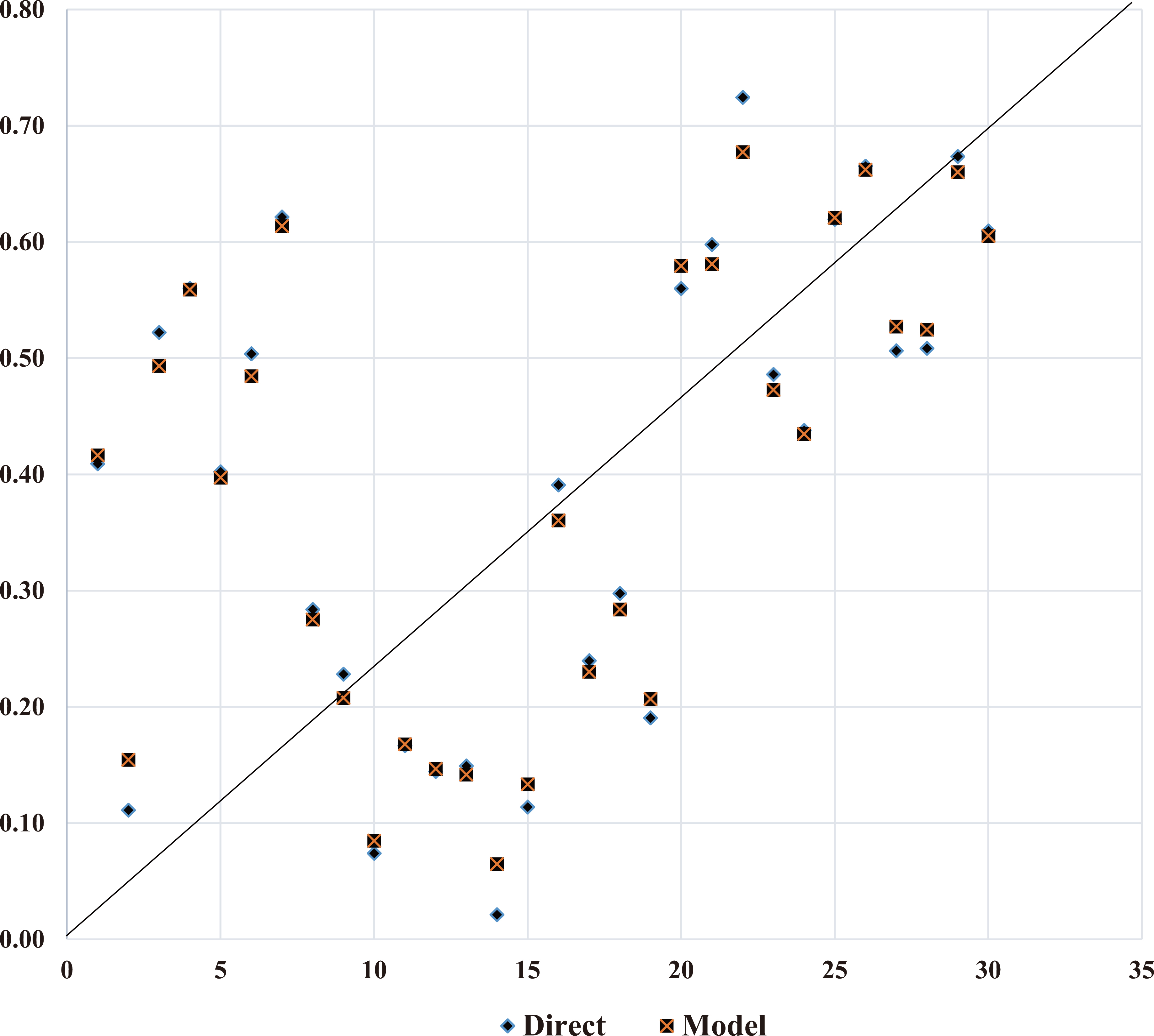

Figure 2.

District level residuals.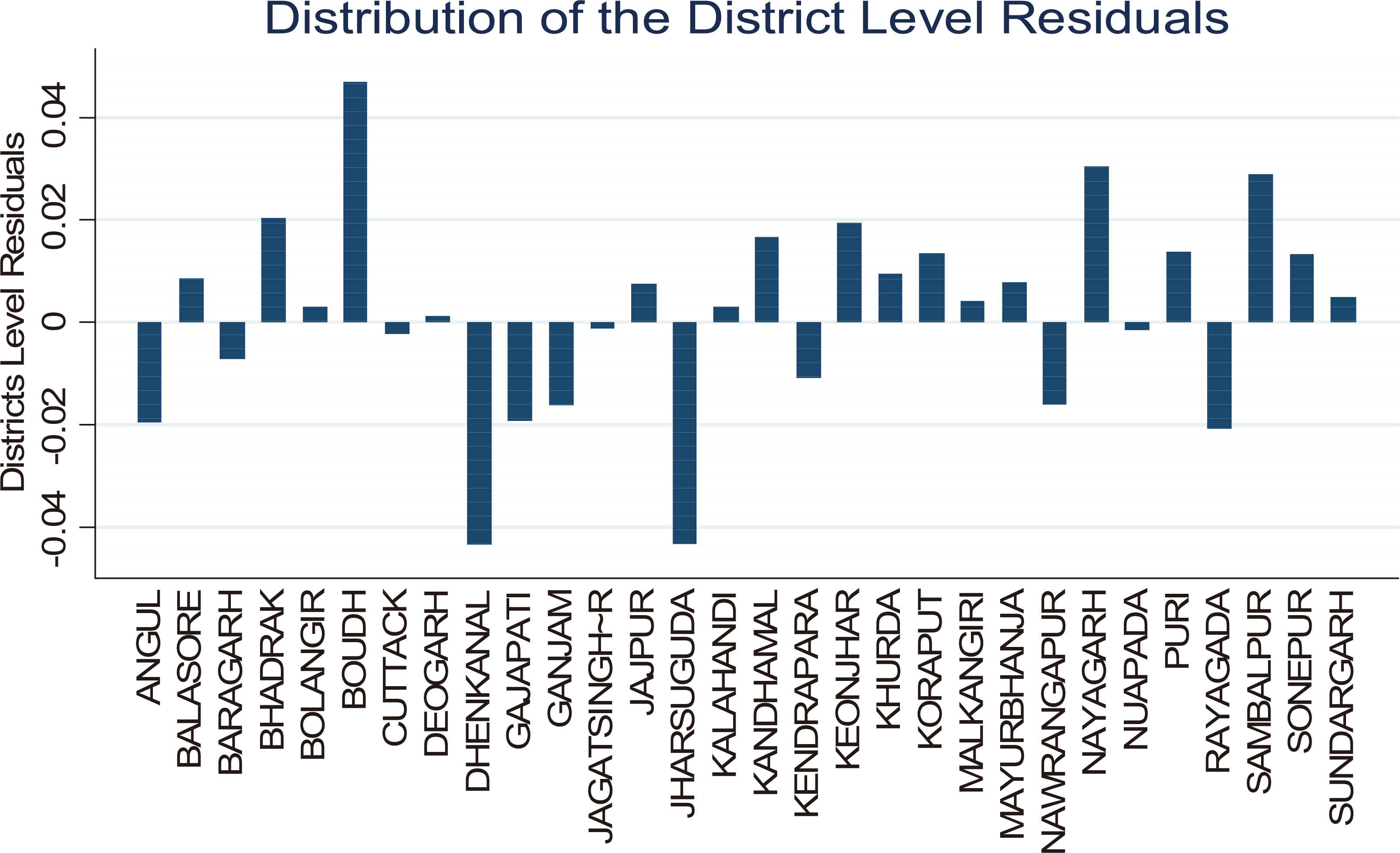

Figure 3.

q-q plot.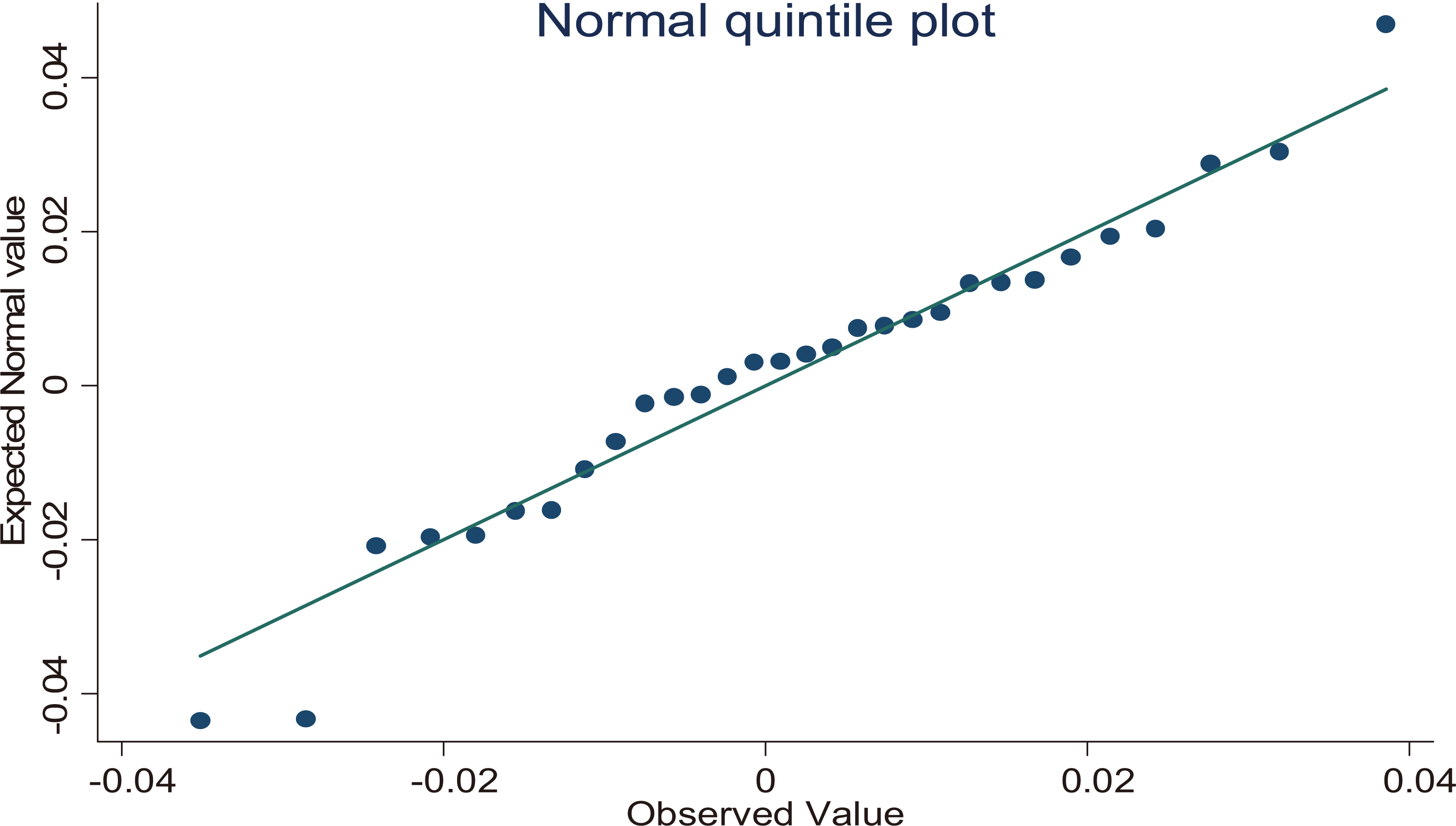

The bias diagnostics are used to assess the deviations of the model-based estimates from the direct survey estimates. The model-based estimates are expected to be biased predictors of the direct estimates. The model-based estimates will be unbiased predictors of the direct survey estimates if the relationship between the variable of interest and the covariates have been mis-specified or mis-estimated. Where, the relationship has not been mis-estimated, a linear relationship of the type $y=x$ is expected between the direct survey estimates and the model-based estimates. Figure 1 shows the biased scatter plot of the direct estimates against the model-based with the fitted regression line and the $y=x$ line. The plots show that the model-based estimates are less extreme as compared to the direct estimates. The distribution of the district level residuals and q-q plots are shown in Figs 2 and 3 respectively. This reveals that the randomly distributed district level residuals and the line of fit does not significantly differ from the line $y=0$ as expected in all the plots. The q-q plots also confirm the normality assumption. Therefore, the model diagnostics are fully satisfied for the data.

Table 2

Districtwise estimates of incidence of poverty, coefficient of variation and 95% confidence interval

Sl. No.	District	Direct				Direct (Predicted)				Synthetic
		Prop	CV (%)	95% Confidence		Prop	CV (%)	95% Confidence		Prop	CV (%)	95% Confidence
				interval				interval				interval
				Lower	Upper			Lower	Upper			Lower	Upper
1	Angul	0.11	46.14	0.01	0.22	0.07	37.18	0.04	0.10	0.16	34.10	0.11	0.22
2	Balasore	0.28	34.26	0.09	0.48	0.12	23.75	0.09	0.15	0.31	30.67	0.22	0.41
3	Baragarh	0.41	19.01	0.26	0.56	0.32	12.90	0.28	0.36	0.45	20.54	0.36	0.54
4	Bhadrak	0.23	24.97	0.12	0.34	0.17	19.67	0.13	0.20	0.28	34.54	0.18	0.37
5	Bolangir	0.44	20.42	0.26	0.61	0.27	16.74	0.23	0.32	0.37	17.41	0.30	0.43
6	Boudh	0.72	13.72	0.53	0.92	0.56	11.12	0.50	0.62	0.70	13.91	0.60	0.79
7	Cuttack	0.15	43.74	0.02	0.27	0.03	55.71	0.01	0.04	0.18	44.25	0.10	0.26
8	Deogarh	0.56	6.22	0.49	0.63	0.30	18.94	0.25	0.36	0.50	18.82	0.40	0.59
9	Dhenkanal	0.02	68.69	$-$ 0. 01	0.05	0.29	15.86	0.25	0.34	0.03	167.54	$-$ 0.02	0.09
10	Gajapati	0.56	27.83	0.25	0.87	0.40	15.32	0.34	0.46	0.40	31.54	0.28	0.53
11	Ganjam	0.19	30.94	0.08	0.31	0.29	12.53	0.25	0.32	0.24	27.80	0.18	0.31
12	Jagatsinghpur	0.17	29.72	0.07	0.26	0.22	19.34	0.18	0.26	0.24	29.61	0.17	0.31
13	Jajpur	0.15	30.58	0.06	0.24	0.09	28.40	0.06	0.11	0.21	34.45	0.13	0.28
14	Jharsuguda	0.11	54.08	$-$ 0.01	0.23	0.24	22.17	0.19	0.29	0.02	48.89	0.01	0.03
15	Kalahandi	0.67	10.07	0.53	0.80	0.36	11.82	0.32	0.40	0.60	10.27	0.54	0.66
16	Kandhamal	0.60	29.24	0.25	0.94	0.58	10.67	0.52	0.64	0.46	30.28	0.32	0.60
17	Kendrapara	0.07	66.44	$-$ 0.02	0.17	0.09	28.61	0.06	0.11	0.14	49.10	0.07	0.21
18	Keonjhar	0.50	18.67	0.32	0.69	0.55	8.07	0.50	0.59	0.41	19.72	0.33	0.49
19	Khordha	0.24	33.10	0.08	0.40	0.20	20.17	0.16	0.24	0.23	33.05	0.15	0.30
20	Koraput	0.67	11.65	0.52	0.83	0.23	18.91	0.18	0.27	0.38	28.05	0.28	0.49
21	Malkangiri	0.61	22.33	0.34	0.88	0.17	27.66	0.12	0.22	0.50	35.59	0.32	0.67
22	Mayurbhanja	0.62	12.96	0.46	0.78	0.48	9.13	0.44	0.53	0.41	32.25	0.28	0.54
23	Nawrangapur	0.51	13.49	0.37	0.64	0.49	10.32	0.44	0.55	0.45	27.05	0.33	0.57
24	Nayagarh	0.39	19.72	0.24	0.54	0.28	16.48	0.23	0.32	0.32	28.73	0.23	0.42
25	Nuapada	0.62	18.93	0.39	0.85	0.52	12.08	0.45	0.58	0.55	17.82	0.45	0.64
26	Puri	0.30	27.87	0.14	0.46	0.06	33.79	0.04	0.09	0.33	29.32	0.23	0.43
27	Rayagada	0.51	23.19	0.28	0.74	0.20	25.10	0.15	0.25	0.26	53.50	0.12	0.39
28	Sambalpur	0.52	21.81	0.30	0.75	0.41	14.95	0.35	0.47	0.52	20.82	0.41	0.63
29	Sonepur	0.49	21.96	0.28	0.70	0.15	29.92	0.10	0.19	0.54	21.09	0.42	0.65
30	Sundargarh	0.40	19.10	0.25	0.55	0.32	12.88	0.28	0.36	0.21	49.67	0.11	0.32

Source: Computed from Primary data of NSSO, 68 ${}^{\rm th}$ round (2011–12) Cont.

Table 2, continued
Sl. No.	District	Composite				Model-based
		Prop	CV (%)	95% Confidence interval		Prop	CV (%)	95% Confidence interval
				Lower	Upper			Lower	Upper
1	Angul	0.13	35.99	0.09	0.18	0.13	23.86	0.07	0.20
2	Balasore	0.30	28.70	0.21	0.38	0.28	13.73	0.20	0.35
3	Baragarh	0.43	19.88	0.34	0.51	0.42	10.17	0.33	0.50
4	Bhadrak	0.25	29.56	0.17	0.32	0.21	16.49	0.14	0.28
5	Bolangir	0.40	17.79	0.33	0.47	0.43	11.11	0.34	0.53
6	Boudh	0.71	11.92	0.62	0.79	0.68	8.05	0.57	0.78
7	Cuttack	0.16	42.01	0.09	0.22	0.15	19.86	0.09	0.20
8	Deogarh	0.54	13.46	0.46	0.61	0.56	10.49	0.44	0.67
9	Dhenkanal	0.02	206.17	$-$ 0.02	0.07	0.06	32.24	0.02	0.11
10	Gajapati	0.48	25.10	0.36	0.60	0.58	10.06	0.47	0.69
11	Ganjam	0.21	25.56	0.16	0.27	0.21	14.97	0.15	0.27
12	Jagatsinghpur	0.20	29.56	0.14	0.26	0.17	21.04	0.10	0.24
13	Jajpur	0.17	31.28	0.12	0.22	0.14	20.63	0.08	0.20
14	Jharsuguda	0.04	194.17	$-$ 0.03	0.11	0.15	25.72	0.08	0.23
15	Kalahandi	0.64	8.19	0.59	0.69	0.66	6.12	0.58	0.74
16	Kandhamal	0.53	21.65	0.42	0.65	0.58	9.93	0.47	0.69
17	Kendrapara	0.10	54.95	0.04	0.15	0.08	26.26	0.04	0.13
18	Keonjhar	0.46	15.55	0.39	0.53	0.48	8.86	0.40	0.57
19	Khordha	0.23	27.55	0.17	0.30	0.23	17.66	0.15	0.31
20	Koraput	0.55	15.98	0.46	0.64	0.66	6.99	0.57	0.75
21	Malkangiri	0.56	26.31	0.41	0.71	0.61	9.65	0.49	0.72
22	Mayurbhanja	0.55	17.74	0.45	0.65	0.61	6.82	0.53	0.70
23	Nawrangapur	0.49	19.96	0.39	0.58	0.52	9.31	0.43	0.62
24	Nayagarh	0.36	20.92	0.28	0.44	0.36	13.01	0.27	0.45
25	Nuapada	0.58	15.56	0.49	0.68	0.62	9.18	0.51	0.73
26	Puri	0.31	25.00	0.23	0.39	0.28	13.45	0.21	0.36
27	Rayagada	0.40	28.16	0.28	0.51	0.53	11.10	0.41	0.64
28	Sambalpur	0.52	21.24	0.41	0.63	0.49	12.02	0.38	0.61
29	Sonepur	0.51	20.89	0.41	0.62	0.47	12.45	0.36	0.59
30	Sundargarh	0.32	24.62	0.24	0.40	0.40	10.71	0.31	0.48

Source: Computed from Primary data of NSSO, 68 ${}^{\rm th}$ round (2011–12).

The CVs for the model based estimates have been computed to assess the improved precision of the model based estimates compared to the direct estimates, synthetic estimates, and composite estimates (Table 2). The CVs show the sampling variability as a percentage of the estimates. Estimates with large CVs are considered unreliable (i.e. smaller is better). There are no internationally accepted norms available that allow us to judge how large is too large (less than 20% is better). However, United States Census Bureau Center for Statistical Methodology (CSRM) – Small Area Estimation Research Group, 2013 want the majority of the CVs of key estimates to be less than 30%. The estimated CVs show that model-based estimates have a higher degree of reliability and stable as compared to other estimates. It is observed in direct estimate of poverty that in many districts the lower bound (Lower) of 95% confidence interval (CI) is negative which results in practically impossible and inadmissible values of CI for direct estimates. Out of 30 districts, 24 districts have CV less than 20%. The CV between 20% to 30% is in 5 districts like Angul, Jagatsinghpur, Jajpur, Jharsuguda and Kendrapara of Odisha. The CV more than 30% in Dhenkanal district of Odisha implies an unstable estimates. But model-based estimates with precise CI and reasonable CV percentage are reliable. The results show the advantage of using SAE technique to cope up the small sample size problem in producing the estimates with reliable confidence intervals.

5.3.3 Comparison of poverty estimates using different techniques

The estimation of district level statistics of poor household has been carried out by using different techniques like direct (head count), direct (by fitting log linear regression model), indirect (synthetic), composite and model-based methods. The proportion of poor, its coefficient of variation (CV) and confidence interval (CI) of different techniques for the districts of Odisha are presented in Table 2 and Fig. 1. It is observed that for some districts the lower bound of the confidence interval (CI) is negative in direct, synthetic and composite method except for the model-based method. But it is found that model-based estimates have precise CI and reasonable CV percentage which may be accepted as reliable.

In our study we have observed that 9 districts in direct estimate, 3 in regression-based direct estimate, 15 in synthetic estimate, 6 in composite estimate and 1 in model-based estimate are CV more than 30%.

The districts of Odisha have also been classified according to percentage of poverty into 4 categories like mild (0–20%), moderate (20%–40%), severe (40%–50%) and highly severe (above 50%) category as per model based method and shown in Map 1.

It is observed from Table 2 that the districts like Dhenkanal, Kendrapara, Angul, Cuttack, Jajpur, and Jharsuguda are the common districts according to mild category (0–20%) in case of incidence of poverty using different methods of estimation. In the moderate category there are eight districts in direct method and seven districts in model-based method. It is seen that Boudh, Kandhamal, Koraput, Nabarangpur, and Mayurbhanj are included in severe and highly severe category (above 40%) in all methods of estimation.

Figure 4.

Districtwise coefficients of variation for different methods of estimation.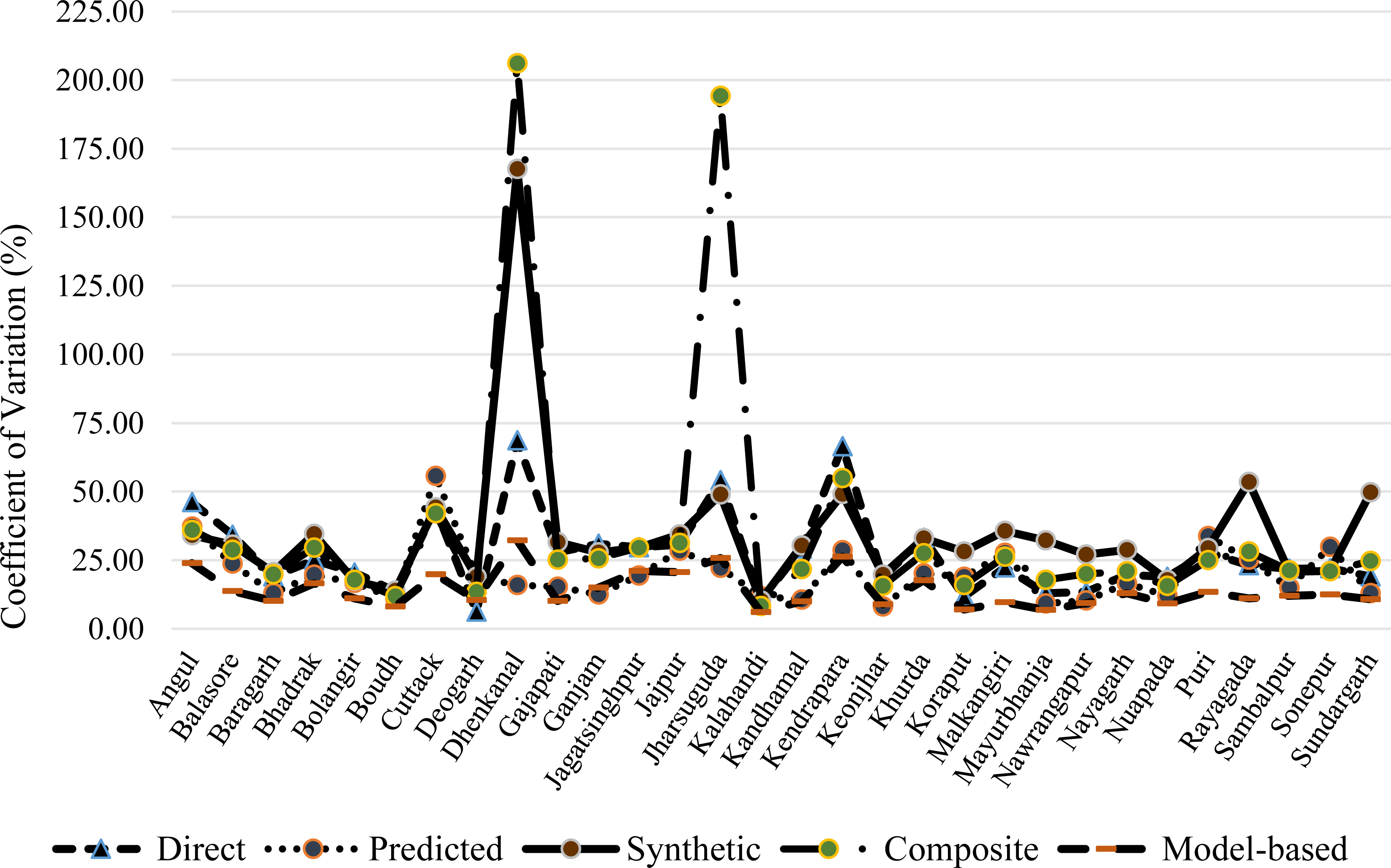

Map 1.

Estimation of poverty of Odisha (model based method).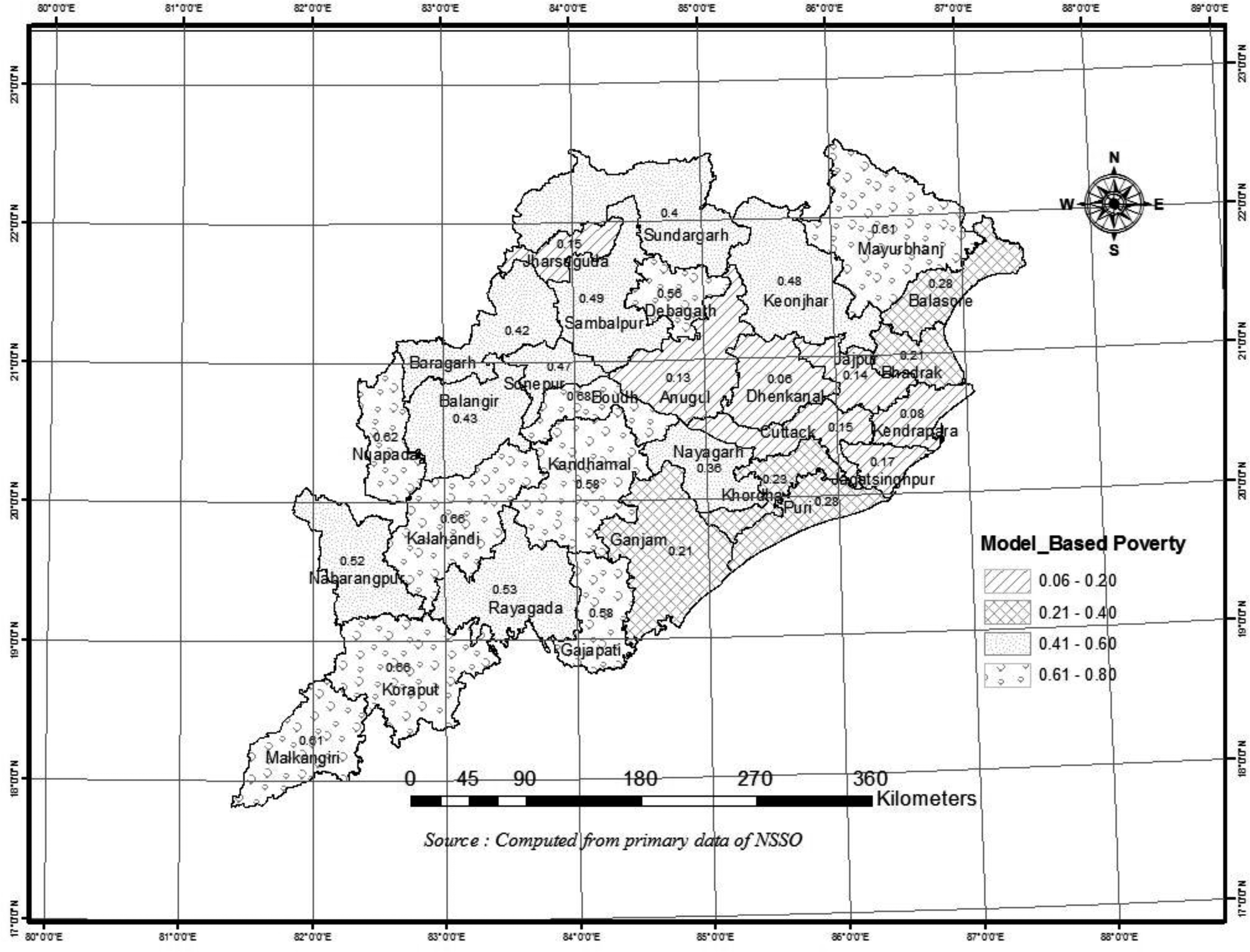

As the model based method is supposed to be reliable method (CV within 30%), the classification of percentage of poverty and poverty mapping has been made based on estimates derived using mixed model method. It is observed that seven districts come under mild, six districts under moderate and seventeen districts under severe category. It implies that more than 50% districts of Odisha are under severe poverty. Particularly, the Southern region of Odisha which are hilly and tribal dominated districts are more vulnerable than the other regions in case of poverty incidence. Only six districts namely Bhadrak, Ganjam, Khordha, Balasore, Puri, and Nayagarh are come under moderate category (20–40%) of poverty.

6. Summary and conclusions

In India the district is an important domain for planning process in the State and therefore, availability of the district level statistics is vital for monitoring the policy and planning. Reliable estimates of poverty at district levels in Odisha are not available except the estimates based on headcount, which are accompanied by large sampling error due to small sample sizes allocated for the districts. This leads to unreliability of the poverty estimates at district levels. In this context the recently developed small area estimation pioneered techniques developed by Rao (2003), Ghosh and Rao (1994), Saei and Chambers (2003), Manteiga et al. (2007) and Chandra et al. (2011) have been applied to capture the district level poverty for Odisha.

The method of estimation of poverty proportion for small areas using reliable small area estimation technique is well developed and practised widely in many countries of the world. But, there is very less known application to the Indian data and no application to the valuable and informative NSSO data for Odisha.

The present analysis using model-based method is found to be more reliable than the direct and indirect methods for computing district level estimates of proportion of poor households in Odisha by using the 68 ${}^{\rm th}$ round NSSO survey rural sector consumer expenditure data and 2011 Population Census. The diagnostic procedures have confirmed that the model-based district level estimates have reasonably good precision. This study produces reliable statistics at micro-level using existing surveys and other already available auxiliary variables and may be seen as a modest attempt in this direction in Odisha. This exercise can be undertaken without conducting micro-level specific survey which may involve a lot of financial burden to the State exchequer and can provide the micro-level estimates for important socio-economic and demographic parameters on regular basis.

Footnotes

Acknowledgments

The authors thank the reviewers for their helpful suggestions. Special thanks go to Dr. Hukum Chandra for his valuable comments and academic discussions which helped the presentation of results to a great extent.

References

Battese

G. E.

Harter

R. M.

, & Fuller

W. A.

(1988). An error component model for prediction of country crop areas using survey and satellite data. Journal of the American Statistical Association, 83, 28-36.

Chandra

Sud

U. C.

, & Salvatri

(2011). Estimation of district level poor households in the State of Uttar Pradesh in India by combining NSSO survey and census data. Journal of the Indian Society of Agricultural Statistics, 65(I), 1-8.

Census of India Volumes (2011). Registrar General, Government of India.

Consumer Expenditure Survey, 2011–12, National Sample Survey Office, Government of India.

Fay

R. E

, & Herriot

R. A.

(1979). Estimates of income for small places: An application of James Steir procedures to census data. J Amer Statist Association, 85, 398-409.

Ghosh

, & Rao

J. N. K.

(1994). Small area estimation and appraisal (with discussion). Statistical Science, 9, 65-93.

Gonzalez

M. E.

(1973). Use and evaluation of synthetic estimators. Proceedings of the Social Statistics Section, American Statistical Association, 33-36.

Holt

Smith

T. M. F.

, & Tomberlin

T. J.

(1979). A model based approach to estimation for small subgroups of a population. Journal of the American Statistical Association, 74, 405-410.

Manteiga

G. W.

Lombardia

M. J.

Molina

Morales

, & Santamaria

(2007). Estimation of the mean squared error of predictors of small area linear parameters under a logistic mixed model. Compute Statistical Data Analysis, 51, 2720-2733.

10.

Prasad

N. G. N.

, & Rao

J. N. K.

(1990). The estimation of the mean squared error of small area estimators. Journal of the American Statistical Association, 85, 163-171.

11.

Rao

J. N. K.

(2003). Small Area Estimation. Wiley Series in Survey Methodology, Jhone Wiley and Sons Inc.

12.

Saei

, & Chambers

(2003). Small area estimation under linear and generalised linear mixed models with time and area effects. Southampton Statistical Sciences Research Institute, University of Southampton, UK, W. P. No. M03/15.

13.

Sisodia

B. V. S.

, & Singh

(2001). Small area estimation – an empirical study. Journal of the Indian Society of Agricultural Statistics, 54(3), 301-316.

14.

Srivastava

A. K.

(2016). Historical perspective and some recent trends in sample survey applications. Statistics and Applications, 14(1-2), 131-143.

District level poverty estimation for rural Odisha (India) using different estimation techniques

Abstract

Keywords

1. Introduction

2. Data

3. Sampling design

Table 1 Distribution of districts-wise rural sample size

5. Methods of estimation of poverty

5.1 Direct method

5.2 Indirect methods

5.2.1 Synthetic estimators

5.2.2 Matching variables in the survey and the census

5.2.3 Selection of covariates

5.3.1 Area level models

Footnotes

Acknowledgments

References

Table 1
Distribution of districts-wise rural sample size