Determination of optimum medical cut points for continuous covariates in lifetime regression models

Abstract

The estimation of optimum cut points for covariates in lifetime regression models is of great interest under a medical view. Usually the choice of covariate cut points is made in an arbitrary way following the clinical expert knowledge. In this paper, it is proposed a simple and practical Bayesian approach which could be used to different lifetime distributions under AFT (accelerated failure time) modeling approach assuming censored or uncensored data to get optimum cut points with larger prognostic effects. For the Bayesian approach, MCMC simulations are used to get estimation for the cut points under a squared error loss (SEL) function. The proposed methodology is illustrated with three medical lifetime data sets.

Keywords

Lifetime data censoring accelerated failure time models cut points Bayesian approach MCMC methods

1. Introduction

Some parametric distributions like the Weibull, log-normal, gamma, generalized gamma distributions or non-parametric methods as the popular Kaplan-Meier (1958) estimates for the survival function and the Wilcoxon and log-rank tests (see, for example, Lee & Wenyuwang, 2003) used in the comparison of two or more treatment groups are usual methods in the analysis of lifetime data for homogeneous populations.

In medical studies, considering survival data, it is also common the presence of concomitant information like gender, age and status of the disease in the diagnostic associated to each patient denoted as covariates, explanatory variables or independent variables. The covariates can be considered as dependent or independent of time. They can be categorical like treatment and ethnicity or be continuous like blood pressure or height. Popular choices of regression models to incorporate the covariates are the proportional hazards model, the additive hazards model, the proportional odds model and the accelerated failure time model (see for example, Collett, 2003; Klein & Moeschberger, 2003; Meeker & Escobar, 1998; Kalbfleisch & Prentice, 2002).

The use of the Cox proportional hazards (Cox, 1972) regression model (or the equivalent in the case of two treatment groups, the log-rank test) is well established as common practice in the statistical analysis of medical data. The great popularity of this model is motivated by being free of a parametric distribution assumption for the survival times.

Usually many of the covariates of interest are continuous. Although these covariates could be modeled as continuous variables, it is common in medical applications to dichotomize continuous covariates to develop prognostic models. In this way, under a statistical approach, dichotomization eliminates the need for the linearity assumption under a regression model, makes data summarization more efficient, and allows for simple interpretation using the impact of a binary covariate on an outcome that it is easier than the interpretation of a regression parameter based on a change of one unit in a continuous covariate. Another great simplification: from the clinical approach, binary covariates give simple risk classification in terms of high versus low, simplify treatment recommendations and simplify the diagnostic criteria (Mazumdar & Glassman, 2000).

In terms of statistical interpretations although all advantages of dichotomization in terms of clinical interpretations, dichotomization could result in the loss of information considering a threshold association rather than a linear relation. In this situation, researchers could not be able to detect possible non-linear relationships (Altman & Royston, 2006; MacCallum et al., 2002). It has been emphasized that dichotomization is appropriate only when a threshold effect value truly exists, that is, if it is possible to assume some binary split of the continuous covariate that creates two relatively distinct but homogeneous groups with respect to a particular outcome (Abdolell et al., 2002).

In general, clinicians point out that the interpretation of continuous covariates could be difficult and they prefer to model these effects as categorical or binary covariates reflecting different prognostic groups of patients based on the measured value of the continuous covariate. In other cases, the covariate may represent the dose of some drug or some other therapeutic agent, and the clinician is interested in identification of a therapeutic threshold.

Even though evaluation of a variable’s prognostic value is best done with the variable in its continuous form and there is a possible loss of information when categorizing a continuous covariate, the need for thresholds for clinical use and treatment decisions justifies the development of appropriate statistical methods for finding optimal cut points (see for example, Lausen et al., 2004; Silva & Klein, 2011; Andrei & Murray, 2007; Lausen & Schumacher, 1996; Abdolell et al., 2002; Altman, 1991, 1998; Hollander & Schumacher, 2001; Hilsenbeck & Clark, 1996; Mazumdar et al., 2003; Altman et al., 1994; Contal & O’Quigley, 1999; Mazumdar & Glassman, 2000; Cumsille et al., 2000; Liquet & Commenges, 2001; Hollander et al., 2004; Ragland, 1992; Magder & Fix, 2003).

Considering a clinical point of view, usually binary covariates could be preferred based on some justifications as follows:

•
A simple risk classification into “high” versus “low”.
•
Criteria for prospective studies.
•
Criteria to make treatment recommendations.
•
Diagnostic criteria for the disease.
•
Estimation of prognosis.
•
To establish an assumed biological threshold.
•
Easiness to obtain association measures easily interpretable as odds ratio or hazard ratio.

When discretizing a continuous covariate and then testing for the covariate effect, a number of techniques can be used. One group of techniques relies on the investigator to provide cut points based on historical data or it uses cut points based on a split into groups at a predetermined percentile of the continuous covariate. Another approach is to let the data decide on the cutpoint and then perform the test of the covariate effect on the two resulting groups. In most cases the continuous covariate in this approach is split into groups based on either the largest value of the likelihood or the largest value of some two-sample test statistic after a search of possible cut points. This selection of the largest likelihood or test statistic leads to an inflated type-I error due to multiple testing, so some correction needs to be applied to obtain the correct type-I error.

Considering medical survival data, the literature presents many different approaches to select a cutpoint based on a data-dependent approach as for example considering a Cox proportional hazards model with a single covariate defined as 1 or 0 depending on the value of the continuous covariate. One of these approaches is based on an adjusted test on the maximum value of the score statistic from the Cox model and convergence to a Brownian bridge under the null hypothesis (Jespersen, 1986). Other approach is based on a modification of the log rank test statistic (Contal & O’Quigley, 1999) showing that the process consisting of the score statistics using cut points at the order statistics of the continuous covariates converges to a Brownian bridge process. Other approaches are introduced in the literature (Lausen & Schumacher, 1992, 1996). Klein and Wu (2004) compare these estimators and extend the Contal and O’Quigley approach to the accelerated failure time model and the Cox model with additional covariates.

A simple alternative for these existing approaches is the use of Bayesian methods especially using computer intensive MCMC (Markov Chain Monte Carlo) methods as the Gibbs sampling algorithm (see for example, Gelfand & Smith, 1990) or the Metropolis-Hastings algorithm (see for example, Chib & Greenberg, 1995) to find optimal cut points for the continuous covariates. In this way, it is possible to obtain in a simple computational way the Bayesian point estimates for the cut points given by Monte Carlo estimates of the posterior means (use of squared error loss function), accurate credible intervals for the cut points and estimates for the regression parameters based on the simulated Gibbs samples. Under a Bayesian approach, the posterior inferences are obtained within a Markov chain Monte Carlo (MCMC) sampling environment using the Open Bugs software (Spiegelhalter et al., 2003).

The paper is organized as follows: in Section 2, it is introduced the general accelerated failure time (AFT) model; in Section 3, it is introduced cut points in AFT models assuming a Weibull distribution for $T$ ; in Section 4, it is introduced some examples with censored and uncensored lifetime data to illustrate the proposed methodology; finally, in Section 5, it is presented some concluding remarks.
2. General accelerated failure time models

In accelerated failure time models (AFT) the effect of the covariates is given by a multiplication of the expected survival time. A general formulation for the AFT hazard for an individual $i$ with $p$ covariates summarized in vector $x_{i}$ is,

$\displaystyle h_{i}(t)=e^{-\eta_{i}}h_{0}\left(\frac{t}{e^{\eta_{i}}}\right)$ (1)

where,

$\displaystyle\eta_{i}=\bm{\beta}^{\prime}\bm{x}_{\bm{i}}=\beta_{1}x_{1i}+\beta% _{2}x_{2i}+\ldots+\beta_{p}x_{pi},$ (2)

$\bm{\beta}^{\prime}=(\beta_{1},\beta_{2},\ldots,\beta_{p})$ is the regression parameter vector, $\bm{x}_{\bm{i}}=(x_{1i},x_{2i},\ldots,x_{pi})$ is the vector of covariates and $h_{0}$ is the hazard function for an individual where $x_{i}=0$ . This $h_{0}$ is also called the baseline hazard.

For AFT models it is common to use the log-linear representation,

$\displaystyle Y=\log(T)=\mu+\bm{\beta^{\prime}x}+\sigma\varepsilon$ (3)

where $\mu$ and $\sigma$ are respectively, intercept and scale parameters, where $\bm{\beta}^{\prime}=(\beta_{1},\beta_{2},\ldots,\beta_{p})$ is the regression parameter vector, $\bm{x}_{\bm{i}}=(x_{1i},x_{2i},\ldots,x_{pi})$ is the vector of covariates and $\varepsilon$ is the error term. The vector $\bm{\beta}$ is the unknown vector of regression coefficients reflecting the effect that each explanatory variable have on the survival time. Positive $\beta_{j}$ means that if covariate $x_{j}$ increases, then the expected survival time increases, and if $\beta_{j}$ is negative, an increasing $x_{j}$ will lead to a decreasing expected survival time.

In applications it is common the use of maximum likelihood approach to get estimation of the unknown parameters in the log-linear regression models. The likelihood function is obtained assuming a distribution of the error. Let us assume $x_{0}=1$ and $\beta_{0}=\mu$ ; also let $f_{\epsilon}(\varepsilon)$ be the probability density function (PDF) of the error term; then the probability density function of the random variable $Y$ is given by,

$\displaystyle f(y)=\sigma^{-1}f_{\epsilon}(\varepsilon)$ (4)

From Eq. (4), the likelihood function in presence of censoring data is given by,

$\displaystyle L(\bm{\beta},\sigma)=\prod\nolimits_{i=1}^{n}{[\sigma^{-1}f_{% \epsilon}\left(\varepsilon_{i}\right)]}^{\delta_{i}}S_{\epsilon}(\varepsilon_{% i})^{1-\delta_{i}}$ (5)

where $S_{\varepsilon}(t)$ denotes the survival function $P(\varepsilon>t)$ , $\varepsilon_{i}=[\log(t_{i})-\beta x_{i}]/\sigma$ and $\delta$ is an censoring indicator variable with $\delta_{i}=1$ if we observe a complete lifetime and $\delta_{i}=0$ if we have a censoring time.

Maximum likelihood estimates for $\mathrm{\beta}$ and $\mathrm{\sigma}$ denoted by $\hat{\beta}$ and $\hat{\sigma}\mathrm{}$ are obtained maximizing the likelihood Eq. (5). Confidence intervals and hypotheses tests of interest are usually obtained from the asymptotical multivariate normal distribution for the maximum likelihood estimates $(\hat{\beta},\hat{\sigma})\sim N\{(\beta,\sigma);I_{0}^{-1}\}$ , where $I_{0}$ is the observed Fisher information matrix (see for example, Lawless, 1982).

A popular regression model derived from Eq. (3) is given by the Weibull regression model where the term $\mathrm{\varepsilon}$ is a random quantity with an extreme value distribution (see for example, Nelson, 2004 or Lawless, 1982) also defined as an extreme value distribution of type I (minimum) or Gumbel distribution (see, Gumbel, 1954) with a probability density function given by,

$\displaystyle f_{\epsilon}(\varepsilon)=\exp\{\varepsilon-\exp(\varepsilon)\},% -\infty<\varepsilon<\infty$ (6)

The parameter $\mathrm{\sigma}$ is related to the shape parameter of the Weibull distribution by the relationship $\mathrm{\sigma=1/\alpha}$ , with Weibull density given by,

$\displaystyle f(t_{i})=\frac{\alpha t_{i}^{\alpha-1}}{\lambda^{\alpha}}\exp% \left\{-\left(\frac{t_{i}}{\lambda}\right)^{\alpha}\right\}$ (7)

The survival function and hazard functions of the Weibull distribution with density Eq. (7) are given, respectively, by,

$\displaystyle S(t)=\exp\left\{-\left(\frac{t}{\lambda}\right)^{\alpha}\right\}$

and

$\displaystyle\lambda(t)=\frac{{\gamma t}^{\gamma-1}}{\alpha^{\gamma}}$ (8)

The hazard function $\mathrm{\lambda(t)}$ of the Weibull distribution given in Eq. (8) is increasing if $\mathrm{\alpha>1}$ ; decreasing if $\mathrm{\alpha<1}$ and constant (exponential distribution) if $\mathrm{\alpha=1}$ . The mean and variance are given, respectively, by,

$\displaystyle E(T)=\lambda\Gamma\left[1+\left(\frac{1}{\alpha}\right)\right]$

and

$\displaystyle\textit{Var}(T)=\lambda^{2}\left\{\Gamma\left[1+\left(\frac{2}{% \alpha}\right)\right]-\Gamma^{2}\left[1+\left(\frac{1}{\alpha}\right)\right]\right\}$ (9)

Also note that from model Eq. (3), the scale parameter $\mathrm{\lambda}$ defined in Eq. (7) is related with the covariates vector from the relationship,

$\displaystyle\lambda_{i}=\exp(\beta_{0}+\beta_{1}x_{1i}+\ldots+\beta_{p}x_{pi})$ (10)

that is, the regression model defined by Eq. (3) defines a regression model in the scale parameter (see for example, Lawless, 1982) assuming the same shape parameter.

The log-linear regression model Eq. (3) can be extended to other distributions for $\mathrm{\varepsilon}$ or $\mathrm{T}$ . Some usual choices for $\mathrm{T}$ : log-normal, gamma and log-logistic distributions. In this case, we have normal, log-gamma and logistic distributions for the error $\mathrm{\varepsilon}$ .

3. Cut points in AFT models assuming a Weibull distribution for T

Let us assume a Weibull distribution for the lifetimes $T$ and the AFT regression model given by Eq. (3) assuming that all covariates are continuous and we are interested to find the best cut points for the continuous covariates $X_{1},X_{2},\ldots,X_{p}$ . Suppose that the $i^{\rm th}$ subject has the response variable $Y_{i}=\log(T_{i})$ , $i=1,2,\ldots,n$ with vector of covariates $X_{i}=(X_{1i},X_{2i},\ldots,X_{pi})$ . Thus, there are $p$ indicator variables, defined by, $I_{[0,\tau_{l}]}(x_{li})=1$ if $x_{li}\leqslant\zeta_{l}$ and $I_{[0,\tau_{l}]}(x_{li})=0$ if $x_{li}>\zeta_{l}$ , $l=1,2,\ldots,p$ ; $i=1,2,\ldots,n$ .

In this way, it is defined the following regression model:

$\displaystyle y_{i}=\log(t_{i})=\beta_{0}+\beta_{1}I_{[0,\mathbf{\tau}_{1}]}(x% _{1i})+\ldots+\beta_{p}I_{[0,\mathbf{\tau}_{p}]}(x_{pi})+\sigma\varepsilon_{i}$ (11)

where $X_{li}\in[0,T_{l}]$ , $l=1,2,\ldots,p$ .

For a Bayesian analysis, it i assumed that the parameters $\beta_{1}$ , $\sigma$ and the cutpoints $\zeta_{l}$ , $l=1,2,\ldots,p$ have the following prior distributions:

$\displaystyle\beta_{l}\sim N(a_{l},b_{l}^{2})$ $\displaystyle\sigma\sim G(c,d)$ (12) $\displaystyle{\zeta}_{l}\sim U(p_{1l},p_{2l})$

where $N(a,b^{2})$ denotes a normal distribution with mean equals to a and variance equals to $b^{2}$ ; $G(c,d)$ denotes a gamma distribution with mean equals to $\frac{c}{d}$ and $U(a,b)$ denotes a continuous uniform distribution. The hyperparameters $a_{l},b_{l}^{2},c,d{,p}_{1l}\text{ and }p_{2l}$ are assumed known. Further it is assumed prior independence among the parameters, that is, the joint prior distribution for the vector of parameters $\theta=(\beta,\sigma,\zeta)$ , $\beta=(\beta_{0},\beta_{1},\ldots,\beta_{p})$ and $\zeta=(\zeta_{1},\ldots,{\zeta}_{p})$ is the product of the prior distributions given in Eq. (3).

Combining the joint prior distribution for $\mathrm{\theta}$ with the likelihood function $\mathrm{L(\theta)}$ given in Eq. (5), the posterior distribution for $\mathrm{\theta}$ is determined from the Bayes formula (see for example, Box & Tiao, 1973), that is,

$\displaystyle\pi(\theta|y,x)\propto\prod\nolimits_{i=1}^{n}{[\sigma^{-1}\exp\{% \varepsilon_{i}-\exp(\varepsilon_{i})\}]}^{\delta_{i}}{[\exp\{-\exp(% \varepsilon_{i})\}]}^{{1-\delta}_{i}}.\prod\nolimits_{l=1}^{p}\exp\{-{(\beta_{% l}-a_{l})}^{2}\}.\sigma^{c-1}e^{-b\sigma}.$

Or,

$\displaystyle\pi(\theta|y,x)\propto\sigma^{-n}\exp\left\{\sum\nolimits_{i=1}^{% n}\delta_{i}\varepsilon_{i}\right\}\left[\prod\nolimits_{i=1}^{n}\exp(-e^{% \varepsilon_{i}})\right].\prod\nolimits_{l=1}^{p}\exp\{-{(\beta_{l}-a_{l})}^{2% }\}.\sigma^{c-1}e^{-b\sigma},$ (13)

where, $\varepsilon_{i}=[y_{i}-\beta_{0}-\beta_{1}I_{[0,\mathbf{\tau}_{1}]}(x_{1i})-% \ldots-\beta_{p}I_{[0,\mathbf{\tau}_{p}]}(x_{pi})]/\sigma,i=1,\ldots,n,-\infty% <\beta_{0}<\infty,-\infty<\beta_{l}<\infty,\sigma>0\text{ and }p_{1l}<{\zeta}_% {l}<p_{1l}$ .

Samples of the joint posterior distribution for $\mathrm{\beta}_{\mathrm{1}}$ , $\mathrm{\sigma}$ and ${\mathrm{\zeta}}_{\mathrm{l}}$ are obtained using MCMC methods as the popular Gibbs sampling algorithm (see for example, Gelfand & Smith, 1990). Notice that the full conditional posterior distributions needed for the Gibbs sampling algorithm are given by,

$\displaystyle\pi(\beta_{0}|\beta(0),\sigma,\zeta,y,x)\propto\exp\left\{-(\beta% _{0}/\sigma)\sum\nolimits_{i=1}^{n}\delta_{i}\right\}\left[\prod\nolimits_{i=1% }^{n}\exp(-e^{\varepsilon_{i}})\right]\exp{(\beta_{0}-a_{0})}^{2}$ $\displaystyle\pi(\beta_{l}|\beta(l),\sigma,\zeta,y,x)\propto\exp\left\{-{(% \beta}_{l}/\sigma)\sum\nolimits_{i=1}^{n}\delta_{i}\beta_{l}I_{[0,\mathbf{\tau% }_{l}]}(x_{li})\right\}\left[\prod\nolimits_{i=1}^{n}\exp(-e^{\varepsilon_{i}}% )\right]\exp{(\beta_{l}-a_{l})}^{2}$ (14) $\displaystyle\pi(\sigma|\beta,\zeta,y,x)\propto\exp\left\{\sum\nolimits_{i=1}^% {n}\delta_{i}\varepsilon_{i}\right\}\left[\prod\nolimits_{i=1}^{n}\exp(-e^{% \varepsilon_{i}})\right]\sigma^{c-n-1}e^{-b\sigma},$

and

$\displaystyle\pi(\zeta_{l}|\zeta(l),\sigma,\beta,y,x)\propto\exp\left\{\sum% \nolimits_{i=1}^{n}\delta_{i}\varepsilon_{i}\right\}\left[\prod\nolimits_{i=1}% ^{n}\exp(-e^{\varepsilon_{i}})\right]$

where, $l=1,2,\ldots,p$ and do not present known form of probability distribution functions ( $\theta(l)$ denotes all components of the vector $\theta$ , except the component $\theta_{l}$ ). In this way, it is used the Metropolis-Hastings algorithm (see for example, Chib & Greenberg, 1995), to generate samples from the joint posterior distribution of interest.

Bayes estimates for the regression parameters $\beta_{0}$ , $\beta_{l}$ , $\sigma$ and the cutpoints ${\zeta}_{l}$ , $l=1,2,\ldots,p$ are obtained by Monte Carlo estimates for the posterior means (Bayes estimates assuming a SEL function) $E(\beta_{0}|y,x),E(\beta_{l}|y,x)$ , $E(\sigma|y,x)$ and $E(\zeta_{l}|y,x)$ based on the simulated Gibbs samples.

In the same way it is also possible to assume other regression lifetime models as in special case, a log-normal regression model in Eq. (3).

4. Applications

In this section, it is considered different applications of the proposed methodology assuming uncensored and censored medical survival times. For this purpose, three data sets are considered. In each application it was assumed a Bayesian analysis using the Open Bugs software (Spiegelhalter et al., 2003) with a burn-in sample of 11,000 samples deleted to eliminate the effect of the initial values in the iterative algorithm and 100,000 additional samples from where it was considered every 100 ${}^{\rm th}$ sample which gives a total of 1,000 Gibbs samples to be used to get the Monte Carlo estimates of the posterior summaries of interest.

Figure 1.

TTT plot based on the (a) Krall data set, (b) Greene and Byar data set and (c) German breast cancer data set.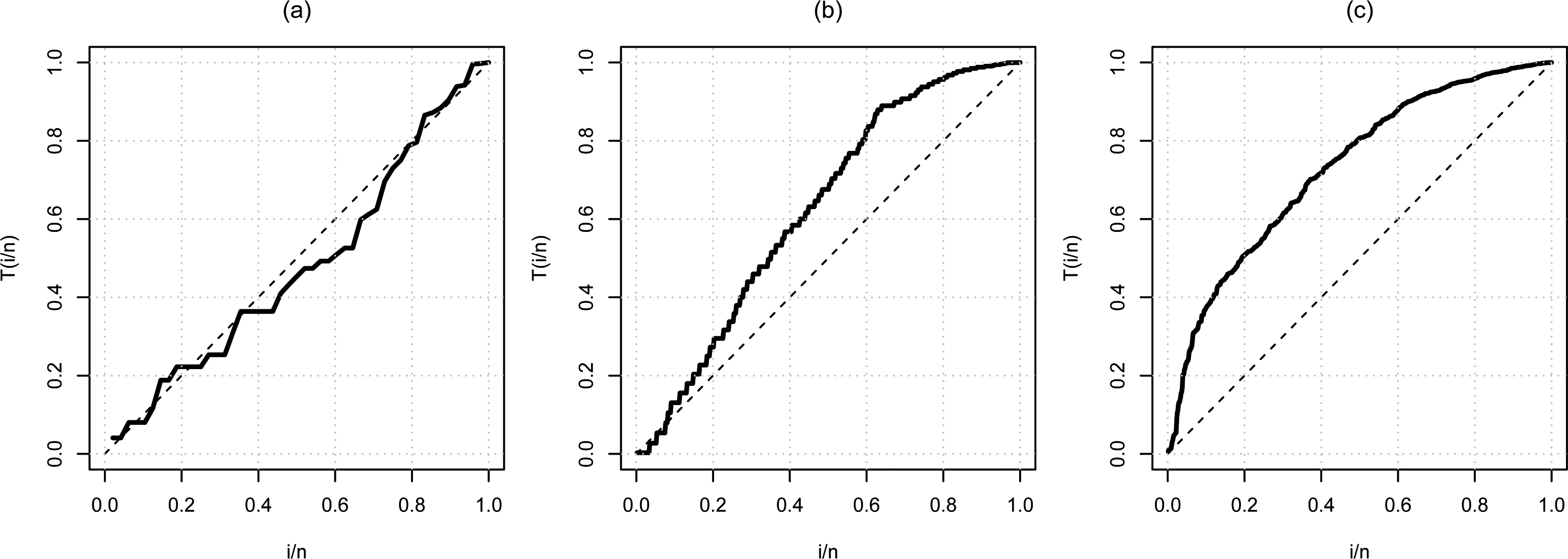

Before doing a modeling, a Total Time on Test (TTT) plot showed that the three data sets do not have constant risk function, one with decreasing risk function and the other two with increasing risk function (Fig. 1), suggesting that the Weibull distribution may be appropriate. The TTT concept was introduced by Barlow et al. (1972).

Convergence of the Gibbs sampling algorithm was observed from trace plots of the simulated Markov Chains (Fig. 9).

4.1 An application with a multiple myeloma uncensored data

The uncensored data set is part from a more extensive data introduced by Krall et al. (1975) (here we only consider the uncensored data). The problem is to relate survival times for multiple myeloma patients to a number of prognostic variables. The survival times (given in months) consists of 48 observations and include measurements on each patient for five covariates: $X_{1}$ : logarithm of a blood urea nitrogen (BUN) measurement at diagnosis; $X_{2}$ : Hemoglobin (Hb) measurement at diagnosis; $X_{3}$ : Age at diagnosis; $X_{4}$ : Gender: 0, male; 1, female; $X_{5}$ : Serum calcium measurement at diagnosis.

For the statistical analysis of the data set, it is assumed a Weibull regression model with density Eq. (7) and regression model Eq. (10) for the scale parameter $\mathrm{\lambda}$ not considering the presence of cutpoints, given by,

$\displaystyle\lambda_{i}=\exp(\beta_{0}+\beta_{1}x_{1i}+\ldots+\beta_{k}x_{ki})$ (15)

for $i=1,2,\ldots,48$ and $k=$ 5. Maximum likelihood estimation method is used to obtain the classical inferences for the model. In Table 2 (a), it is presented the maximum likelihood estimates (MLE) for the parameters of the model.

From the results of Table 2 (a), it is concluded that only the predictor BUN associated with covariate logarithm of a blood urea nitrogen has significative effect on the lifetimes for the patients with multiple myeloma (significative at 5%, since $p$ -value $<$ 0.05).

A visual form to verify the possible existence of cut-off points is from risk functions. The risk ratios of continuous covariates are presented in Fig. 2. Each estimate is presented with a 95% confidence interval, intervals below the dotted line suggest greater risks while the above suggest minor risks. In the chart (a) BUN values above 1.4 present higher risks and in graph (c) in the age ranging between 50 and 70 years there seems to be a risk change.

For a Bayesian analysis of the Weibull regression model Eq. (15) in presence of cut points for the continuous covariates, it is assumed a Weibull distribution in another parametrization with density (parametrization given in the Open Bugs software),

$\displaystyle f(t_{i})=\alpha\gamma t_{i}^{\alpha-1}\exp\{-\gamma t_{i}^{% \alpha}\}$ (16)

and regression model for the scale parameter $\mathrm{\gamma}$ , given by

$\displaystyle\gamma_{i}=\exp[\eta_{0}+\eta_{1}I_{[0,\tau_{1}]}(x_{1i})+\eta_{2% }I_{[0,\tau_{2}]}(x_{2i})+\eta_{3}I_{[0,\tau_{3}]}(x_{3i})+\eta_{4}x_{4i}+\eta% _{5}I_{[0,\tau_{4}]}(x_{5i})]$ (17)

Table 1

Descriptive statistics for the continuous covariate

Data set	Variable	Mean	Minimum	Maximum
Krall data set	BUN	1.39	0.78	2.24
	Hb	9.91	5.00	14.60
	Age	59.25	38.00	81.00
	Serum calcium	10.23	8.00	18.00
Greene and Byar data set	Age	71.57	48.00	89.00
	Weight index	98.95	69.00	152.00
	Systolic	14.36	8.00	30.00
	Diastolic	8.15	4.00	18.00
	Serum hemog	l13.42	5.90	18.20
	Sz	14.40	0.00	69.00
	Sg	10.30	5.00	15.00
	Ap	12.49	0.10	999.88
German breast cancer data set	age	53.05	21	80
	size	29.33	3	120
	nodes	5.01	1	51
	prrecp	110.00	0	2380
	estrrecp	96.25	0	1144

Figure 2.

Risk functions of covariates, (a) logarithm of a blood urea nitrogen (BUN); (b) Hemoglobin (Hb); (c) Age; (d) Serum calcium.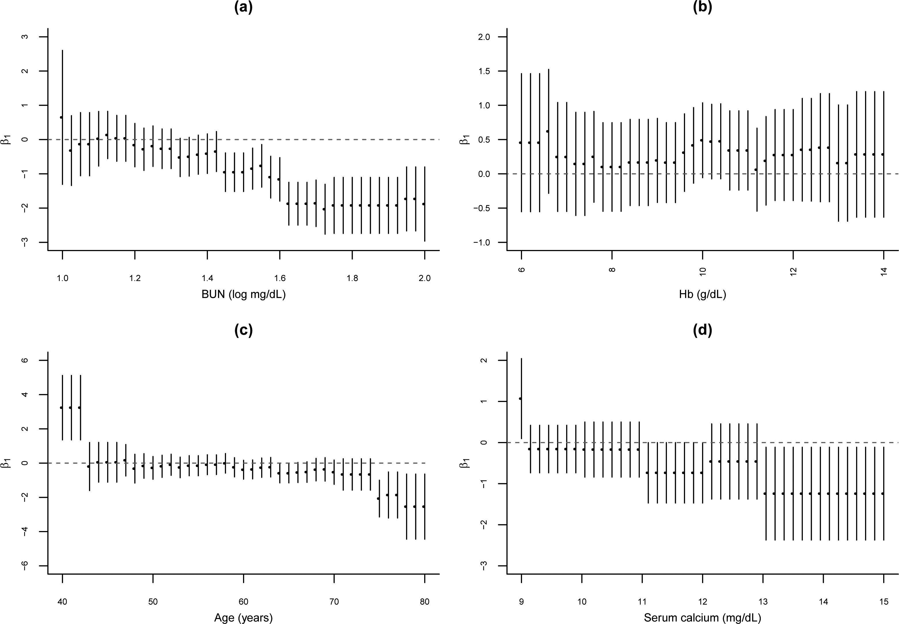

Observe that the covariate $X_{4}$ (gender: 0, male; 1, female) is a binary variable and do not requires the search a cutpoint. In this way there are four cutpoints associated to each continuous covariate $X_{1}$ (logarithm of a blood urea nitrogen measurement at diagnosis), $X_{2}$ (hemoglobin measurement at diagnosis), $X_{3}$ (age at diagnosis) and $X_{5}$ (serum calcium measurement at diagnosis) given respectively by $\zeta_{1}$ , $\zeta_{2}$ , $\zeta_{3}$ and $\zeta_{4}$ . For a Bayesian analysis, it is assumed the following prior distributions for each parameter: $\alpha\sim G(1,1)$ , $\eta_{0}\sim N(1,10)$ , $\eta_{l}\sim N(0,1)$ for $l=1,2,3,4,5$ ; $\zeta_{1}\sim U(1.3,1.7)$ , $\zeta_{2}\sim U(5,14.6)$ , $\zeta_{3}\sim U(45,70)$ and $\zeta_{4}\sim U(8,18)$ . Further it is assumed independence among the parameters. Observe that it is used the information of Table 1 and Fig. 2 to choose the intervals in the uniform priors for the four cut points (use of empirical Bayesian methods; see for example, Carlin & Louis, 1996). Further it is assumed independence among the parameters.

Table 2

MLE estimates for the parameters of the Weibull regression model (Krall data set)

	(a) Continuos covariates				(b) Dichotomized covariates
Predictor	Coefficient	$p$ -value	95% normal CI		Coefficient	$p$ -value	95% normal CI
			Lower limit	Upper limit			Lower limit	Upper limit
Intercept	6.00	0.00	2.96	9.05	3.62	$<$ 0.001	3.08	4.15
BUN	$-$ 1.58	0.01	$-$ 2.70	$-$ 0.46	$-$ 1.89	$<$ 0.001	$-$ 2.49	$-$ 1.30
Hb	0.05	0.40	$-$ 0.06	0.16	0.17	0.49	$-$ 0.31	0.64
Age	$-$ 0.003	0.87	$-$ 0.03	0.03	$-$ 0.38	0.11	$-$ 0.84	0.08
Gender	$-$ 0.01	0.97	$-$ 0.58	0.56	$-$ 0.07	0.78	$-$ 0.54	0.41
Serum calcium	$-$ 0.10	0.29	$-$ 0.28	0.08	$-$ 1.46	$<$ 0.001	$-$ 2.43	$-$ 0.49
Shape	1.08	0.45			1.32		1.06	1.65

Figure 3.

Histograms for the simulated Gibbs samples of the cut points (Weibull regression model – Krall data set).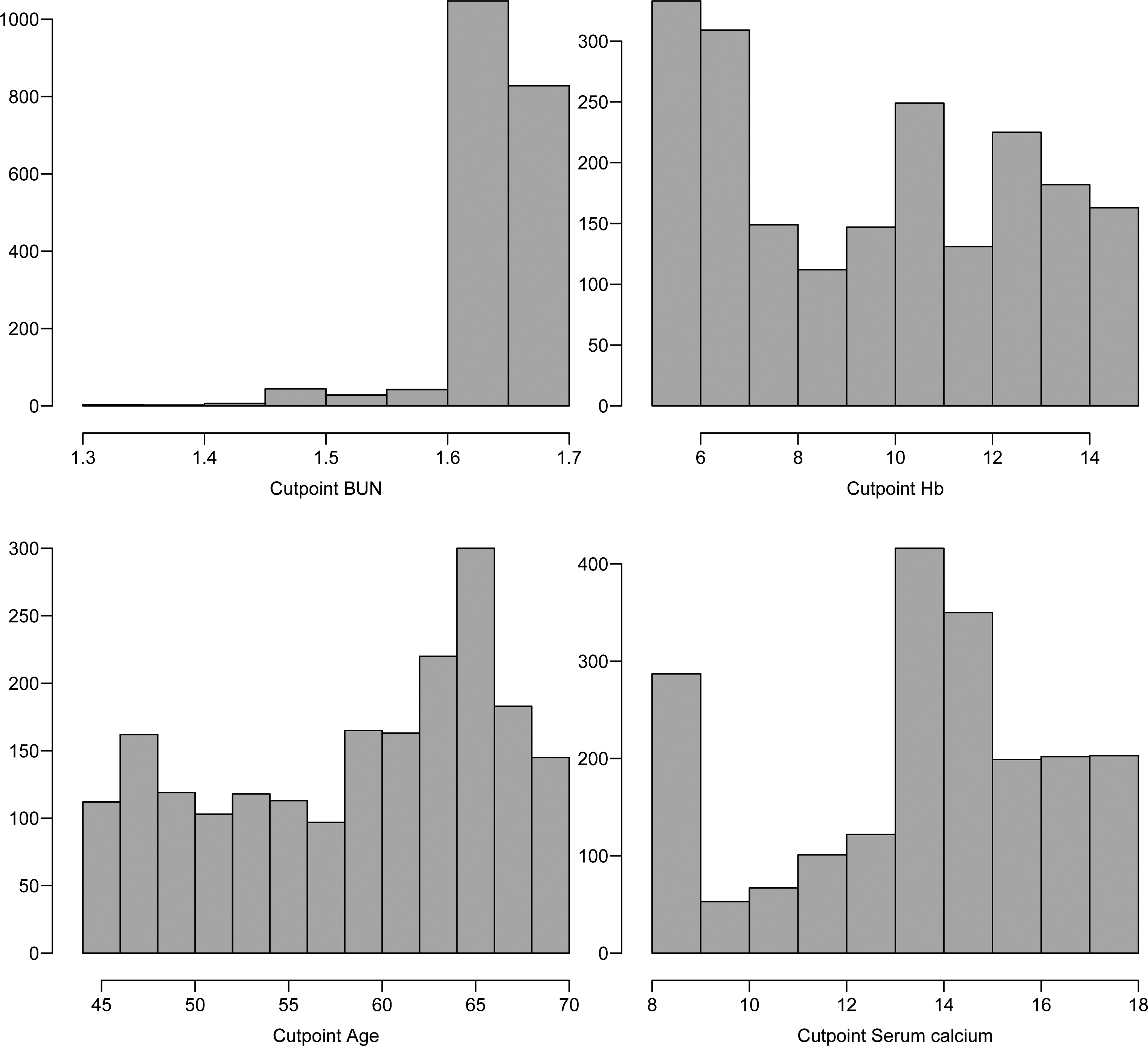

In Table 3, it is presented the posterior summaries of interest (Monte Carlo estimates for the posterior mean, posterior median, posterior standard deviation and 95% credible intervals for each parameter). From the results of Table 3, it is concluded that only the predictor BUN associated with covariate logarithm of a blood urea nitrogen has significative effect on the lifetimes (95% credibility intervals not including the value zero) for patients with multiple myeloma. The cut points for the continuous covariates are respectively estimated by 1.688 (blood urea), 9.484 (hemoglobin), 62.15 (age) and 13.72 (serum calcium).

In Fig. 3, it is presented the histograms of the simulated Gibbs samples for the cut points assuming a Weibull regression model.

From the graphs of Fig. 3, it is observed that the cut point 1 ( $\zeta_{1}$ ) has very accurate Bayesian inference. In fact, this cut point is associated to the covariate BUN (logarithm of a blood urea nitrogen measurement at diagnosis) that has a significative effect on the lifetimes. All other three covariates Hb (hemoglobin measurement at diagnosis), Age (age at diagnosis) and Serum calcium (serum calcium measurement at diagnosis) which do not have significative effects on the response (lifetimes) have correspondent cutpoints very non-informative as observed in the histograms of the cutpoints ( $\zeta_{2}$ , $\zeta_{3}$ and $\zeta_{4}$ ) presented in Fig. 3. That is, the proposed approach has good performance to estimate the cutpoints of the continuous covariates.

Based on the cut points given in Table 3, Kaplan-Meier survival curves are estimated for each dichotomized covariate.

From the graphs of Fig. 4, it is possible to observe that the covariate logarithm of a blood urea nitrogen measurement at diagnosis and serum calcium measurement at diagnosis have distinct groups at survival times.

Table 3

Posterior summaries for the Weibull regression model considering the presence of cut points (Krall data set)

	Mean	Standard deviation	Median	95% Credibility interval
				Lower limit	Upper limit
Intercept	$-$ 3.60	0.81	$-$ 3.66	$-$ 5.00	$-$ 1.70
BUN	1.65	0.51	1.68	0.57	2.62
Hb	$-$ 0.31	0.51	$-$ 0.31	$-$ 1.36	0.76
Age	0.21	0.41	0.24	$-$ 0.67	0.96
Gender	$-$ 0.16	0.31	$-$ 0.15	$-$ 0.80	0.41
Serum calcium	0.52	0.89	0.56	$-$ 1.33	2.15
$\alpha$	1.15	0.13	1.15	0.91	1.44
$\zeta_{1}$ (BUN)	1.64	0.04	1.64	1.50	1.70
$\zeta_{2}$ (Hb)	9.51	3.04	9.84	5.19	14.42
$\zeta_{3}$ (Age)	58.54	7.43	60.10	45.47	69.47
$\zeta_{4}$ (Serum calcium)	13.50	2.80	13.90	8.16	17.79

Figure 4.

Plots of Kaplan-Meier estimates for dichotomized covariates, (a) logarithm of a blood urea nitrogen (BUN); (b) Hemoglobin (Hb); (c) Age; (d) Serum calcium.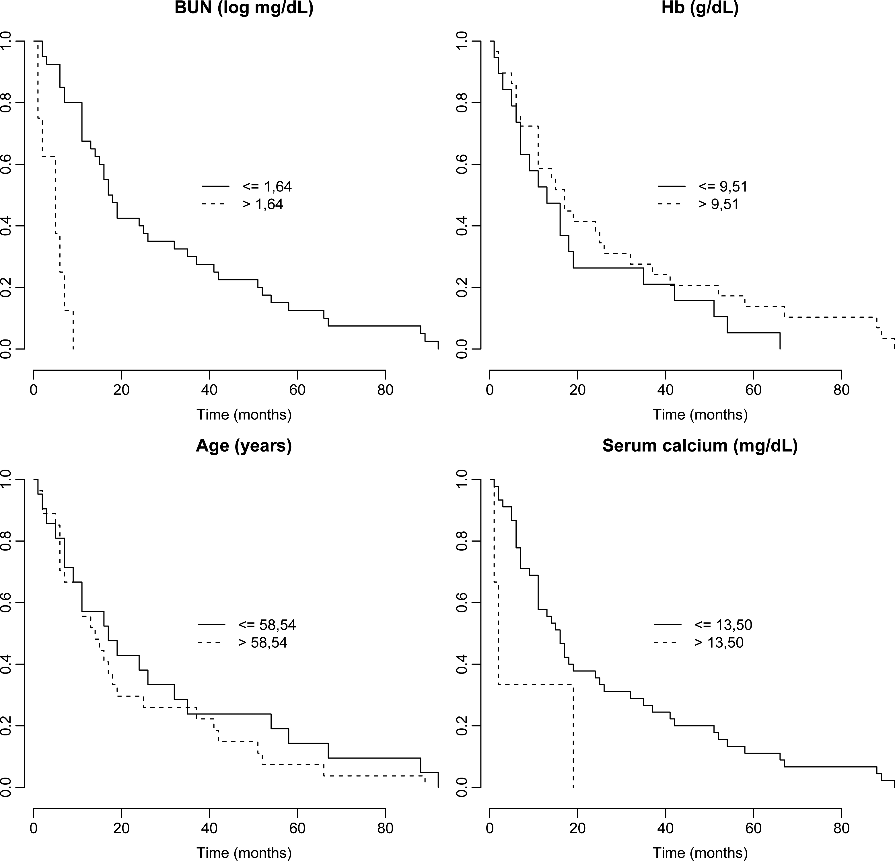

Assuming the dichotomized covariates, in Table 3 it is presented the maximum likelihood estimates (MLE) for the parameters of the model in Eq. (15). From the results of Table 2 (b), it is concluded that the predictor BUN has significative effect and Serum calcium also has a significative effect on the lifetimes for the patients with multiple myeloma (significative at 5%, since $p$ -value $<$ 0.05).

Table 4

MLE estimates for the parameters of the Weibull regression model (Greene and Byar data set)

	(a) Continuos covariates				(b) Dichotomized covariates
Variable	Coefficient	$p$ -value	95% normal CI		Coefficient	$p$ -value	95% normal CI
			Lower limit	Upper limit			Lower limit	Upper limit
Intercept	3.72	0.0045	1.16	6.28	3.97	0.0000	2.08	5.86
Stage 4	$-$ 0.42	0.0708	$-$ 0.88	0.04	$-$ 0.90	0.0000	$-$ 1.30	$-$ 0.51
Age	0.02	0.0910	0.00	0.04	0.18	0.7640	$-$ 1.00	1.37
Weight index	0.00	0.8000	$-$ 0.01	0.01	0.16	0.4960	$-$ 0.30	0.62
Carddisease 1	$-$ 0.08	0.6170	$-$ 0.40	0.23	$-$ 0.02	0.8950	$-$ 0.34	0.30
Systolic	0.02	0.6250	$-$ 0.06	0.10	0.03	0.9400	$-$ 0.73	0.79
Diastolic	0.05	0.5030	$-$ 0.09	0.18	0.51	0.0551	$-$ 0.01	1.03
Serum hemogl	0.10	0.0175	0.02	0.18	0.55	0.0184	0.09	1.01
Sz	$-$ 0.03	0.0000	$-$ 0.04	$-$ 0.02	$-$ 1.03	0.0000	$-$ 1.39	$-$ 0.68
Sg	$-$ 0.16	0.0017	$-$ 0.26	$-$ 0.06	0.55	0.5100	$-$ 1.09	2.20
Ap	0.00	0.5720	0.00	0.00	$-$ 0.02	0.9830	$-$ 1.69	1.65
Bm 1	$-$ 0.39	0.0494	$-$ 0.77	0.00	$-$ 0.62	0.0011	$-$ 1.00	$-$ 0.25
Rx 1	$-$ 0.07	0.7290	$-$ 0.44	0.31	$-$ 0.01	0.9790	$-$ 0.38	0.37
Rx 2	0.69	0.0027	0.24	1.14	0.76	0.0012	0.30	1.22
Rx 3	0.58	0.0088	0.15	1.01	0.63	0.0047	0.19	1.06
Shape	0.81	0.0062			$-$ 0.19	0.0123

Table 5

Posterior summaries for the Weibull regression model in the presence of cut points (Greene and Byar data set)

	Mean	Standard deviation	Median	95% credibility interval
				Lower limit	Upper limit
Intercept	$-$ 5.07	1.28	$-$ 4.87	$-$ 6.83	$-$ 3.60
Stage	0.84	0.21	0.90	0.42	1.13
Age	$-$ 0.49	0.71	$-$ 0.37	$-$ 2.06	0.82
Weight index	$-$ 0.38	0.41	$-$ 0.32	$-$ 1.66	0.22
Carddisease	0.00	0.18	$-$ 0.01	$-$ 0.40	0.37
Systolic	$-$ 0.67	0.51	$-$ 0.66	$-$ 1.60	0.26
Diastolic	$-$ 0.63	0.87	$-$ 0.61	$-$ 2.44	0.80
Serum hemogl	$-$ 1.18	0.67	$-$ 1.18	$-$ 2.36	$-$ 0.16
Sz	1.29	0.29	1.32	0.88	1.65
Sg	$-$ 1.30	0.75	$-$ 1.46	$-$ 2.66	$-$ 0.09
Ap	$-$ 0.34	0.72	$-$ 0.31	$-$ 1.86	0.91
Bm	0.60	0.24	0.62	0.19	1.10
Rx	$-$ 0.14	0.05	$-$ 0.14	$-$ 0.26	$-$ 0.03
$\alpha$	1.12	0.10	1.13	0.95	1.30
$\zeta 1$ age	81.80	4.26	82.48	73.85	88.60
$\zeta 2$ weight index	81.91	6.48	81.89	69.30	92.98
$\zeta 3$ systolic	10.41	2.83	9.57	8.05	21.07
$\zeta 4$ diastolic	9.50	3.37	10.23	4.10	16.36
$\zeta 5$ serum hemogl	10.42	2.48	9.27	7.40	15.34
$\zeta 6$ sz	27.82	1.92	26.96	26.04	32.70
$\zeta 7$ sg	5.76	0.72	5.58	5.03	7.81
$\zeta 8$ ap	408.20	22.49	409.00	367.10	443.90

Figure 5.

Histograms for the simulated Gibbs samples of the cut points (Weibull regression model – Greene and Byar data set).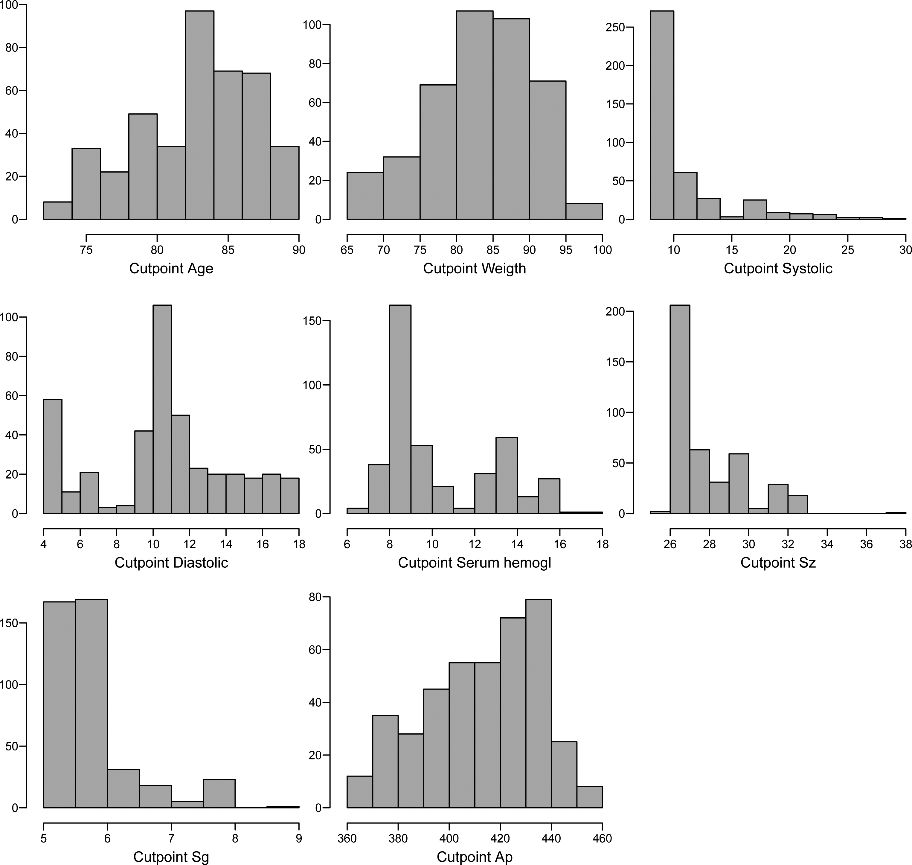

4.2 An application with a prostate cancer censored data set

As a second application, let us consider the Greene and Byar (1980) prostate cancer data in presence of censored data, available in the Andrews and Herzberg (1985). The original data set consists of 502 observations and 18 variables. In our study it was deleted some missing data (it was considered a total of $n=$ 483 observations) considering the following variables: the responses given by the survival times denoted by time (months of follow-up) and the covariates:

1.
Stage: Stage (3 or 4),
2.
Age: (in years),
3.
Weightindex: (wt (kg) $-$ ht (cm) $+$ 200),
4.
Carddisease: Carddisease (0 or 1),
5.
Systolic: (systolic blood pressure/10),
6.
Diastolic: (diastolic blood pressure/10),
7.
Hemogl: Serum hemogl (mg/dL),
8.
sz: (size of primary tumor in cm ${}^{2}$ ),
9.
sg: (combined index of stage and hist. grade) (5–15),
10.
ap: (serum prostatic acid phosphatase),
11.
bm: (bone metastases) (0 or 1),
12.
rx: (placebo $=$ 0, 0.2 mg estrogen, 1.0 mg estrogen, 5.0 mg estrogen).

The censoring variable is given by status (1 $=$ dead from prostatic cause and 0 $=$ alive or death from other causes). The dataset has 125 uncensored lifetimes (death from prostate cancer) and 358 right censored values (alive or death from other causes).

Similarly to the first example, it is assumed a Weibull regression (see Eq. (15)) with $i=1,\ldots,483$ and $k=$ 12 where, $X_{1}=$ stage, $X_{2}=$ age, $X_{3}=$ weight index, $X_{4}=$ carddisease, $X_{5}$ $=$ systolic, $X_{6}=$ systolic, $X_{7}=$ serum hemogl, $X_{8}=$ sz, $X_{9}=$ sg, $X_{10}=$ ap, $X_{11}=$ bm, $X_{12}=$ rx. Maximum likelihood estimation method (MLE) was used to obtain the estimates for the parameters of the model given in Table 4 (a).

From the results of Table 4 (a), it is concluded that the covariates with significative effects on the lifetimes for patients with prostate cancer are:

•
Significative at 5% ( $p$ -value $<$ 0.05): Serum hemogl, sz, sg, bm, rx,
•
Significative at 10% ( $p$ -value $<$ 0.10): Stage, age.

Table 6
MLE estimates for the parameters of the Weibull regression model (German breast cancer study data set)

(a) Continuos covariates (b) Dichotomized covariates

Predictor Coefficient $p$ -value 95% normal CI Coefficient $p$ -value 95% normal CI

Lower limit Upper limit Lower limit Upper limit

Intercept 8.93 0.0000 8.11 9.74 7.53 0.0000 6.27 8.78

Age 0.00 0.5730 $-$ 0.02 0.01 0.95 0.1090 $-$ 0.21 2.11

Menopause $-$ 0.06 0.7000 $-$ 0.35 0.23 $-$ 0.14 0.1540 $-$ 0.33 0.05

Hormone 0.17 0.0849 $-$ 0.02 0.36 0.19 0.0495 0.00 0.38

Size $-$ 0.01 0.0054 $-$ 0.01 0.00 $-$ 0.52 0.0081 $-$ 0.90 $-$ 0.14

Grade 2 $-$ 0.46 0.0701 $-$ 0.95 0.04 $-$ 0.28 0.2600 $-$ 0.78 0.21

Grade 3 $-$ 0.67 0.0105 $-$ 1.19 $-$ 0.16 $-$ 0.48 0.0696 $-$ 0.99 0.04

Nodes $-$ 0.03 0.0000 $-$ 0.04 $-$ 0.02 $-$ 0.63 0.0000 $-$ 0.82 $-$ 0.43

Prog_recp 0.00 0.0000 0.00 0.00 0.70 0.0000 0.44 0.96

Estrg_recp 0.00 0.6840 0.00 0.00 0.11 0.3280 $-$ 0.11 0.34

Shape $-$ 0.53 0.0000 $-$ 0.54 0.0000

Figure 6.
Plots of Kaplan-Meier estimates for dichotomized covariates, (a) Age; (b) Weight; (c) Systolic blood pressure; (d) Diastolic blood pressure; (e) Serum prostatic acid phosphatase; (f) Size of primary tumor; (g) Combined index of stage and hist. grade; (h) Serum prostatic acid phosphatase.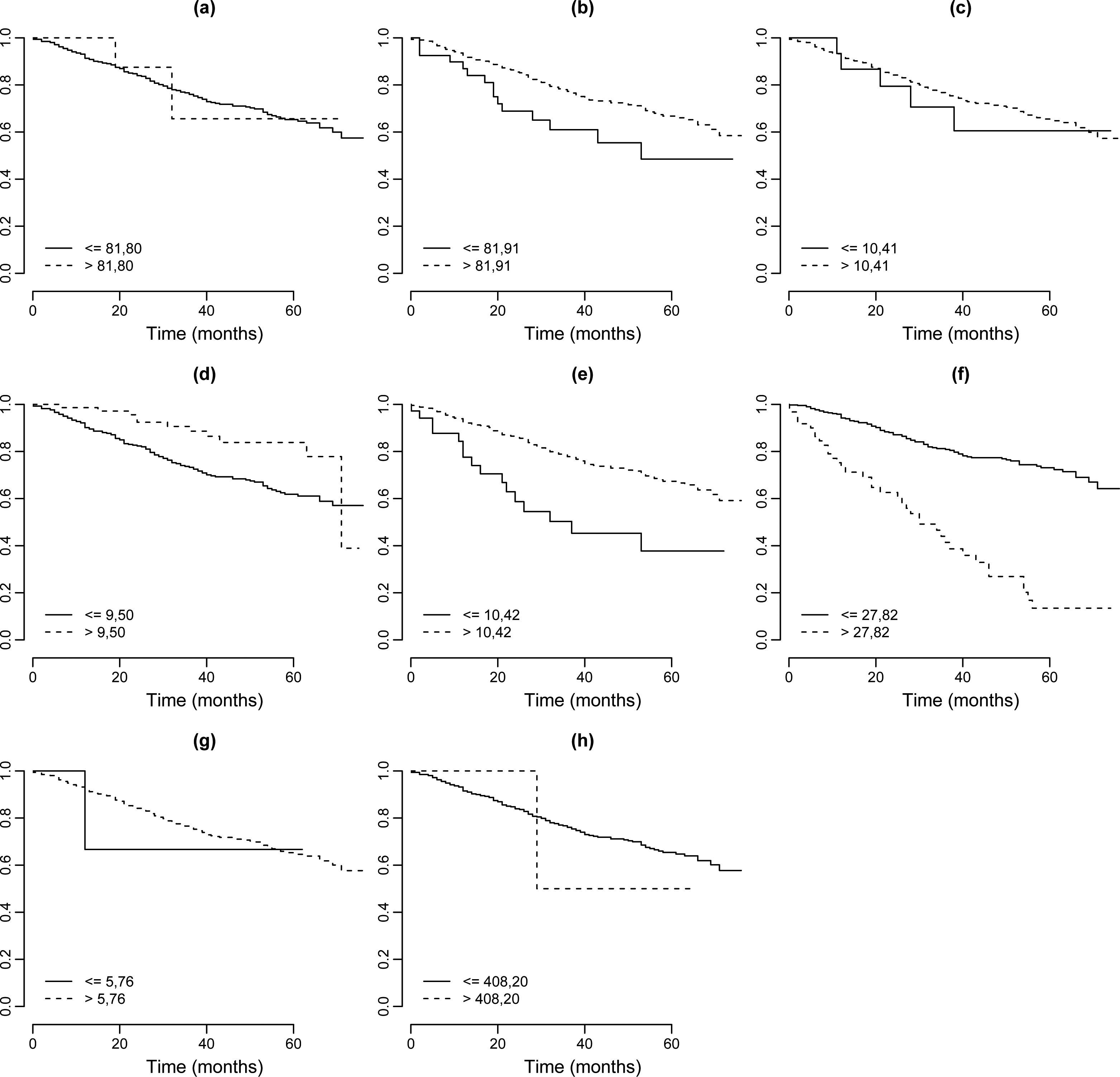

Table 7
Posterior summaries for the Weibull regression model in the presence of cut points (German breast cancer data set)

Mean Standard deviation Median 95% credibility interval

Lower limit Upper limit

Intercept $-$ 10.68 1.00 $-$ 10.75 $-$ 12.19 $-$ 8.07

Age $-$ 1.72 0.68 $-$ 1.69 $-$ 3.27 $-$ 0.53

Menopause 0.15 0.16 0.14 $-$ 0.16 0.46

Hormone $-$ 0.41 0.17 $-$ 0.41 $-$ 0.75 $-$ 0.09

Size 0.54 0.55 0.55 $-$ 0.72 1.54

Grade 0.16 0.15 0.16 $-$ 0.14 0.46

Nodes 1.00 0.16 1.00 0.68 1.33

Prog_recp $-$ 1.23 0.22 $-$ 1.23 $-$ 1.65 $-$ 0.80

Estrg_recp $-$ 0.17 0.22 $-$ 0.18 $-$ 0.56 0.31

Shape 1.51 0.10 1.51 1.32 1.68

$\zeta 1$ age 26.59 3.07 26.62 21.14 31.21

$\zeta 2$ size 67.74 31.21 64.89 13.92 118.30

$\zeta 3$ nodes 3.69 0.62 3.57 3.03 4.89

$\zeta 4$ prog.recp 51.29 76.62 36.47 21.70 133.70

$\zeta 5$ estrg.recp 67.97 83.31 47.14 5.68 223.60

Figure 7.
Histograms for the simulated Gibbs samples of the cut points (Weibull regresssion model – German breast cancer data set).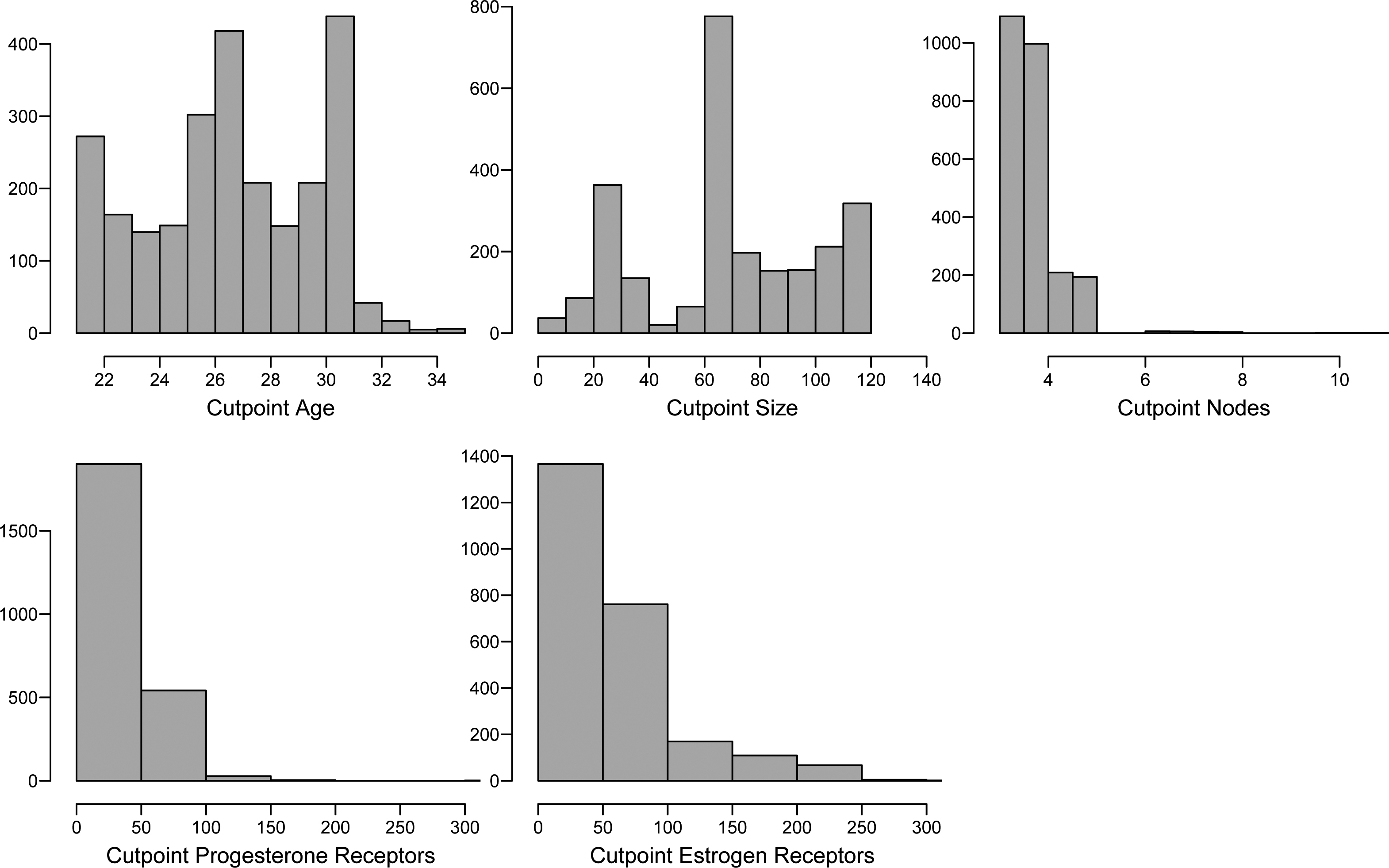

Figure 8.
Plots of Kaplan-Meier estimates for dichotomized covariates, (a) Age; (b) Tumour size in mm; (c) Number of nodes; (d) Number of progesterone receptors; (e) Number of estrogen receptors.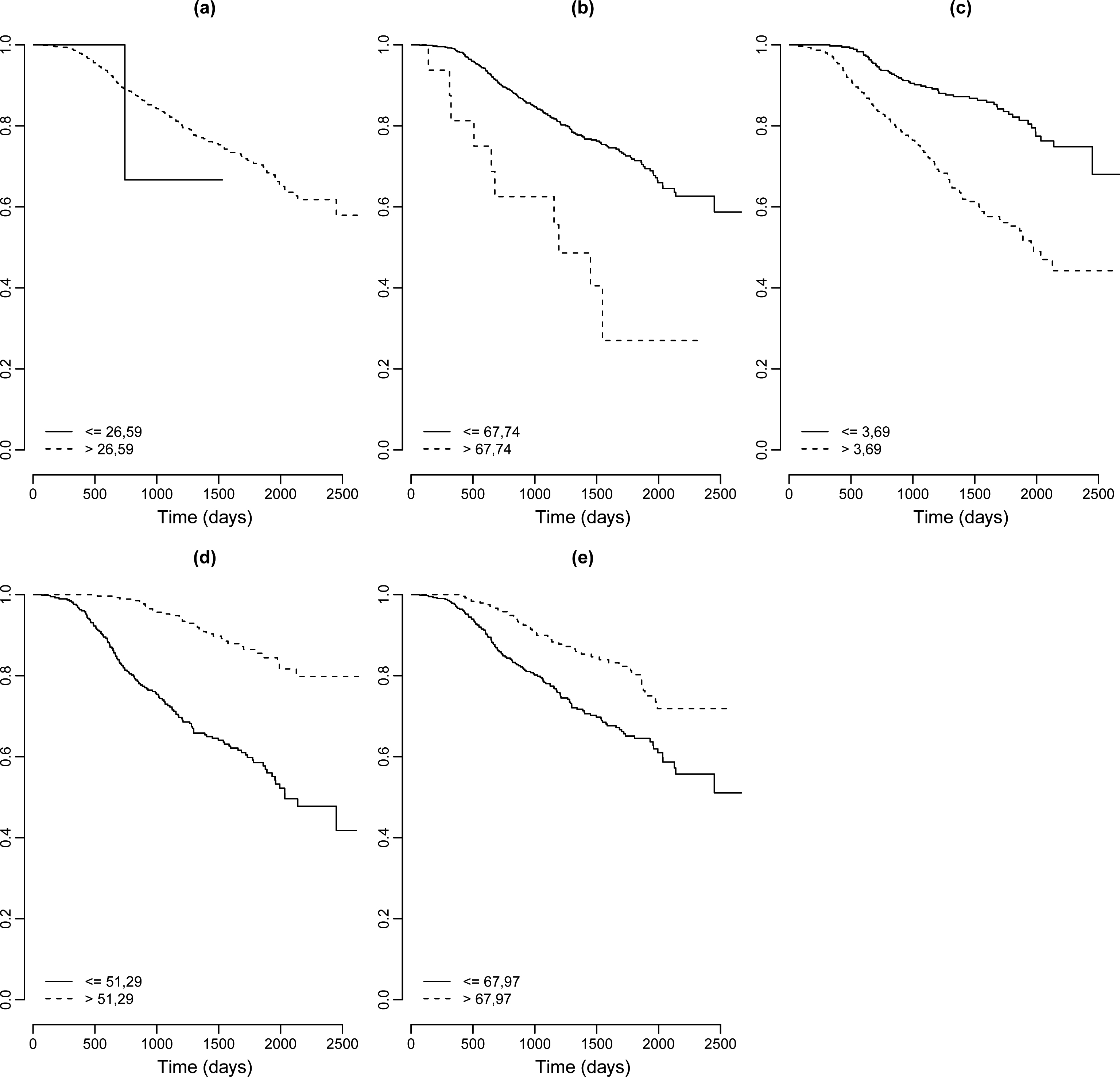

In the same way as considered in application 1 (see Eq. (16)), it is assumed the model in presence of cutpoints given by,

$\displaystyle\gamma_{i}=\exp[\eta_{0}+\eta_{1}x_{1i}+\eta_{2}I_{[0,\tau_{1}]}(% x_{2i})+\eta_{3}I_{[0,\tau_{2}]}(x_{3i})+\eta_{4}x_{4i}+\eta_{5}I_{[0,\tau_{3}% ]}(x_{5i})+\eta_{6}I_{[0,\tau_{4}]}(x_{6i})+\eta_{7}I_{[0,\tau_{5}]}(x_{7i})+% \eta_{8}I_{[0,\tau_{6}]}(x_{8i})+\eta_{9}I_{[0,\tau_{7}]}(x_{9i})+\eta_{10}I_{% [0,\tau_{8}]}(x_{10i})+\eta_{11}x_{11i}+\eta_{12}(x_{12i})]$ (18)

and the prior distributions: $\alpha\sim G(1,1)$ , $\eta_{0}\sim N(5,10)$ , $\eta_{l}\sim N(0,1)$ for $l=1,2,\ldots,12$ ; $\zeta_{1}\sim U(48,89)$ , $\zeta_{2}\sim U(69,152)$ , $\zeta_{3}\sim U(8,30)$ , $\zeta_{4}\sim U(4,18)$ , $\zeta_{5}\sim U(5.9,18.2)$ , $\zeta_{6}\sim U(0,69)$ , $\zeta_{7}\sim U(5,15)$ and $\zeta_{8}\sim U(0.1,999.9)$ using the information of Table 1 to choose the intervals in the uniform priors for the cut points. Further it was assumed independence among the parameters.

Figure 9.
Trace plots of the simulated Gibbs samples for each parameter (application 4.1 An application with a multiple myeloma uncensored data).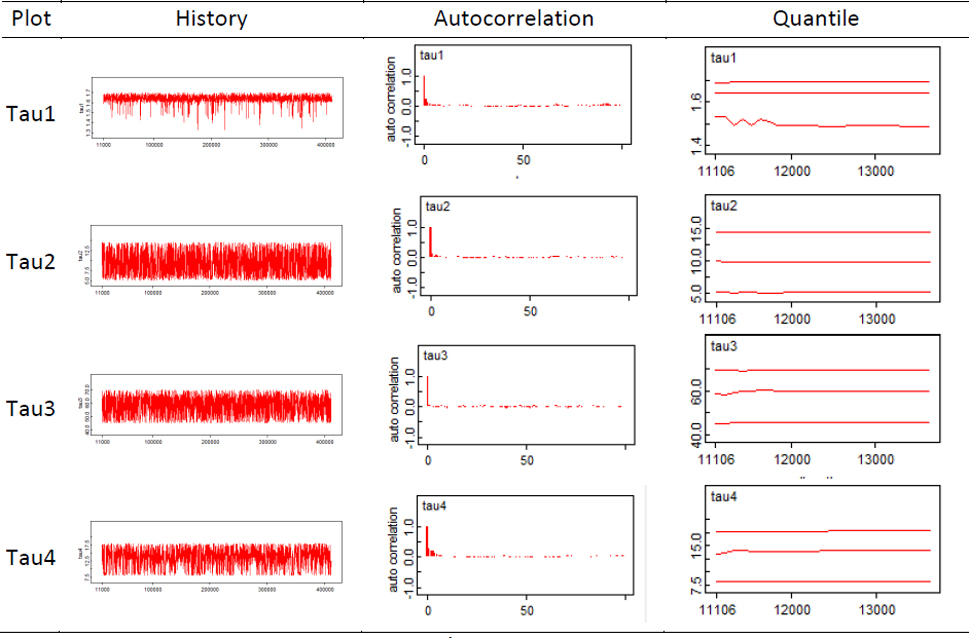

Also observe that the cut points $\zeta_{1}$ , $\zeta_{2}$ , $\zeta_{3}$ , $\zeta_{4}$ , $\zeta_{5}$ , $\zeta_{6}$ , $\zeta_{7}$ and $\zeta_{8}$ are associated to the continuous covariates age, weight index, systolic, diastolic, serum hemogl, sz, sg and ap. The covariates stage, carddisease, bm and rx are discrete variables.

In Table 5, it is presented the posterior summaries of interest (Monte Carlo estimates for the posterior mean, posterior median, posterior standard deviation and 95% credibility intervals for each parameter).

From the results of Table 5, it is concluded that the binary covariates with significative effects on the lifetimes (95% credibility intervals not including the value zero) for patients with prostate cancer are: stage, serum hemogl, sz, sg, bm and rx. The cut points for the continuous covariates are respectively estimated by: 81.80 (age), 81.91 (weight index), 10.41 (systolic), 9.50 (diastolic), 10.42 (serum hem), 27.82 (sz) and 5.76 (sg).

In Fig. 5, it is presented the histograms of the simulated Gibbs samples for the cut points assuming a Weibull regression model. From the graphs of Fig. 5 it is observed that for some cut points as for example, cut points $\zeta_{5}$ and $\zeta_{6}$ associated to the covariates serum hemogl and sz, there is very accurate Bayesian inferences. That is, the proposed approach, even in the presence of censored data is able to capture good estimates for the cut points of the continuous covariates, especially when these covariates have some significative effects on the lifetimes.

Given the cut points for continuous covariates in Table 5, Kaplan-Meier survival curves are estimated for each covariate dichotomized. From the graphs of Fig. 6, it is possible to observe that the covariates weight, diastolic blood pressure, serum prostatic acid phosphatase and size of primary tumor have distinct groups at survival times.

Assuming the dichotomized covariates, Table 4 (b) presents the maximum likelihood estimates (MLE) for the parameters. From the results of Table 4 (b), it is concluded that the dichotomized covariates with significative effects on the lifetimes for patients with prostate cancer are:

•
Significative at 5% ( $p$ -value $<$ 0.05): Serum hemogl, sz, sg, bm, rx,
•
Significative at 10% ( $p$ -value $<$ 0.10): Stage, age and also the diastolic.

4.3 An application with a breast cancer lifetime censored data set

	(a) Continuos covariates	(b) Dichotomized covariates
Predictor	Coefficient	$p$ -value	95% normal CI	Coefficient	$p$ -value	95% normal CI
			Lower limit	Upper limit			Lower limit	Upper limit
Intercept	8.93	0.0000	8.11	9.74	7.53	0.0000	6.27	8.78
Age	0.00	0.5730	$-$ 0.02	0.01	0.95	0.1090	$-$ 0.21	2.11
Menopause	$-$ 0.06	0.7000	$-$ 0.35	0.23	$-$ 0.14	0.1540	$-$ 0.33	0.05
Hormone	0.17	0.0849	$-$ 0.02	0.36	0.19	0.0495	0.00	0.38
Size	$-$ 0.01	0.0054	$-$ 0.01	0.00	$-$ 0.52	0.0081	$-$ 0.90	$-$ 0.14
Grade 2	$-$ 0.46	0.0701	$-$ 0.95	0.04	$-$ 0.28	0.2600	$-$ 0.78	0.21
Grade 3	$-$ 0.67	0.0105	$-$ 1.19	$-$ 0.16	$-$ 0.48	0.0696	$-$ 0.99	0.04
Nodes	$-$ 0.03	0.0000	$-$ 0.04	$-$ 0.02	$-$ 0.63	0.0000	$-$ 0.82	$-$ 0.43
Prog_recp	0.00	0.0000	0.00	0.00	0.70	0.0000	0.44	0.96
Estrg_recp	0.00	0.6840	0.00	0.00	0.11	0.3280	$-$ 0.11	0.34
Shape	$-$ 0.53	0.0000			$-$ 0.54	0.0000

	Mean	Standard deviation	Median	95% credibility interval
Intercept	$-$ 10.68	1.00	$-$ 10.75	$-$ 12.19	$-$ 8.07
Age	$-$ 1.72	0.68	$-$ 1.69	$-$ 3.27	$-$ 0.53
Menopause	0.15	0.16	0.14	$-$ 0.16	0.46
Hormone	$-$ 0.41	0.17	$-$ 0.41	$-$ 0.75	$-$ 0.09
Size	0.54	0.55	0.55	$-$ 0.72	1.54
Grade	0.16	0.15	0.16	$-$ 0.14	0.46
Nodes	1.00	0.16	1.00	0.68	1.33
Prog_recp	$-$ 1.23	0.22	$-$ 1.23	$-$ 1.65	$-$ 0.80
Estrg_recp	$-$ 0.17	0.22	$-$ 0.18	$-$ 0.56	0.31
Shape	1.51	0.10	1.51	1.32	1.68
$\zeta 1$ age	26.59	3.07	26.62	21.14	31.21
$\zeta 2$ size	67.74	31.21	64.89	13.92	118.30
$\zeta 3$ nodes	3.69	0.62	3.57	3.03	4.89
$\zeta 4$ prog.recp	51.29	76.62	36.47	21.70	133.70
$\zeta 5$ estrg.recp	67.97	83.31	47.14	5.68	223.60

In this example, it is considered a lifetime dataset related to the German Breast Cancer Study Data (gbcs.dat) consisting of 686 observations (dataset available in Hosmer et al., 2008). Also available at the Wiley’s FTP site: ftp//ftp.wiley.com/public/sci_tech_med/survival.

In this study, it is only assumed the response survival times in days (0 $=$ censored; 1 $=$ death) and the following covariates:

1.
Age in years (age at diagnosis);
2.
Menopause (1 $=$ yes; 0 $=$ no);
3.
Hormone (hormone therapy; 1 $=$ yes; 0 $=$ no);
4.
Size (tumour size in mm);
5.
Grade (tumour grade; 1,2,3);
6.
Nodes (number of nodes; 1 to 51);
7.
prog. recp (number of progesterone receptors; 1 to 2380);
8.
estrg. recp (number of estrogen receptors; 1 to 1144).

It is assumed as continuous covariates (in some cases the covariates are really not continuous) the variables age, size, nodes, prog.recp and estrg.recp. The dataset has 171 uncensored lifetimes (death from breast cancer) and 515 right censored values (alive or death from other causes).

Once again, the Weibull regression model Eq. (10) it is assumed for the scale parameter $\lambda$ not considering the presence of cutpoints, with the following covariates: $X_{1}=$ age, $X_{2}=$ menopause, $X_{3}=$ hormone, $X_{4}=$ size, $X_{5}=$ grade, $X_{6}=$ nodes, $X_{7}=$ prog recp and $X_{8}=$ estrg recp. The maximum likelihood estimation method (MLE) for the parameters of the model are given in Table 6 (a).

From the results of Table 6 (a), it is concluded that the covariates with significative effects on the lifetimes for patients with breast cancer are:

•
Significative at 5% ( $p$ -value $<$ 0.05): Size, nodes and prog recp,
•
Significative at 10% ( $p$ -value $<$ 0.10): Hormone and grade.

With the same empirical Bayesian approach (use of descriptive summaries for the choice of priors for the cut points given in Table 1) used in example 4.2, the posterior means for the cut points are given in Table 7: age $=$ 26.59 with a 95% credible interval given by (21.14; 31.21); estr.recp $=$ 67.97 with a 95% credible interval given by (5.68; 223.60); node $=$ 3.69 with a 95% credible interval given by (3.03; 4.89); prog.recp $=$ 51.29 with a 95% credible interval given by (21.70; 133.70); and size $=$ 67.74 with corresponding 95% credible intervals given by (13.92; 118.30).

In Fig. 7, it is presented the histograms of the simulated Gibbs samples for the cut points assuming a Weibull regression model. From the graphs of Fig. 7, it is observed that for the cut points associated to the covariates size, nodes, estr.recp and prog.recp there are very accurate Bayesian inferences. That is, the proposed approach, even in the presence of censored data is able to capture good estimates for the cut points of the continuous covariates, especially when these covariates have some significative effects on the lifetimes.

Based on the cut points given in Table 7, Kaplan-Meier survival curves are estimated for each dichotomized covariate.

From the graphs of Fig. 8, it is possible to observe that the covariates size, nodes, number of progesterone receptors and number of estrogen receptors have distinct groups at survival times.

From the results of Table 6 (b), it is concluded that the hormone therapy, tumour size, number of nodes and number of progesterone receptors has significative effect and tumour grade has no more a significative effect on the lifetimes for the patients with breast cancer (significative at 5%, since $p$ -value $<$ 0.05).
5. Concluding remarks

The estimation of optimum cut points for covariates in lifetime regression models is of great interest under a medical view. Despite the loss of information when using a dichotomizing of an independent variable under a regression modeling approach, these cut points are very useful to better diagnosis in different medical situations. One of these applications is given when the medical doctors want to find cut points in covariates which affect the lifetimes of the patients. It is interesting to point out that the lifetime data could be, besides the common situation of lifetime until death, be associated to many other events of interest, as for example, the time of recovery following a medical treatment, the time of a recurrent event, the time of effect of a drug among many others.

The proposed methodology could be used to different lifetime distributions in the AFT model Eq. (3) assuming censored or uncensored data under a Bayesian approach and using MCMC simulation methods.

The computational simulation approach using MCMC methods is greatly simplified using existing simulation free available softwares like the Open Bugs software.

Footnotes

Conflict of interest

The authors declare that there is no conflict of interest.

Appendix A. Open Bugs code

iii. i.

Uncensored data (Krall Data set)

model{ for(i in 1 : N) { time[i] ∼ dweib(r, mu[i]) mu[i] <- exp(beta0+beta1*step(x1[i]-tau1)+ beta2*step(x2[i]-tau2) + beta3*step(x3[i]-tau3)+ beta4*x4[i] + beta5*step(x5[i]-tau4)) } r ∼ dgamma(1,1) beta0 ∼ dnorm(1,0.1) beta1 ∼ dnorm(0,1) beta2 ∼ dnorm(0,1) beta3 ∼ dnorm(0,1) beta4 ∼ dnorm(0,1) beta5 ∼ dnorm(0,1) tau1 ∼ dunif(1.3,1.7) tau2 ∼ dunif(5,14.6) tau3 ∼ dunif(45,70) tau4 ∼ dunif(8,18) }

A Graphical model for this model:

ii.

Grenne e Byar Data set

model{ for(i in 1 : N) { dtime[i] ∼ dweib(r, mu[i])I(cen[i],) mu[i] <- exp(beta0+beta1*stage[i]+beta2*step(age[i]-tau1)+beta3* step(weightindex[i]-tau2)+beta4*carddisease[i]+beta5* step(systolic[i]-tau3)+beta6*step(diastolic[i]-tau4)+beta7* step(serum.hemogl[i]-tau5)+beta8*step(sz[i]-tau6)+beta9* step(sg[i]-tau7)+beta10*step(ap[i]-tau8)+beta11*bm[i]+beta12* rx[i]) } r ∼ dgamma(1,1) beta0 ∼ dnorm(5,0.1) beta1 ∼ dnorm(0,1) beta2 ∼ dnorm(0,1) beta3 ∼ dnorm(0,1) beta4 ∼ dnorm(0,1) beta5 ∼ dnorm(0,1) beta6 ∼ dnorm(0,1) beta7 ∼ dnorm(0,1) beta8 ∼ dnorm(0,1) beta9 ∼ dnorm(0,1) beta10 ∼ dnorm(0,1) beta11 ∼ dnorm(0,1) beta12 ∼ dnorm(0,1) tau1 ∼ dunif(48,89) tau2 ∼ dunif(69,152) tau3 ∼ dunif(8,30) tau4 ∼ dunif(4,18) tau5 ∼ dunif(5.9,18.2) tau6 ∼ dunif(0,69) tau7 ∼ dunif(5,15) tau8 ∼ dunif(0.1,999.9) }

iii.

German breast cancer Data set

model{ for(i in 1 : N) { time[i] ∼ dweib(r, mu[i])I(cen[i],) mu[i] <- exp(beta0+beta1*step(age[i]-tau.age)+beta2*menopause[i]+ beta3*hormone[i]+beta4*step(size[i]-tau.size)+beta5*grade[i]+ beta6*step(node[i]-tau.node)+beta7*step(progrecp[i]-tau.progrecp) +beta8*step(estrrecp[i]-tau.estrrecp)) } r ∼ dgamma(1,1) beta0 ∼ dnorm(8,0.1) beta1 ∼ dnorm(0,1) beta2 ∼ dnorm(0,1) beta3 ∼ dnorm(0,1) beta4 ∼ dnorm(0,1) beta5 ∼ dnorm(0,1) beta6 ∼ dnorm(0,1) beta7 ∼ dnorm(0,1) beta8 ∼ dnorm(0,1) tau.age ∼ dunif(21,80) tau.size ∼ dunif(3,120) tau.node ∼ dunif(1,51) tau.progrecp ∼ dunif(0,2380) tau.estrrecp ∼ dunif(0,1144) }

References

Abdolell

LeBlanc.

Stephens

, & Harrison

R. V.

(2002). Binary partitioning for continuous longitudinal data: Categorizing a prognostic variable. Stat Med, 21(22), 3395-409.

Andrei

A. C.

, & Murray

(2007). Regression models for the mean of the quality-of-life-adjusted restricted survival time using pseudo-observations. Biometrics, 63, 398-404.

Andrews

D. F.

, & Herzberg

A. M.

(1985). Data. New York: Springer-Verlag, and (lib.stat.cmu.edu).

Altman

D. G.

(1991). Categorising continuous variables. British Journal of Cancer, 64, 975.

Altman

D. G.

(1998). Suboptimal analysis using ‘optimal’ cut points. British Journal of Cancer, 78(4), 556-557.

Altman

D. G.

Lausen

Sauerbrei

, & Schumacher

(1994). Dangers of using “optimal” cut points in the evaluation of prognostic factors. Journal of the National Cancer Institute, 86, 829-835.

Altman

D. G.

, & Royston

(2006). The cost of dichotomizing continuous variables. BMJ, 332(7549), 1080.

Box

G. E. P.

, & Tiao

(1973). Bayesian inference in statistical analysis. New York: Addison-Wesley.

Carlin

B. P.

, & Louis

T. A.

(1996). Bayes and empirical Bayes methods for data analysis. Chapman & Hall, London, 397.

10.

Chib

, & Greenberg

(1995). Understanding the Metropolis-Hastings algorithm. The American Statistician, 49(4), 327-335.

11.

Collett

(2003). Modelling Survival Data in Medical Research, 2nd edition. Chapman and Hall/CRC.

12.

Contal

, & O’Quigley

(1999). An application of change-point methods in studying the effect of age on survival in breast cancer. Computational Statistics and Data Analysis, 30, 253-270.

13.

Cox

D. R.

(1972). Regression models and life tables. Journal of the Royal Statistical Society B, 34, 187-220.

14.

Cumsille

Bangdiwala

S. I.

Sen

P. K.

, & Kupper

L. L.

(2000). Effect of dichotomizing a continuous variable on the model structure in multiple linear regression models. Communications and Statistics – Theory and Methods, 29, 643-654.

15.

Gelfand

A. E.

, & Smith

A. F. M.

(1990). Sampling based approaches to calculating marginal densities. Journal of the American Statistical Association, 85(410), 398-409.

16.

Green

K. R.

, & Byar

D. P.

(1980). Treatment effects in competing-risks analysis of prostate cancer data. Bulletin Cancer, 67, 477-488.

17.

Gumbel

E. J.

(1954). Statistical theory of extreme values and some practical applications. Applied Mathematics, Series 33, U.S. Department of Commerce, National Bureau of Standards.

18.

Hilsenbeck

S. G.

, & Clark

G. M.

(1996). Practical p-value adjustment for optimally selected cut points. Statistics in Medicine, 15(1), 103-112.

19.

Hollander

, & Schumacher

(2001). On the problem of using ‘optimal’ cut points in the assessment of quantitative prognostic factors. Onkologie, 24(2), 194-199.

20.

Hollander

Sauerbrei

, & Schumacher

(2004). Confidence intervals for the effect of a prognostic factor after selection of an ‘optimal’ cutpoint. Statistics in Medicine, 23, 170-713.

21.

Hosmer

D. W.

Lemeshow

, & May

(2008). Applied Survival Analysis: Regression Modeling of Time to Event Data: Second Edition. John Wiley and Sons Inc., New York, NY.

22.

Jespersen

N. C. B.

(1986). Dichotomizing a continuous covariate in the Cox regression model. Statistical Research Unit of University of Copenhagen, Research Report, 86(2).

23.

Kalbfleisch

J. D.

, & Prentice

R. L.

(2002). The Statistical Analysis of Failure Time Data, 2nd Edition. John Wiley and Sons, Hoboken, New Jersey.

24.

Kaplan

E. L.

, & Meier

(1958). Nonparametric estimation from incomplete observations. Journal of the American Statistical Association, 53, 457-481.

25.

Klein

J. P.

, & Moeschberger

M. L.

(2003). Survival Analysis, Techniques for Censored and Truncated Data, 2nd Edition. Springer, New York.

26.

Klein

J. P.

, & Wu

J. T.

(2004). Discretizing a continuous covariate in survival studies. In: Balakrishnan N, Rao CR, editors. Handbook of Statistics 23: Advances in Survival Analysis. New York: Elsevier, 27-42.

27.

Krall

Uthof

, & Harley

(1975). A step-up procedure for selecting variables associated with survival. Biometrics, 31, 49-57.

28.

Lausen

Hothorn

Bretz

, & Schumacher

(2004). Assessment of optimal selected prognostic factors. Biometrical Journal, 46(3), 364-374.

29.

Lausen

, & Schumacher

(1992). Maximally selected rank statistics. Biometrics, 48, 73-85.

30.

Lausen

, & Schumacher

(1996). Evaluating the effect of optimized cutoff values in the assessment of prognostic factors. Computational Statistics and Data Analysis, 21, 307-326.

31.

Lawless

J. F.

(1982). Statistical models and methods for lifetime data. Wiley Series in Probability and Mathematical Statistics, Wiley & Sons.

32.

Lee

E. T.

, & Wenyuwang

(2003). Statistical methods for survival data analysis, Third Edition. John Wiley & Sons, New Jersey.

33.

Liquet

, & Commenges

(2001). Correction of the p-value after multiple coding of an explanatory variable in logistic regression. Statistics in Medicine, 20, 2815-2826.

34.

MacCallum

R. C.

Zhang.

Preacher

K. J.

, & Rucker

D. D.

(2002). On the practice of dichotomization of quantitative variables. Psychol Methods, 7(1), 19-40.

35.

Magder

L. S.

, & Fix

A. D.

(2003). Optimal choice of a cut point for a quantitative diagnostic test performed for research purposes. Journal of Clinical Epidemiology, 56, 956-962.

36.

Mazumdar

Smith

, & Bacik

(2003). Methods for categorizing a prognostic variable in a multivariable setting. Statistics in Medicine, 22(4), 559-71.

37.

Mazumdar

Glassman

J. R.

(2000). Categorizing a prognostic variable: Review of methods, code for easy implementation and applications to decision-making about cancer treatments. Statistics in Medicine, 19, 113-132.

38.

Meeker

W. Q.

, & Escobar

L. A.

(1998). Statistical Methods for Reliability Data, 2nd Edition. John Wiley and Sons, Hoboken, New Jersey.

39.

Nelson

(2004). Applied life data analysis. Wiley – Blackwell.

40.

Ragland

D. R.

(1992). Dichotomizing continuous outcome variables: Dependence of the magnitude of association and statistical power on the cutpoint. Epidemiology, 3, 434-440.

41.

Silva

G. T.

Klein

J. P.

(2011). Cutpoint selection for discretizing a continuous covariate for generalized estimating equations. Computational Statistics and Data Analysis, 55(1), 226-235.

42.

Spiegelhalter

D. J.

Thomas

Best

N. G.

, & Lunn

(2003). WinBugs version 1.4 user manual. Institute of Public Health and Department of Epidemiology & Public Health, London. (http://www.mrc-bsu.com.ac.uk/bugs).

43.

Spiegelhalter

D. J.

Best

N. G.

Carlin

B. P.

LindeVan der

(2002). Bayesian measures of model complexity and fit (with discussion). Journal of the Royal Statistical Society B, 583-639.