Semiparametric transformation model:A hierarchical Bayesian approach

Abstract

The use of semiparametric or transformation models has been considered by many authors in the analysis of lifetime data in the presence of censoring and covariates as an alternative and generalization of the usual proportional hazards, the proportional odds models, and the accelerated failure time models, extensively used in lifetime data analysis. The inferences for the proportional hazards model introduced by Cox (1972) are usually obtained by maximum likelihood estimation methods assuming the partial likelihood function introduced by Cox (Cox, 1975). In this study, we consider a hierarchical Bayesian analysis of the proportional hazards model assuming the complete likelihood function obtained from a transformation model considering the unknown hazard function as a latent unknown variable under a Bayesian approach. Some applications with real time medical data illustrate the proposed methodology.

Keywords

Lifetime data semiparametric models censored data covariates hierarchical Bayesian analysis MCMC methods

1. Introduction

Lifetime data often presents censored observations and covariates associated with each individual. Different parametric or non-parametric regression models are introduced in the literature to analyze lifetime data in the presence of censoring and covariates (Lawless, 1982; Klein & Moeschberger, 1997; Cox & Oakes, 1984). Three classes of models have been extensively used in lifetime data analysis in the presence of censoring and covariates: the proportional hazards or PH models (Cox, 1972), the proportional odds or PO models (Bennett, 1983), and accelerated failure time or AFT models (Kalbfleisch and Prentice, 2002). In many situations, these models could be not suitable with crossing survival curves. Some earlier generalizations of these models, including the PH and PO models, could be seen in the literature as the semiparametric two-sample strategy (YP model) proposed by Yang and Prentice (2005). A unified approach to fit the YP model is introduced by Demarqui et al. (2019) using Bernstein polynomials to manage the baseline hazard and odds under both the frequentist and Bayesian frameworks.

In many applications of survival analysis, the class of accelerated failure time models is useful to model the relationship between failure times and the associated covariates, where covariate effects are assumed to appear in a linear form, which could be restrictive for many practical problems (Lawless, 1982). To incorporate flexible nonlinear relationships between covariates and transformed failure times, He and Yi (2020) propose parametric and semiparametric estimation methods for survival data under a flexible class of models.

A popular methodology extensively used in medical applications in the analysis of survival data that incorporates the introduction of covariates is the popular proportional hazards (PH) model introduced by Cox (1972). The Cox model is a semi-parametric model of easy and simple interpretation where the occurrence of censorship is easily accommodated. In addition, it is available in most statistical software. The Cox model assumes that the hazard function can be written in the form,

$\displaystyle h(t;\bm{z})=h_{0}(t)e^{\bm{\beta}\bm{z}}$ (1)

where $t$ is the value of a random variable $T>0$ denoting the lifetime of one unit, $h_{0}(t)$ is a non-negative arbitrary baseline hazard function defined as the limit of the probability of an individual to failure in the interval $[t,t+\Delta t]$ given that this individual is surviving until time $t$ , that is,

$\displaystyle h(t)=\lim_{\Delta t\to 0}\frac{P(t\leqslant T<t+\Delta t\mid T% \geqslant t)}{\Delta t},$ (2)

$\bm{\beta}$ is a vector of regression coefficients and $\bm{z}$ is a vector of covariates.

Under this model, the ratio of hazard functions for two different individuals with fixed covariate vectors is constant in time (proportional hazards model), that is, not dependent on time. The two multiplicative components of the model Eq. (1) are of different natures, one is non-parametric and the other is parametric (a semi-parametric model). The covariates affect the hazard function in a multiplicative way according to the factor $e^{\bm{\beta}\bm{z}}$ . Cox (1972) proposed a likelihood function that does not depend on the baseline hazard function $h_{0}(t)$ , thus allowing inferences on $\bm{\beta}$ without the need to specify $h_{0}(t)$ .

Considering $n$ individuals under study and $k$ distinct moments of observation of the event of interest (e.g., deaths), such that $t_{1}<t_{2}<\ldots<t_{k}$ , where $k\leqslant n$ , the partial (or marginal) likelihood function, proposed by Cox (1972) is given by

$\displaystyle L(\bm{\beta})=\prod_{i=1}^{k}\frac{e^{\beta z_{i}}}{% \displaystyle\sum_{l\in R_{i}}e^{\beta z_{l}}}$ (3)

where $R_{i}$ is the set of individuals at risk over time $t_{i}$ , and $\bm{z}_{i}$ is the vector of explanatory variables associated with the individual having the event of interest at time $t_{i}$ . Cox (1975) showed that, although Eq. (3) it is not a likelihood function in the usual sense, under very general conditions, it is verified the usual properties of the maximum likelihood estimators. Note that the likelihood function proposed by Cox (1975) does not depend on $h_{0}(t)$ , which allows for inferences on the vector of parameters $\bm{\beta}$ , without having to make restrictions on the form of $h_{0}(t)$ . As Cox (1975) has shown, the partial likelihood construction method, under fairly weak regularity conditions, leads to the usual asymptotic properties of likelihood-based inference.

In recent years, some generalizations of the proportional hazards models were introduced in the literature. Li et al. (2021) introduced a model averaging method to produce model-based prediction for survival outcomes defined as a semiparametric model averaging prediction (SMAP) method which approximates the underlying unstructured nonparametric regression function by a weighted sum of low-dimensional nonparametric submodels. The weights are obtained from maximizing the partial likelihood constructed for the aggregated model and theoretical properties are discussed for the estimated model weights.

Race and Pennell (2021) introduced a semi-parametric survival analysis via Dirichlet process mixtures of the First Hitting Time (FHT) model, considering several random effects specifications of the FHT model under a Bayesian approach.

Yang and Niu (2021) introduced semi-parametric models for longitudinal data analysis. Zhou et al. (2017) considered semiparametric transformation models for interval-censored data.

Selingerova et al. (2021) introduced a study for the comparison of parametric and semiparametric survival regression models with kernel estimation considering two types of kernel smoothing and some bandwidth selection techniques. An overview of semiparametric models commonly used in survival analysis, including proportional hazards model, proportional odds models and linear transformation models was introduced by Guo and Zeng (2014). Many other studies are introduced in the literature: Lin and Ying (1994) assumed the additive risk model specifying that the hazard function associated with a set of possibly time-varying covariates is the sum of the baseline hazard function and the regression function of covariates in contrast to the usual proportional hazards model; Lin et al. (2000) considered in place of the usual Cox-type intensity function for counting process commonly used to analyse recurrent event data, a time-transformed Poisson process assuming that the covariates have multiplicative effects on the mean and rate functions of the counting process; Race and Pennell (2021) assumed a model derived from the First Hitting Time (FHT) paradigm which assumes that a subject’s event time is determined by a latent stochastic process reaching a threshold value for better modeling of data with unmeasured covariates proposing a Bayesian model which loosens assumptions on the mixing distribution inherent in the random effects FHT models currently in use; Ma and Kosorok (2005) considered partly linear transformation models (semiparametric regression models) applied to current status data where the unknown quantities are the transformation function, a linear regression parameter and a nonparametric regression effect showing flexible alternatives to the Cox model for current status data analysis; Rossini and Tsiatis (1996) introduced a covariate analysis of current status data showing that the method is applicable when the logit of the conditional probability of survival given the covariates is some increasing function of time plus a linear combination of the covariates; Song et al. (2002) investigated joint models for a time-to-event (e.g., survival) and a longitudinal response where the longitudinal data are assumed to follow a mixed effects model and a proportional hazards model depending on the longitudinal random effects and other covariates are assumed for the survival endpoint proposing a likelihood-based approach that requires only the assumption that the random effects have a smooth density; Song and Wang (2008) studied joint modeling of survival and longitudinal data where there are two regression models of interest, the first one for survival outcomes, which are assumed to follow a time-varying coefficient proportional hazards model and the second one is for longitudinal data, which are assumed to follow a random effects model proposing a local corrected score estimator and a local conditional score estimator to deal with covariate measurement error; Zeng and Cai (2010) proposed a semiparametric additive rate model for modelling recurrent events in the presence of a terminal event where a general transformation model is used to model the terminal event; Zeng et al. (2005) introduced a new class of transformed hazard rate models that contains both the multiplicative hazards model and the additive hazards model as special cases; Zeng et al. (2008) proposed a general class of semiparametric transformation models with random effects to formulate the effects of possibly time-dependent covariates on clustered or correlated failure times encompassing all commonly used transformation models, including proportional hazards and proportional odds models; Zeng and Lin (2009) proposed a large class of semiparametric transformation models with random effects for the joint analysis of recurrent events and a terminal event where the transformation models include proportional hazards/intensity and proportional odds models.

In this article, we introduce a hierarchical Bayesian analysis of the proportional hazards model assuming the complete likelihood function obtained from a transformation model considering the unknown hazard function as a latent unknown variable under a Bayesian approach. The paper is prepared as follows: in Section 2, we introduce some classes of semiparametric models for lifetime data in presence of censored data and covariates; Section 3 presents the special case considering the use of a special transformation $G(x)=x$ (a proportional hazards model); Section 4 illustrates the proposed methodology considering some examples with medical data. Section 5 shows the results of a simulation study. Finally, Section 6 presents some concluding remarks.

2. Transformation model

Let $T$ denote the failure time, and let $\bm{z}(\cdot)$ denote a d-vector of covariates associated to each individual. Under the semiparametric transformation model, the cumulative hazard function for $T$ conditional on $\bm{z}$ is given by,

$\displaystyle\Lambda(t;\bm{z})=G\left\{\int_{0}^{t}e^{\beta\bm{z}}h(u)du\right\}$ (4)

where $G(\cdot)$ is a specific transformation function that is strictly increasing, $\beta$ is a regression parameter and $\Lambda(\cdot)$ is an unknown increasing function (Zeng et al., 2016) defined by $\Lambda(t)=\int_{0}^{t}h(u)du$ denoting the usual cumulative hazard function not considering the presence of the covariate vector $\bm{z}$ .

Then,

$\displaystyle\Lambda(t;\bm{z})=G\left\{e^{\beta\bm{z}}\Lambda_{0}(t)\right\}$ (5)

where $\Lambda_{0}(t)$ is the baseline cumulative hazard function.

The use of this class of semiparametric models has been recently used by many authors in the analysis of lifetime data in the presence of censoring and covariates. In the presence of a fraction of individuals not experiencing the event of interest (cured or non-susceptible individuals), Chen et al. (2012) introduced a marginal analysis of multivariate failure time data with a surviving fraction based on semiparametric transformation cure models. Some generalizations of the semiparametric model (or transformation models) are also proposed in the literature (Chen et al., 2002, 2012; Sun & Sun, 2005).

Gao et al. (2018) introduced semiparametric regression analysis of interval-censored data with informative dropout, and Zeng et al. (2016) introduced a maximum likelihood estimation approach for semiparametric transformation models in the presence of interval-censored data.

Some special cases of the semiparametric model Eq. (4) are given in the following,

(a)

If $G(x)=x$ , $\Lambda(t;\bm{z})=e^{\beta\bm{z}}\Lambda_{0}(t)$ , where $\Lambda_{0}(t)=\int_{0}^{t}h_{0}(u)du$ ( $h_{0}$ is unknown), that is, we have the proportional hazards model since $h(t;\bm{z})=e^{\beta\bm{z}}h_{0}(t)$ . In this case, two individuals denoted by $i$ and $j$ with covariates $z_{i}$ and $z_{j}$ have a hazard ratio given by $h(t;\bm{z}_{i})/h(t;\bm{z}_{j})=e^{\beta\bm{z}_{i}}h_{0}(t)/e^{\beta\bm{z}_{j}% }h_{0}(t)=e^{\beta z_{i}}/e^{\beta z_{j}}$ (does not depend on $t$ , that is, we have a proportional hazards model).

(b)

If $G(x)=\log(1+x)$ , we have $\Lambda(t;\bm{z})=\log\left\{1+e^{\beta\bm{z}}\Lambda_{0}(t)\right\}$ , $S(t;\bm{z})=\exp\left(-\Lambda(t;\bm{z})\right)=\exp\bigl{(}-\log\linebreak% \left[1+e^{\beta\bm{z}}\Lambda_{0}(t)\right]\bigr{)}=1/\left[1+e^{\beta\bm{z}}% \Lambda_{0}(t)\right]$ and $1-S(t;\bm{z})=e^{\beta\bm{z}}\Lambda_{0}(t)/\left[1+e^{\beta\bm{z}}\Lambda_{0}% (t)\right]$ , ( $S(t)=P(T>t)$ is the survival function) leading to the proportional odds ratio model, since

$\displaystyle\textit{OR}_{i}/\textit{OR}_{j}=\left\{S(t;\bm{z}_{i})/\left[1-S(% t;\bm{z}_{i})\right]\right\}/\left\{S(t;\bm{z}_{j})/\left[1-S(t;\bm{z}_{j})% \right]\right\}=\left\{S(t;\bm{z}_{i})/S(t;\bm{z}_{j})\right\}\left\{\left[1-S% (t;\bm{z}_{j})\right]/\left[1-S(t;\bm{z}_{i})\right]\right\}=\left\{\left[1+e^% {\beta\bm{z}_{j}}\Lambda_{0}(t)\right]/\left[1+e^{{\beta\bm{z_{i}}}}\Lambda_{0% }(t)\right]\right\}\cdot\left\{e^{\beta\bm{z}_{j}}\Lambda_{0}(t)/\left[1+e^{% \beta\bm{z}_{j}}\Lambda_{0}(t)\right]\right\}\cdot\left\{\left[1+e^{\beta\bm{z% _{i}}}\Lambda_{0}(t)\right]/e^{\beta\bm{z_{i}}}\Lambda_{0}(t)\right\}.$

That is, $\textit{OR}_{i}/\textit{OR}_{j}=\left\{e^{\beta\bm{z}_{j}}\Lambda_{0}(t)/e^{% \beta\bm{z}_{i}}\Lambda_{0}(t)\right\}=e^{\beta\bm{z}_{j}}/e^{\beta\bm{z_{i}}}$ (a proportional odds model).

(c)

If $G(x)=\log(1+rx)/r(r\geqslant 0)$ , the logarithmic transformation family, with $G(x)=x$ if $r=0$ and $G(x)=\log(1+x)$ if $r=1$ (Zeng et al., 2016). In this case we have $\Lambda(t;\bm{z}_{i})=\log\left\{1+re^{\beta\bm{z}}\Lambda_{0}(t)\right\}/r$ and $S(t,\bm{z})=\exp(-\Lambda(t,\bm{z}))=\exp\left(-\frac{\log(1+re^{\bm{\beta z_{% i}}}\Lambda_{0}(t))}{r}\right)$ .

The likelihood function in the presence of right-censored data and a vector of covariates $\bm{Z}$ is given by,

$\displaystyle L(\cdot)=\prod_{i=1}^{n}f(\bm{t}_{i};\bm{z}_{i})^{\delta_{i}}S(% \bm{t}_{i},\bm{z}_{i})^{1-\delta_{i}}$ (6)

where $\bm{z}_{i}$ is a vector of covariates; $\delta_{i}=1$ (complete observation) and $\delta_{i}=0$ (censored observation). Since $h(t)=f(t)/S(t)$ , we have $f(t)=h(t)S(t)$ . Thus, the likelihood function [Eq. (6)] can be written as,

$\displaystyle L(\cdot)=\prod_{i=1}^{n}h(t_{i},\bm{z}_{i})^{\delta_{i}}S(t_{i},% \bm{z}_{i}).$ (7)

Remark (some preliminary results)

•

Some relations involving $\Lambda(t),S(t),h(t)$ and $f(t)$ can be obtained from the expression.

$\displaystyle h(t)=\lim_{\Delta t\to 0}\frac{P(t\leqslant T\leqslant t+\Delta t% \mid T\geqslant t)}{\Delta t}=\frac{f(t)}{S(t)}$

We know that $S(t)=P(T\geqslant t)=1-F(t)$ . Then,

$\displaystyle f(t)=\frac{dF(t)}{dt}=\frac{d}{dt}\left(1-S(t)\right).$

Now

$\displaystyle\Lambda(t)=\int_{0}^{t}h(u)du=\int_{0}^{t}\frac{d}{du}\left(1-F(u% )\right)\times\frac{1}{S(u)}du=-\int_{0}^{t}\frac{d}{du}S(u)\times\frac{1}{S(u% )}du=-\ln(S(t)).$

Thus, $S(t)=\exp(-\Lambda(t))$ and we have,

•

The accumulated hazard function $\Lambda(t)$ can be given by $\Lambda(t)=\int_{0}^{t}h(u)du=-\log[S(t)]$ .

•

The hazard function $h(t)$ can be given by $h(t)=d\Lambda(t)/dt=-S^{\prime}(t)/S(t)$ .

•

The density function $f(t)$ can be given by $f(t)=dF(t)/dt$ where $F(t)=1-S(t)$ .

3. A special case: use of the transformation

\bm{G(x)=x}

(a proportional hazards model)

In this case, we have $\Lambda(t;\bm{z})=e^{\beta\bm{z}}\Lambda_{0}(t)$ that is, $h(t;\bm{z})=e^{\beta\bm{z}}h_{0}(t)$ (hazard function). Thus, $S(t;\bm{z})=e^{-\Lambda(t;\bm{z})}=e^{-e^{\beta\bm{z}}\Lambda_{0}(t)}$ , and $f(t;\bm{z})=h(t;\bm{z})S(t;\bm{z})=e^{\beta\bm{z}}h_{0}(t)e^{-e^{\beta\bm{z}}% \Lambda_{0}(t)}$ . Thus, the likelihood function (in the presence of right-censored data and covariates) is given from Eq. (7) by,

$\displaystyle L(\cdot)=\prod_{i=1}^{n}h(t_{i},\bm{z}_{i})^{\delta_{i}}S(t_{i};% \bm{z}_{i})=\prod_{i=1}^{n}\left[e^{\beta\bm{z}_{i}}h_{0}(t_{i})\right]^{% \delta_{i}}e^{-e^{\beta\bm{z}_{i}}\Lambda_{0}(t_{i})}=e^{\sum_{i=1}^{n}\delta_% {i}\beta\bm{z}_{i}}\left\{\prod_{i=1}^{n}\left[h_{0}(t_{i})\right]^{\delta_{i}% }\right\}e^{-\sum_{i=1}^{n}e^{\beta\bm{z}_{i}}\Lambda_{0}(t_{i})}.$ (8)

The log-likelihood function is given by,

$\displaystyle l(\cdot)=\log[L(\cdot)]=\sum_{i=1}^{n}\delta_{i}\beta\bm{z}_{i}+% \sum_{i=1}^{n}\delta_{i}\log[h_{0}(t_{i})]-\sum_{i=1}^{n}e^{\beta\bm{z}_{i}}% \Lambda_{0}(t_{i}).$

Considering the contribution of only one observation $i$ , we have:

$\displaystyle l(\cdot)=\log[L(\cdot)]=\delta_{i}\beta\bm{z}_{i}+\delta_{i}\log% [h_{0}(t_{i})]-e^{\beta\bm{z}_{i}[\Lambda_{0}(t_{i})]}$ (9)

where $h_{0}(t_{i})$ and $\Lambda_{0}(t_{i})$ are unknown.

Remark 1: considering a Weibull distribution, a proportional hazards model, with density $f(t)=[\gamma/\alpha^{\gamma}]t^{\gamma-1}\linebreak e^{-(t/\alpha)^{\gamma}}$ , we have $h_{0}(t)=[\gamma/\alpha^{\gamma}]t^{\gamma-1}$ and $\Lambda_{0}(t)=(t/\alpha)^{\gamma}$ , we get from Eq. (8) the standard likelihood function assuming a Weibull distribution.

Since $h_{0}(t)$ is unknown $(\Lambda_{0}(t)$ is also unknown), we could consider numerical approximations for the hazard function, as a polynomial approximation (Chen et al., 2013) given by, $h_{0}(t)=a_{1}+a_{2}t+a_{3}t^{2}+a_{4}t^{3}+\cdots+a_{k}t^{k-1}$ , that is, $\Lambda_{0}(t)=a_{1}t+a_{2}t^{2}/2+a_{3}t^{3}/3+a_{4}t^{4}/4+\cdots+a_{k}t^{k}/k$ since $d\Lambda_{0}(t)/dt=h_{0}(t)$ . Observe that we must have $h_{0}(t)=a_{1}+a_{2}t+a_{3}t^{2}+a_{4}t^{3}+\cdots+a_{k}t^{k-1}>0$ and $\Lambda_{0}(t)=a_{1}t+a_{2}t^{2}/2+a_{3}t^{3}/3+a_{4}t^{4}/4+\cdots+a_{k}t^{k}% /k>0$ , which implies in some difficulties in the elicitation of prior distributions for the unknown parameters $a_{j}$ , $j=1,2,\cdots,k$ .

As the main goal of this study, we present a hierarchical Bayesian approach (Gelman et al., 2004) for the transformation model $G(x)=x$ (proportion hazard model), since $h_{0}(t)$ could be assumed as a latent unknown random variable. In this way, we assume $d_{i}=h_{0}(t_{i})$ as a random effect, that is, $\Lambda_{0}(t_{i})=d_{i}t_{i}$ assuming a specified probability distribution and a hierarchical Bayesian analysis using standard MCMC (Markov Chain Monte Carlo) methods as the Gibbs sampling algorithm and the Metropolis-Hastings algorithm (Gelfand & Smith, 1990; Chib & Greenberg, 1995). In the special situation with only one covariate $z$ , that is, only one regression parameter $\beta$ [likelihood Eq. (9)], we assume for a hierarchical Bayesian analysis, $d_{i}\sim G(1,\tau_{\lambda}),i=1,2,\cdots,n$ where $G(a,b)$ denotes a gamma distribution with mean $a/b$ and variance $a/b^{2}$ and a gamma prior distribution for the parameter $\theta$ in the first stage of the hierarchical Bayesian approach, that is, $\theta\sim G(a,b)$ , where $\theta=\exp(\beta)$ and $a$ and $b$ are known hyperparameters. In the second stage of the hierarchical Bayesian approach, we assume a uniform distribution for the parameter $\tau_{\lambda}$ , that is, $\tau_{\lambda}\sim U(c,d)$ where $U(c,d)$ denotes a uniform distribution in the interval $(c,d)$ and $c$ and $d$ are known hyperparameters. We assume the reparameterization $\theta=\exp(\beta)$ to have better convergence of the Gibbs sampling algorithm. Considering a vector of covariates associated with a vector of parameters $\bm{\theta}=(\theta_{1},\theta_{2},\theta_{3},\cdots,\theta_{k})$ , $\theta_{j}=\exp(\beta_{j}),j=1,2,\cdots,k$ we assume independent gamma prior distributions $\theta_{j}\sim G(a_{j},b_{j})$ and the same distribution structure $d_{i}\sim G(1,\tau_{\lambda})$ for the latent factor. Alternatively, we could assume independent uniform priors for the parameters $\theta_{j}$ . Under a Bayesian approach, we use the Bayes formula to combine a specified prior distribution for the parameters of the model with the likelihood function of the model, obtaining the posterior distribution from where the Bayesian inferences are obtained. Therefore, for $\bm{\theta}$ , the vector of parameters of a model describing the behavior of the data $D$ , if $P(\bm{\theta}),P(\bm{\theta}\mid D)$ , and $L(D\mid\bm{\theta})$ indicate, respectively, the prior, the posterior distributions of $\bm{\theta}$ , and the likelihood function of the model, then $P(\bm{\theta}\mid D)\propto L(D\mid\bm{\theta})P(\bm{\theta})$ .

4. Applications

4.1 Example 1

The remission times of 42 patients with acute leukemia were reported by Freireich et al. (1963) in a clinical trial conducted to assess the ability of 6-mercaptopurine (6-MP) to maintain remission. Each patient was randomized to receive 6-MP or a placebo. The study finished after one year. The following remission times, in weeks, were recorded: 6-MP (21 patients): 6, 6, 6, 7, 10, 13, 16, 22, 23, 6 $+$ , 9 $+$ , 10 $+$ , 11 $+$ , 17 $+$ , 19 $+$ , 20 $+$ , 25 $+$ , 32 $+$ , 32 $+$ , 34 $+$ , 35 $+$ ; Placebo (21 patients): 1, 1, 2, 2, 3, 4, 4, 5, 5, 8, 8, 8, 8, 11, 11, 12, 12, 15, 17, 22, 23.

Table 1
Kaplan-Meier survival function and cumulative hazard estimates

Row	$t$ (6MP)	$S_{1}(t)$	$\Lambda_{1}(t)$	$t$ (placebo)	$S_{2}(t)$	$\Lambda_{2}(t)$
1	6	0.857	0.154	1	0.905	0.100
2	7	0.807	0.215	2	0.810	0.211
3	10	0.753	0.284	3	0.762	0.272
4	13	0.690	0.371	4	0.667	0.405
5	16	0.628	0.466	5	0.571	0.560
6	22	0.538	0.620	8	0.381	0.965
7	23	0.448	0.803	11	0.286	1.253
8				12	0.190	1.658
9				15	0.142	1.946
10				17	0.095	2.351
11				22	0.048	3.045
12				23	0.000

Figure 1.

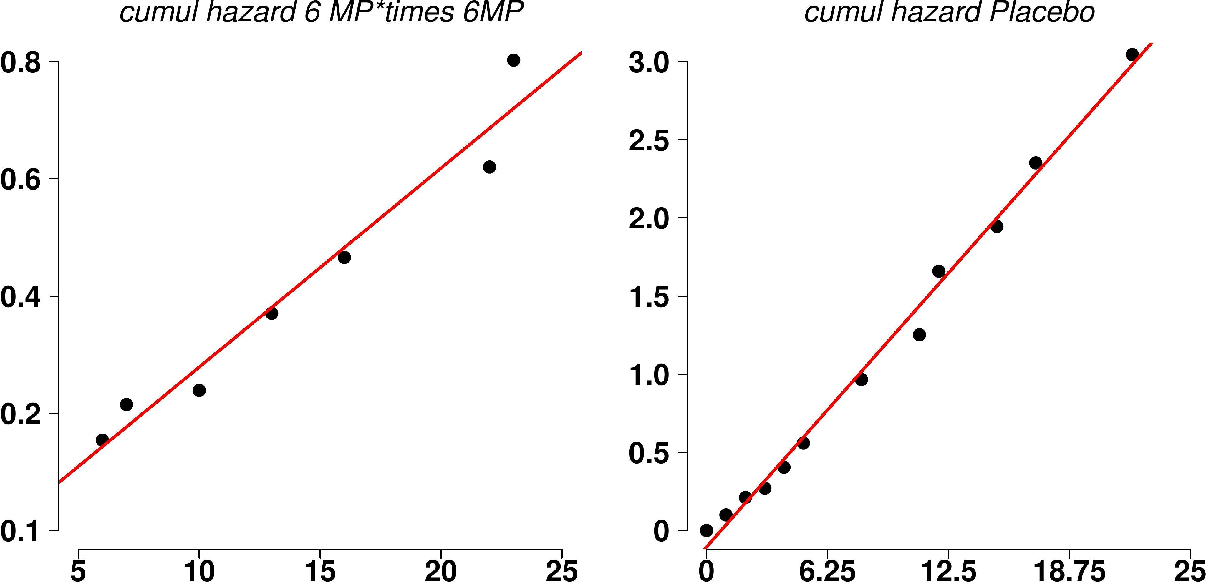
Cumulative hazards functions versus times for both treatment.

Empirical preliminary estimators for the parameter $\beta$ in the proportional hazards model $G(x)=x$ could be obtained from a preliminary data analysis using the Kaplan-Meier estimate of the survival function. From the Kaplan and Meier (1958) estimator for the survival function in each treatment, we could estimate the accumulated hazard function $\Lambda(t)=\int_{0}^{t}e^{\beta z}h(u)du=-\log[S(t,z)]$ , with $z=0$ for the 6MP treatment and $z=1$ for the placebo treatment. Table 1 shows the estimates of the cumulative hazard function based on the non-parametric Kaplan-Meier estimates for the survival function $S(t,z)$ for the treatment. Figure 1 shows the plots of the accumulated hazards functions $\Lambda(t)$ versus time for the two treatments, indicating good linear relationships.

Table 2

Kaplan-Meier survival function and accumulated hazard estimates

$t$	$\Lambda_{1}(t)$	$\Lambda_{2}(t)$	$\Lambda_{2}(t)/\Lambda_{1}(t)$	$\log(\Lambda_{2}(t)/\Lambda_{1}(t))$
1	$-$ 0.012	0.010	$-$ 0.820
2	0.021	0.152	7.249	1.981
3	0.054	0.294	5.421	1.690
4	0.088	0.437	4.982	1.606
5	0.121	0.579	4.785	1.566
6	0.154	0.721	4.674	1.542
7	0.188	0.863	4.602	1.526
8	0.221	1.006	4.551	1.515
9	0.254	1.148	4.514	1.507
10	0.288	1.290	4.486	1.501
11	0.321	1.432	4.463	1.496
12	0.354	1.574	4.445	1.492
13	0.388	1.717	4.429	1.488
14	0.421	1.859	4.417	1.485
15	0.454	2.001	4.406	1.483
16	0.487	2.143	4.396	1.481
17	0.521	2.285	4.388	1.479
18	0.554	2.428	4.381	1.478
19	0.587	2.570	4.374	1.476
20	0.621	2.712	4.369	1.474
21	0.654	2.854	4.363	1.473
22	0.687	2.996	4.359	1.472
23	0.721	3.139	4.355	1.471
24	0.754	3.281	4.351	1.470
25	0.787	3.423	4.347	1.470

From fitted standard linear regression models (least squares estimators) relating $\Lambda(t)$ and the survival times $t$ considering the data of the two treatments, we get the fitted simple linear regression models: $\widehat{\Lambda(t)}=-0.04563+0.0332t$ (6MP treatment) and $\widehat{\Lambda(t)}=-0.1321+0.1422t$ (placebo). Table 2 shows the predictions for the cumulative hazard functions $\lambda(t)$ assuming $t=1,2,\ldots,25$ for each treatment and for the ratio of the cumulative hazard functions $\Lambda_{2}(t)/\Lambda_{1}(t)$ which gives empirical estimates for $e^{\beta}$ in the proportional hazards model. Table 2 also shows the empirical estimates for $\beta$ given by $\log(\Lambda_{2}(t)/\Lambda_{1}(t))$ . The average of the empirical estimates for $\beta$ is given by $1.52591$ .

Assuming the Cox (1972) proportional hazards model, where $h(t;z)=h_{0}(t)e^{\beta z}$ with $z=0$ for the 6MP treatment and $z=1$ for the placebo treatment, and the partial likelihood function Eq. (3) we obtained the maximum likelihood estimator (MLE) for the regression parameter $\beta$ (use of the R software), given by, $\widehat{\beta}=$ 1.509 (0.470) where the value in parentheses is the standard error, an estimate close to the empirical estimate obtained using Kaplan Meier estimation method, indicating that the proportional hazards model is well fitted by the data. That is, the hazards ratio $h(t;z=1)/h(t;z=0)$ is given by $\exp(1.509)=4.52221$ , showing the efficacy of the drug 6MP to increase the remission times of the leucemia patients (greater risk for remission of the placebo patients).

Assuming a hierarchical Bayesian analysis of the proportional hazards model $(G(x)=x)$ the hazard function $d_{i}=h_{0}(t_{i})$ , $i=1,2,\cdots,n$ is assumed as an unknown latent random quantity with a specified probability distribution $\Lambda_{0}(t_{i})=d_{i}t_{i}$ , where $h_{0}(t_{i})=d\Lambda_{0}(t_{i})/dt_{i})$ . We assume in the first stage of the hierarchical Bayesian analysis, independent prior distributions $d_{i}\sim G(1,\tau_{\lambda})$ ; $\theta\sim G(45,10)$ where $\theta=\exp(\beta)$ and in the second stage of the hierarchical Bayesian analysis, we assume $\tau_{\lambda}\sim U(0,1000)$ . Observe that we are using some prior information in the choice of the prior distribution for the regression parameter $\beta$ , obtained from the use of the Kaplan-Meier estimator for the survival function (see Table 2) where the average of the empirical estimates for $\beta$ is given by, $1.52591$ or $\theta=e^{\beta}=4.59933$ , that is, we are using empirical Bayesian methods (Carlin & Louis, 2010). We are also using a very non-informative prior distribution for the unknown parameter $\tau_{\lambda}$ of the distribution for the latent variable $d_{i}$ . Using the OpenBUGS software (Spiegelhalter et al., 2003) considering a burn-in sample of 11,000 simulated samples discarded to eliminate the effects of the initial values in the iterative procedure and taking a final sample of size 1,000 (every 100 ${}^{\text{th}}$ in 100,000 generated Gibbs samples) to get the Monte Carlo Carlo estimates for the parameters of interest, the posterior mean for $\beta$ is given by 1.532 and standard deviation 0.1392 with a 95% credible interval given by (1.254, 1.809). Observe that the obtained Monte Carlo Bayesian estimate (posterior mean) is very close to the empirical estimate of (1.526) and very accurate since the estimate for the posterior standard deviation is given by 0.1392, much smaller than the standard deviation obtained using the partial Cox proportional hazards likelihood (0.470). The OpenBUGS code can be supplied upon request.

Assuming a non-informative prior for the parameter $\theta=e^{\beta}$ , $\theta\sim G(0.01,0.01)$ and the same simulation scheme used above with the OpenBUGS software, the posterior mean for $\beta$ is given by 1.946 and standard deviation (0.439) with a $95\%$ credible interval given by (0.0165, 2.691). From this result, we observe that the use of a more informative prior for the parameter $\theta$ using an empirical method to get some prior information is very important to get accurate inference results given the sensibility of the Bayesian results assuming different priors. Alternatively, we could use informative prior distributions for the regression parameters from prior information of medical experts.

4.2 Example 2

In this example, let us consider the data (survival times in days) from $35$ cancer patients treated at the Mayo Clinic (Fleming et al., 1980): data from sample 4.1 (large tumor): 28, 69, 175, 195, 309, 377 $+$ , 393 $+$ , 421 $+$ , 447 $+$ , 462, 709 $+$ , 744 $+$ , 770 $+$ , 1106 $+$ , 1206 $+$ ; data from sample 4.2 (small tumor): 34, 88, 137, 199, 280, 291, 299 $+$ , 300 $+$ , 309, 351, 358, 369, 369, 370, 375, 382, 392, 429 $+$ , 451, 1119 $+$ . Define the covariate $Z$ denoting both sample groups: $Z=1$ for large tumor and $Z=0$ for small tumor. Thus, we have the following expression for the hazard function that defines the Cox model: $h(t\mid x)=h_{0}(t)e^{\beta z}$ . In this way, when $z$ is equal to $1$ (large tumor), and $z$ is equal to $0$ (small tumor), we have: $h(t\mid z=1)=h_{0}(t)e^{\beta}$ if $z=1$ and $h(t\mid z=0)=h_{0}(t)$ if $z=0$ . The Cox proportional hazards model was fitted for tumor size (large and small tumors). It was found that there is a difference in survival time between the two groups. The large tumor group has the highest survival times. The MLE estimate for $e^{\beta}$ using the partial likelihood function Eq. (3) is given by 0.327 and the 95% confidence interval is given by (0.123; 0.865). The MLE estimate of the $\beta$ coefficient estimator is given by $-$ 1.119. This means that the probability of surviving the event is higher in the large tumor group, that is, the risk of failure is 67.3% lower in the large tumor group when compared to the small tumor group.

Considering a Bayesian approach with MCMC (Markov Chain Monte Carlo) methods, we assume in the first stage of the hierarchical Bayesian analysis independent prior distributions $d_{i}\sim G(1,\tau_{\lambda})$ and $\theta\sim G(3.26,10)$ (where $\theta=e^{\beta}$ ) using empirical Bayesian methods (use of some prior information in the choice of the prior distribution for the regression parameter $\beta$ , obtained from the use of the Kaplan-Meier estimator for the survival function)

In the second stage of the hierarchical Bayesian analysis, we assume $\tau_{\lambda}\sim U(0,1000)$ . Using the OpenBUGS software (Spiegelhalter et al., 1993) considering a burn-in sample of 11,000 simulated samples discarded to eliminate the effects of the initial values in the iterative procedure, and taking a final sample of size 1,000 (every 100 ${}^{\text{th}}$ in 100,000 generated Gibbs samples) to get the Monte Carlo Carlo estimates of interest, we get the posterior mean for $\beta$ given by $-$ 1.103 and standard deviation (0.1701) with a 95% credible interval given by ( $-$ 1.452, $-$ 0.7915).

Observe that the obtained Monte Carlo Bayesian estimate (posterior mean) given by $-$ 1.10 for the regression parameter $\beta$ is close to the maximum likelihood estimate of $\beta$ ( $-$ 1.12) using the partial likelihood function Eq. (3) and very accurate since the estimate for the posterior standard deviation is given by 0.1701.

4.3 Example 3

In this example, the data considered refer to a study described in Klein and Moeschberger (1997), carried out with 90 male patients diagnosed in the period 1970–1978 with laryngeal cancer and who were followed up to 01/01/1983. For each patient, age (in years) was recorded at diagnosis and the stage of the disease (I $=$ primary tumor, II $=$ involvement of nodules, III $=$ metastasis and IV $=$ combines the three previous stages) as well as their respective failure or censor times (in months). The stages are ordered by the degree of seriousness of the disease (less serious to more serious).

Assuming the Cox (1972) proportional hazards model where $h(t;z)=h_{0}(t)e^{\bm{\beta z}}$ with the covariate vector $\bm{z}=(z_{1},z_{2},z_{3},z_{4},z_{5},z_{6},z_{7})$ , $z_{1}$ denotes stage II, $z_{2}$ denotes stage III, $z_{3}$ denotes stage IV, $z_{4}$ denotes age, $z_{5}$ denotes the interaction between age and stage II, $z_{6}$ denotes the interaction between age and stage III and $z_{7}$ denotes the interaction between age and stage IV, and the partial likelihood function Eq. (3), we obtained the maximum likelihood estimator (MLE) for the vector of regression parameters $\bm{\beta}$ (use of the R software), given by, $\widehat{\beta_{1}}=$ $-$ 7.9461, $\widehat{\beta_{2}}=$ $-$ 0.1225, $\widehat{\beta_{3}}=$ 0.8470, $\widehat{\beta_{4}}=$ $-$ 0.0026, $\widehat{\beta_{5}}=$ 0.1203, $\widehat{\beta_{6}}=$ 0.0114 and $\widehat{\beta_{7}}=$ 0.0137.

Considering a Bayesian approach with MCMC (Markov Chain Monte Carlo), we assume in the first stage of the hierarchical Bayesian analysis, independent prior distributions given by $d_{i}\sim G(1,\tau_{\lambda})$ ; $\theta_{1}\sim G(354,1000000)$ , $\theta_{2}\sim G(885,1000),\theta_{3}\sim G(2332,1000)$ , $\theta_{4}\sim G(997,1000)$ , $\theta_{5}\sim G(1128,1000)$ , $\theta_{6}\sim G(1011,1000)$ and $\theta_{7}\sim G(1014,1000)$ , where $\theta_{j}=e^{\beta_{j}},j=1,2,\cdots,7$ using empirical Bayesian methods (from the use of the Kaplan-Meier estimator for the survival function in the same way as used in example given in Section 4.1).

Table 3
Posterior summaries of interest

	Mean	SD	Lower 95%	Upper 95%
$\beta_{1}$	$-$ 7.9460	0.0519	$-$ 8.0360	$-$ 7.8400
$\beta_{2}$	$-$ 0.1209	0.0340	$-$ 0.1871	$-$ 0.0525
$\beta_{3}$	0.8459	0.0213	0.8028	0.8864
$\beta_{4}$	0.0134	0.0157	$-$ 0.0177	0.0400
$\beta_{5}$	0.1175	0.0085	0.0986	0.1313
$\beta_{6}$	0.0159	0.0069	0.0024	0.0302
$\beta_{7}$	0.0162	0.0083	$-$ 0.0001	0.0332
$\tau_{\lambda}$	40.9600	43.9300	3.1700	163.700
$\theta_{1}$	0.0004	0.00002	0.0003	0.0004
$\theta_{2}$	0.8866	0.0302	0.8293	0.9489
$\theta_{3}$	2.331	0.0495	2.2320	2.4260
$\theta_{4}$	1.0140	0.0159	0.9824	1.0410
$\theta_{5}$	1.1250	0.0096	1.1040	1.1400
$\theta_{6}$	1.0160	0.0070	1.0020	1.0310
$\theta_{7}$	1.0160	0.0084	0.9999	1.0340

In the second stage of the hierarchical Bayesian analysis, we assume $\tau_{\lambda}\sim U(0,1000)$ . Using the OpenBUGS software (Spiegelhalter et al., 1993) considering a burn-in sample of 11,000 simulated samples discarded to eliminate the effects of the initial values in the iterative procedure and taking a final sample of size 1,000 (every 100 ${}^{\text{th}}$ in 100,000 generated Gibbs samples) we obtained the Monte Carlo estimators for the posterior means of each regression parameter $\beta_{j}$ , $j=$ 1,2,…,7 (Table 3).

The obtained Monte Carlo Bayesian estimates (posterior means) given, respectively by $-$ 7.946, $-$ 0.1209, 0.8459, 0.0134, 0.1175, 0.0159 and 0.0161, for the regression parameters $\beta_{1},\beta_{2},\beta_{3},\beta_{4},\beta_{5},\beta_{6}$ and $\beta_{7}$ , are close to the maximum likelihood estimates $\widehat{\beta_{1}}=$ $-$ 7.9461, $\widehat{\beta_{2}}=$ $-$ 0.1225, $\widehat{\beta_{3}}=$ 0.8470, $\widehat{\beta_{4}}=$ $-$ 0.0026, $\widehat{\beta_{5}}=$ 0.1203, $\widehat{\beta_{6}}=$ 0.0114 and $\widehat{\beta_{7}}=$ 0.0137 that were obtained using the partial likelihood function Eq. (3) and are very accurate since the estimates for the posterior standard deviations are very small..

5. A simulation study

In this section, we assume simulated samples from the Weibull distribution with probability density function (pdf) $f(t)=at^{a-1}e^{-(t/b)^{a}}/b^{a}$ , $t>0$ , survival function $S(t)=e^{-(t/b)^{a}}$ and hazard function $h(t)=f(t)/S(t)=at^{a-1}/b^{a}$ , $a$ is the shape parameter and $b$ is the scale parameter. Let us assume only one covariate $Z$ ( $Z=0$ for treatment $1$ or control and $Z=1$ for treatment $2$ ) and the proportional hazards model $h(t)=h(t)e^{\beta z}$ . For treatment 1 (control, $Z=$ 0) we have the hazard function $h_{1}(t)=at^{a-1}/(b_{1})^{a}$ and for treatment 2 ( $Z=$ 1), we have the hazard function $h_{2}(t)=at^{a-1}/(b_{2})^{a}$ , that is, we are assuming the same shape parameter $a$ , but different scale parameters $b_{1}$ and $b_{2}$ . That is, $h_{2}(t)=at^{a-1}/(b_{2})^{a}=(b_{1}/b_{2})^{a}at^{a-1}/(b_{1})^{a}=e^{\beta}% at^{a-1}/(b_{1})^{a}=e^{\beta}h_{1}(t)$ (proportional hazards), where $e^{\beta}=(b_{1}/b_{2})^{a}$ , or, $\beta=a\log(b_{1}/b_{2})$ . For a simulation study, we assume $a=$ 1.5, $b_{1}=$ 30, $b_{2}=$ 50, that is, $\beta=a\log(b_{1}/b_{2})=1.5\log(30/50)=$ $-$ 0.766238. Also, let us consider $n=$ 100. Table 4 shows the generated data (without censoring and with censoring).

Table 4
Simulated data ( $n=$ 100; $a=$ 1.5, $b_{1}=$ 30, $b_{2}=$ 50, $\beta=$ $-$ 0.766238)

Group 1 (without censoring)
2.9	52.7	21.6	18.8	20.2	65.3	43.1	44.5	20.4	48.2
	(l)	(s)	(l)	(m)		(m)	(m, l)	(l)	(s)
29.8	16.5	46.4	2.7	44.4	34.7	20.6	42.9	41.6	18.2
	(l)	(l)	(l)			(s,m,l)	(s)	(s, l)
31.2	1.2	7.2	17.9	47.6	5.1	44.7	24.1	7.7	34.0
			(m)	(l)	(l)	(m, l)
16.3	11.2	16.4	74.1	12.3	3.6	29.0	59.8	4.8	39.3
	(l)		(s)		(l)		(l)	(l)	(s)
10.2	1.2	28.7	9.2	56.2	16.5	16.4	37.4	26.1	2.9
(m, l)	(l)	(m)	(m)	(m, l)	(m, l)		(m)		(m)
Group 2 (without censoring)
38.4	71.4	14.0	59.9	29.9	25.4	21.7	49.8	24.9	80.9
	(m)	(l)	(l)	(l)			(l)
34.3	75.1	78.1	26.5	54.5	16.9	95.9	47.6	0.9	13.2
	(l)	(l)	(m)	(m)	(m)	(m)	(l)		(m)
56.1	76.2	17.2	23.7	67.9	41.9	103.7	15.6	31.5	14.6
			(l)			(l)	(l)		(l)
30.0	53.0	30.5	69.6	77.0	73.8	47.1	22.0	57.9	110.9
(l)		(m, l)	(m)	(l)		(l)	(l)		(m, l)
59.9	10.7	149.9	32.7	19.5	37.1	41.5	29.9	29.9	28.7
(m, l)	(s, m)			(l)	(m, l)	(l)		(m)	(m)
Type I censoring – observations $>$ 60 are censored in 60 $+$
All observations above (without censoring) but considering observations $>$ 60 as censored in 60.
Type I censoring – observations $>$ 50 are censored in 50 $+$
All observations above (without censoring) but considering observations $>$ 50 as censored in 50.

(s) – small proportion of 8 censored observations; (m) – moderate proportion of 27 censored observations; (l) – large proportion of 43 censored observations.

Under a Bayesian approach using MCMC (Markov Chain Monte Carlo) methods and the OpenBUGS software, we get the following results:

Weibull regression model (without censored data) with the scale parameters $b_{1}=e^{\beta_{0}}$ and $b_{2}=e^{\beta_{0}+\beta_{1}}$ that is $\beta=a\log(b_{1}/b_{2})$ . Priors: $a\sim G(1,1)\beta_{0}\sim N(0,100)$ and $\beta_{1}\sim N(0,1)$ . $G(c,d)$ denotes a gamma distribution with mean $c/d$ and variance $c/d^{2}$ . Use of OpenBUGS software (burn-in sample $=$ 1000; 1000 additional Gibbs samples (every 10th sample)). Posterior mean(SD): parameter $a$ : 1.458 (0.1118); parameter $b_{1}$ : 29.78 (2.983); parameter $b_{2}$ : 50.94 (5.016); $\beta$ : $-$ 0.783 (0.2063).

Semiparametric model (without censored data) with $\beta=\log(\theta)$ and priors $\theta\sim G(46,100)$ ; $\tau_{\lambda}\sim U(0.00011,1000)$ . Posterior mean(SD): $\beta$ : $-$ 0.7360 (0.1335); $\tau_{\lambda}$ : 19.39 (3.239) and $\theta$ : 0.4833 (0.06432).

Semiparametric model (with a small proportion of randomly censored – 8 censored observations) with $\beta=\log(\theta)$ and priors $\theta\sim G(46,100)$ ; $\tau_{\lambda}\sim U(0.00011,1000)$ . Posterior mean(SD): $\beta$ : $-$ 0.7394(0.1317); $\tau_{\lambda}$ : 20.94 (3.523) and $\theta$ : 0.4816 (0.06335).

Semiparametric model (with a moderate proportion of randomly censored – 27 censored observations) with $\beta=\log(\theta)$ and priors $\theta\sim G(46,100)$ ; $\tau_{\lambda}\sim U(0.00011,1000)$ . Posterior mean(SD): $\beta$ : $-$ 0.7517 (0.1317); $\tau_{\lambda}$ : 27.88 (5.156) and $\theta$ : 0.4757 (0.06257).

Semiparametric model (with a large proportion of randomly censored – 43 censored observations) with $\beta=\log(\theta)$ and priors $\theta\sim G(46,100)$ ; $\tau_{\lambda}\sim U(0.00011,1000)$ . Posterior mean(SD): $\beta$ : $-$ 0.7551 (0.1343); $\tau_{\lambda}$ : 38.11 (7.345) and $\theta$ : 0.4742 (0.06331).

Semiparametric model (type I censoring – observations $>$ 60 are censored in 60 $+$ with 13 censored observations) with $\beta=\log(\theta)$ and priors $\theta\sim G(46,100)$ ; $\tau_{\lambda}\sim U(0.00011,1000)$ . Posterior mean(SD): $\beta$ : $-$ 0.7731(0.1321); $\tau_{\lambda}$ : 20.83 (3.682) and $\theta$ : 0.4656 (0.0619).

Semiparametric model (type I censoring – observations $>$ 50 are censored in 50 $+$ with 24 censored observations) with $\beta=\log(\theta)$ and priors $\theta\sim G(46,100)$ ; $\tau_{\lambda}\sim U(0.00011,1000)$ . Posterior mean(SD): $\beta$ : $-$ 0.7892 (0.1358); $\tau_{\lambda}$ : 22.36 (4.015) and $\theta$ : 0.4584 (0.0624).

From these results, we observe that the proposed methodology is very robust to the presence of censored data (the obtained posterior summaries are very close considering the different scenarios).

6. Concluding remarks

From the results obtained in this study, we observed that the use of a hierarchical Bayesian procedure for the proportional hazards model considering the complete likelihood function obtained from semiparametric or transformation models can be a good alternative for the use of the partial likelihood function introduced by Cox (1972), leading, in general, to similar point estimates and better precision (smaller standard deviations). It is important to point out that the classical estimates (MLE) obtained from the partial likelihood function use asymptotic normality results, which in general depend on large sample sizes to obtain good accuracy. This result could be of interest to medical researchers since the family of proportional hazards models is the most commonly used methodology in the analysis of medical lifetime data in the presence of censoring and covariates when the assumption of proportional hazards is verified. In a future study, we will explore the use of hierarchical Bayesian methods to other choices of semiparametric models when the assumption of proportionality for the hazards functions is not supported by data, since the class of transformation models is very flexible, leading a wide range of possibilities for the lifetime data analysis as observed in recent studies presented in the literature.

Footnotes

Acknowledgments

The authors are very grateful for the suggestions of the editor and reviewers that led to a great improvement in the manuscript.

References

Bennett

(1983). Analysis of survival data by the proportional odds model. Statistics in Medicine, 2(2), 273-277.

Carlin

& Louis

(2010). Bayes and empirical Bayes methods for data analysis. Chapman & Hall/CRC, 2010, 440.

Chen

D.-G.

Peace

K. E.

Lio

& Wang

(2013). Approximating the baseline hazard function by Taylor series for interval-censored time-to-event data. Journal of Biopharmaceutical Statistics, 23(3), 695-708.

Chen

Jin

& Ying

(2002). Semiparametric analysis of transformation models with censored data. Biometrika, 89(3), 659-668.

Chen

Lin

& Zeng

(2012). Checking semiparametric transformation models with censored data. Biostatistics, 13(1), 18-31.

Chib

& Greenberg

(1995). Understanding the Metropolis-Hastings algorithm. The American Statistician, 49(4), 327-335.

Cox

& Oakes

(1984). Analysis of survival data. Chapman and Hall, New York.

Cox

D. R.

(1972). Regression models and life-tables. Journal of the Royal Statistical Society: Series B (Methodological), 34(2), 187-202.

Demarqui

F. N.

Mayrink

V. D.

& Ghosh

S. K.

(2019). An unified semiparametric approach to model lifetime data with crossing survival curves. arXiv preprint arXiv:1910.04475.

10.

Fleming

Parapia

Morgan

& Child

(1980). Increased urinary B2-microglobulin after cancer chemotherapy 1, 2. Cancer Treatment Reports, 64(4-5), 581-588.

11.

Freireich

A. L. G.

Freireich

E. J.

Gehan

Frei

III Schroeder

L. R.

Wolman

I. J.

Anbari

Burgert

E. O.

Mills

S. D.

Pinkel

, et al. (1963). The effect of 6-mercaptopurine on the duration of steroid-induced remissions in acute leukemia: A model for evaluation of other potentially useful therapy. Blood, 21(6), 699-716.

12.

Gao

Zeng

& Lin

D.-Y.

(2018). Semiparametric regression analysis of interval-censored data with informative dropout. Biometrics, 74(4), 1213-1222.

13.

Gelfand

A. E.

& Smith

A. F.

(1990). Sampling-based approaches to calculating marginal densities. Journal of the American Statistical Association, 85(410), 398-409.

14.

Gelman

Carlin

J. B.

Stern

H. S.

& Rubin

D. B.

(2004). Bayesian data analysis Chapman & Hall. CRC Texts in Statistical Science.

15.

Guo

& Zeng

(2014). An overview of semiparametric models in survival analysis. Journal of Statistical Planning and Inference, 151, 1-16.

16.

& Yi

G. Y.

(2020). Parametric and semiparametric estimation methods for survival data under a flexible class of models. Lifetime Data Analysis, 26(2), 369-388.

17.

Kalbfleisch

& Prentice

(2002). The statistical analysis of failure time data, 2002. Wiley Series.

18.

Kaplan

E. L.

& Meier

(1958). Nonparametric estimation from incomplete observations. Journal of the American Statistical Association, 53(282), 457-481.

19.

Klein

& Moeschberger

(1997). Survival analysis: Techniques for censored and truncated data. New York: Springer-Verlag.

20.

Lawless

(1982). Statistical models and methods for lifetime data. New York: Wiley.

21.

& Lee

M.-L. T.

(2021). Semiparametric model averaging prediction for lifetime data via hazards regression. Journal of the Royal Statistical Society: Series C (Applied Statistics).

22.

Lin

Wei

& Ying

(2001). Semiparametric transformation models for point processes. Journal of the American Statistical Association, 96(454), 620-628.

23.

Lin

D. Y.

Wei

L.-J.

Yang

& Ying

(2000). Semiparametric regression for the mean and rate functions of recurrent events. Journal of the Royal Statistical Society: Series B (Statistical Methodology), 62(4), 711-730.

24.

Lin

D. Y.

& Ying

(1994). Semiparametric analysis of the additive risk model. Biometrika, 81(1), 61-71.

25.

& Kosorok

M. R.

(2005). Penalized log-likelihood estimation for partly linear transformation models with current status data. The Annals of Statistics, 33(5), 2256-2290.

26.

Race

J. A.

& Pennell

M. L.

(2021). Semi-parametric survival analysis via Dirichlet process mixtures of the First Hitting Time model. Lifetime Data Analysis, 27(1), 177-194.

27.

Rossini

& Tsiatis

(1996). A semiparametric proportional odds regression model for the analysis of current status data. Journal of the American Statistical Association, 91(434), 713-721.

28.

Selingerova

Katina

& Horova

(2021). Comparison of parametric and semi-parametric survival regression models with kernel estimation. Journal of Statistical Computation and Simulation, 91(13), 2717-2739.

29.

Song

Davidian

& Tsiatis

A. A.

(2002). A semiparametric likelihood approach to joint modeling of longitudinal and time-to-event data. Biometrics, 58(4), 742-753.

30.

Song

& Wang

(2008). Semiparametric approaches for joint modeling of longitudinal and survival data with time-varying coefficients. Biometrics, 64(2), 557-566.

31.

Spiegelhalter

D. J.

Dawid

A. P.

Lauritzen

S. L.

& Cowell

R. G.

(1993). Bayesian analysis in expert systems. Statistical Science, 8, 219-247.

32.

Spiegelhalter

D. J.

Thomas

Best

& Lunn

(2003). WinBUGS version 1.4 user manual. MRC Biostatistics Unit, Cambridge. Available from: http://www.mrc-bsu.cam.ac.uk/bugs.

33.

Sun

& Sun

(2005). Semiparametric linear transformation models for current status data. Canadian Journal of Statistics, 33(1), 85-96.

34.

Yang

& Niu

X.-F.

(2021). Semi-parametric models for longitudinal data analysis. Journal of Finance and Economics, 9(3), 93-105.

35.

Yang

& Prentice

(2005). Semiparametric analysis of short-term and long-term hazard ratios with two-sample survival data. Biometrika, 92(1), 1-17.

36.

Zeng

& Cai

(2010). A semiparametric additive rate model for recurrent events with an informative terminal event. Biometrika, 97(3), 699-712.

37.

Zeng

& Lin

(2009). Semiparametric transformation models with random effects for joint analysis of recurrent and terminal events. Biometrics, 65(3), 746-752.

38.

Zeng

Lin

& Lin

(2008). Semiparametric transformation models with random effects for clustered failure time data. Statistica Sinica, 18(1), 355.

39.

Zeng

Mao

& Lin

(2016). Maximum likelihood estimation for semiparametric transformation models with interval-censored data. Biometrika, 103(2), 253-271.

40.

Zeng

Yin

& Ibrahim

J. G.

(2005). Inference for a class of transformed hazards models. Journal of the American Statistical Association, 100(471), 1000-1008.

41.

Zhou

& Sun

(2017). A sieve semiparametric maximum likelihood approach for regression analysis of bivariate interval-censored failure time data. Journal of the American Statistical Association, 112(518), 664-672.

Semiparametric transformation model:A hierarchical Bayesian approach

Abstract

Keywords

1. Introduction

Remark (some preliminary results)

4.1 Example 1

Table 1 Kaplan-Meier survival function and cumulative hazard estimates

4.3 Example 3

Table 3 Posterior summaries of interest

Table 4 Simulated data ( n = 100; a = 1.5, b 1 = 30, b 2 = 50, β = - 0.766238)

Footnotes

Acknowledgments

References

Table 1
Kaplan-Meier survival function and cumulative hazard estimates

Table 3
Posterior summaries of interest

Table 4
Simulated data ( $n=$ 100; $a=$ 1.5, $b_{1}=$ 30, $b_{2}=$ 50, $\beta=$ $-$ 0.766238)