The impact of PD-LGD correlation on bank capital adequacy in nongranular loan portfolio 1

Abstract

The Central Banks discuss bank recapitalization arrangements. Markup to capital is needed because the current Basel approach is insensitive to some risks. As the Basel Committee moves from comprehensive risk modelling towards a revised, simplified, standardised approach, where one-two triggers measure risk, banking regulators increase demand for a capital add-on to meet unaccounted risks. The paper suggests the add-on estimates for the joint effect of the concentration and PD-LGD correlation risks leaving other unaccounted ones out-of-scope. The previous studies estimated add-ons for each risk separately. We show their joint impact on capital can be higher up to 5.3 times than the sum of two taken apart. Then previous results do not provide sufficient capital for a bank. We obtain that Basel underestimates the joint risk in 1.9 times on average. We expect that our contribution will be useful at least but not last for specialised lending (e.g. real estate and project finance), where the joint effect of concentration and PD-LGD correlation risks is the most observable.

Keywords

Basel capital add-on concentration PD-LGD correlation

1. Introduction

On November 28–29 2016 (Santiago, Chile), the Central Bankers proposed to increase bank capital requirements. This offer came not least because the particular risks are neglected by current Basel approach being applied to capital calculation in 27 countries. Practitioners and academics point out concentration risk and risk caused by a correlation between probability of default (PD) and loss given default (LGD) among those risks that ignored.2 Concentration risk arises from having a significant share of exposure to a small group of homogeneous counterparties. PD-LGD correlation brings to fat tails of portfolio loss distribution. The more likely the borrower is not to pay back on its debt, the more likely the recovered amount is tiny. To cover an omitted risk, bank regulators implement multiplier to risk weights assigned to assets. It reduces capital underestimation.

The Basel framework does not take into account correlation between PD and LGD and concentration in the capital requirements explicitly. However, the previous works show the correlation of risk parameters and concentration risk for the banking system are significant. First, Witzany (2009), Hu and Perraudin (2002), Chava et al. (2011), Carey and Gordy (2003), Altman et al. (2005), Giese (2005) found that PD-LGD correlation can be in both corporate and retail portfolios and varies from 8 to 80%. Second, the Basel Committee admits 9 out of 13 G10 banking crises occurred due to concentration risk over 1978–2002 (BCBSWP13, 2004, p. Table 6). Acharya and Steffen (2015) show that banks enhance concentration by the sovereign debt to EU countries experiencing a severe economic downturn over 2011–2012. Tabak et al. (2011) found that Brazilian banks increase loan portfolio concentration gradually. Loutskina and Strahan (2011) note that US banks have the high concentration (4–18%) in mortgages until 2006. At last Enron and Worldcom are the most famous name concentration cases.

The PD-LGD correlation and concentration cause risks that are not covered by capital being evaluated using the current Basel approach. That is why the academics and practitioners estimated add-on to capital requirements to make Basel capital adequate. Meng (2010) and Miu and Ozdemir (2006) show that capital should be increased by 40% due to PD-LGD correlation. The BCBS Risk Concentration Group assessed the add-on for concentration should be 13–21%.3

We show that when two effects (concentration and PD-LGD correlation) present in a portfolio at the same time, their joint impact can be above the sum of effects taken separately. Therefore, the risk weight multipliers, defined for both effects independently in previous studies, can be inadequate to provide sufficient capital for a bank portfolio where two effects coincide.

The research objective is to verify that the capital adequacy estimation by the Basel approach is accurate and sufficient when both assumptions of the model (zero PD-LGD correlation and zero concentration risk) are violated at the same time. We also compare whether the current banking regulation initiative such as TLAC (total loss-absorbing capacity) is adequate to cover the joint effect.

We first estimate risk weight multiplier that considers the impact of two effects at the same time. We found that, on average, Basel underestimated the risk of correlation and concentration in 1.9 times. The joint effect of correlation and concentration required the capital in up to 5 times higher than the sum of both effects when the risks induce in portfolios separately. At the same time, we found that TLAC cover the losses of two effects in 61% portfolios among 640 examined.

The output is grounded not on mere logic, but also on rigorous analysis and vast data simulation. We analysed 640 unique hypothetical loan portfolios varied by risk level. Risk level is defined by the average portfolio PD, PD-LGD correlation, the concentration (Herfindahl-Hirschman Index). The risk parameters are generated from distributions confirmed in studies of the Basel Committee (bcbs256)4 and Standard & Poor’s research (Ozdemir & Miu, 2008). We estimated portfolio losses assuming that a loan is in default if its individual PD is higher than average one. We calculated capital for a portfolio by Basel approach (BCBS, Basel II, 2006, p. §272).5 The output of simulation was risk weight multiplier that is the portfolio losses over Basel capital. If the multiplier is more than 1, then Basel approach underestimates the losses, otherwise, overestimates. In order to ensure robust RW multiplier estimates we generate each unique portfolio 100 times. The final RW multiplier for the unique portfolio is the average of multipliers by each portfolio iteration. As a result, we have 64 000 observations.

The drawback of our research is that we estimate the losses from two effects, but cannot estimate the historical probability of its losses. In other words, there is no available data about how likely is the portfolio, where PD-LGD correlation and concentration exist together. Nevertheless, we observe increased attention to the problem of PD-LGD correlation for specialised lending (e.g. real estate and project finance) in revised standardised approach for credit risk published in December 2015 as consultation paper that most likely to be a part of Basel IV.6 Common counterparties can induce the concentration in project finance. Moreover, the concentration is discussed actively under the standards of internal capital adequacy process. Therefore, we suppose that the topic about the joint effect of PD-LGD correlation and concentration is actual.

The remainder of the paper is structured as follows. The second section provides an overview of the current Basel approach to credit risk estimation and its shortcomings. The result of previous research about PD-LGD correlation and concentrations are discussed in the section. Section 3.1 presents a theoretical example, where we show that the PD-LGD correlation and concentration create synergy effect (the joint effect is higher than a mere sum of two) when there is a positive correlation between exposure size and loss given default rate. Otherwise, there is a diversification effect, when PD-LGD correlation risk is compensated by the concentration of large loan with low loss rate. Sections 3.2–3.4 describe hypothesis, the methodology, and results of risk weight multipliers estimation. Sections 6 concludes.7

2. Related literature

2.1 Credit risk modelling in Basel II/III framework

2.1.1 Overview

Since 1974 the Basel Committee on Banking Supervision (hereafter – BCBS) has started to introduce the standards of banking regulation in response to the events in the banking systems (e.g. collapse of Herstatt Bank). The Committee aims at ensuring financial stability through the implementation of a unified set of standards for risk management.

Credit risk initially received increased attention from the BCBS as the primary risk for a bank. The Basel Committee released 611 documents with 20.5 thousand pages in all according to the website basel.io/analytics (as of May 2017). 21% of the documents (18% of total pages) was devoted to credit risk (Penikas, 2015). A publication on credit risk by the Basel Committee first appeared in 1982. Credit risk had been incorporated into all Basel frameworks, such as Basel I (1988), Basel II (2006), and Basel III (2010) standards. For comparison, operational and liquidity risks were considered only in Basel II and Basel III, respectively.

Basel requires a bank to hold sufficient capital to cover its risk if all borrowers occur in default. The capital should be at least 8% of bank risk-weighted assets (RWA) ((BCBS, Basel II, 2006, p. §40), (BCBS, Basel III, 2011, p. §131)). Basel II and Basel III offer banks to choose either the standardised approach or the approach based on internal models to calculate capital adequacy. The standardised approach defines RWA as the sum of assets weighted to its risk weight. BCBS fixes risk weights and ranged based on asset type and exposure’s external credit ratings or country risk scores of export credit agencies (ECA). The internal rating-based approach suggests calculating capital adequacy ratio (hereafter – CAR) using the Vasicek formula (Vasicek, 1987) (BCBS, Basel II, 2006, p. §272) (formula 2–4).

The Vasicek model applies credit risk parameters such as PD, LGD, EAD, and M, assessed by internal models, after these models are approved by the national regulator. Penikas (2015) shows internal credit risk assessment models first appeared in BCBS publication ‘bcbs49’ in April 1999. Banks can implement internal ratings-based (IRB) approach in basic (foundation IRB, F-IRB) and advanced (advanced IRB, A-IRB) version. Under the foundation IRB option, a bank computes only the probabilities of default (PD) of its borrowers; other factors are taken predetermined and constant as it is specified in the BCBS standards or by the national regulator. Under the advanced approach, a bank models loss given default (LGD), exposure at default (EAD) and maturity (M) in addition to the probability of default (PD) for every borrower. For example, a bank sets loss given default for all senior non-secured by recognized collateral at 45% using foundation IRB (BCBS, Basel II, 2006, p. §287), while the advanced IRB approach assumes LGD can take any value from 0% to 100% in accordance with the risk profile of the borrower based on bank’s internal models.

In July 2013 and in March 2016, BCBS published the documents (BCBS256, 2013) and (bcbs_d362, 2016), where expressed his lack of confidence in the credibility of internal bank models. First, internal statistical models provide more flexibility for risk assessment compared with a standardised approach. A bank can specify (manipulate) default definition, margins of conservatism in risk parameter estimates, adjustments for cyclical effects, the length of the data series used for estimation, etc. (please, see (BCBS256, 2013) for more details). Second, the low-default nature of asset classes, such as banks, large corporates with total assets exceeding 50bln euro, and small portfolio, such as specialised lending, provides unreliable statistical estimates due to insufficient data. Third, other asset classes, e.g. equities, requires more insights, than public data can cover, to assess credit risk faithfully.

Therefore, Basel IV framework, which is not yet approved but already being discussed (e.g. 28–29 November 2016, Chile), addresses the topics of reforming approaches to the credit risk assessment. BCBS wants to reduce risk-weighted assets variability among banks applying internal statistical models. The committee revises standardized approach to make it suitable alternative to internal models. BCBS proposes to classify exposures into buckets based on one or two triggers relevant to its asset type and to introduce the restrictions on the difference between RWAs based on IRB and standardized approaches (please, see capital floors in (bcbs_d306, 2015)).

However, the Basel Committee focuses on the inputs, while not paying sufficient attention to the methods. Today the BCBS does not solve the problem of capital adequacy underestimation caused by Vasicek model limitations.

2.2 The shortcomings of Basel II/III credit risk approach

In 1987 Oldrich Vasicek developed a distribution function of loan portfolio losses. Vasicek (1987) showed that if the number of loans in the portfolio tends to infinity, then for a given value of a single common latent Gaussian factor Y, describing the state of the economy, the share of defaulted loans converges to probability. Since 2004, when the Vasicek model was officially presented in Basel II framework, loan loss distribution became the basis for IRB capital calculation for 27 countries that adopted the Basel standards. According to reports, published by BCBS during Regulatory Compliance Assessment Programme (RCAP), more than 2,000 banks applied the Vasicek model for capital estimation.

The Eq. (2) is the basis for capital calculation under internal rating approach. However, the model has disadvantages that have been recognised by academic and banking community not less than 17 years ago. Among these disadvantages are the following.

1.
A macroeconomic state is described by a single common latent Gaussian factor, which is a simplification compared to reality (Pykhtin, 2004).
2.
The Vasicek model does not account for the correlation between probability of default and loss given default (Altman, 2001).
3.
It is assumed that a credit portfolio is adequately diversified (full granular), that is, there is no idiosyncratic risk (specific risk of the borrower) (Gordy & Lütkebohmert, 2013).
4.
Wrong assumption about asset correlation (R) (Khorasgani & Gupta, 2017);
5.
Wrong assumption about normally distributed probability of default;

Five issues above distort bank capital that can lead to its underestimation.

Further, our paper focuses on problems 2 and 3 in the list above.
2.3 Banking regulation response to low bank capital level

The regulators responded to the problem of low bank capitalisation. US banking regulators implement TLAC (total loss-absorbing capacity), while European regulators introduce MREL standards (own minimum funds and eligible liabilities).

TLAC defines a minimum requirement on the liabilities side for 30 global systemically important banks (G-SIBs).8 The G-SIBs should hold at least 16% (against current 8%) of consolidated risk-weighted assets (RWAs) and 6% of Basel III leverage ratio denominator from 1 January 2019. The requirements will become tougher since 1 January 2022, when banks are required to have capital equal 18% of consolidated RWAs and 6.75% of Basel III leverage ratio denominator.9

MREL is applicable for all EU banks. Add-on to capital is determined per bank.

TLAC and MREL options are used in the current research in the following way. We assess how strong the tightened requirements relative to Basel (in parallel with Basel standards) are adequate to cover the risk of PD-LGD correlation and concentration concurrently.

2.4 PD-LGD correlation

The Probability of default (PD) and loss given default (LGD) depend on company asset value that makes them dependent on each other. The stronger problems (economic environment, specific problem at microeconomic level) a company has, the higher the probability that the company will not be able to repay the debts. Strong problems often lead to intense asset write-down, thus reduces the assets which a bank may charge as a recovery. The latter one increases the losses of the bank given company’s default.

Figure 1 shows previous empirical findings of PD-LGD correlation estimated over different periods by eight papers. The higher line, the higher PD-LGD correlation was found. The length of the line shows the length of the observation period. The time series of the share of world income under banking crises allows concluding how PD-LGD correlation changes over an economic cycle. The more concentrated observation period near banking crises years, the higher PD-LGD correlation is.

Figure 1.

Empirical PD-LGD correlation estimates result over 2000–2014. Banking crises source: (Reinhart & Rogoff, 2009). URL: 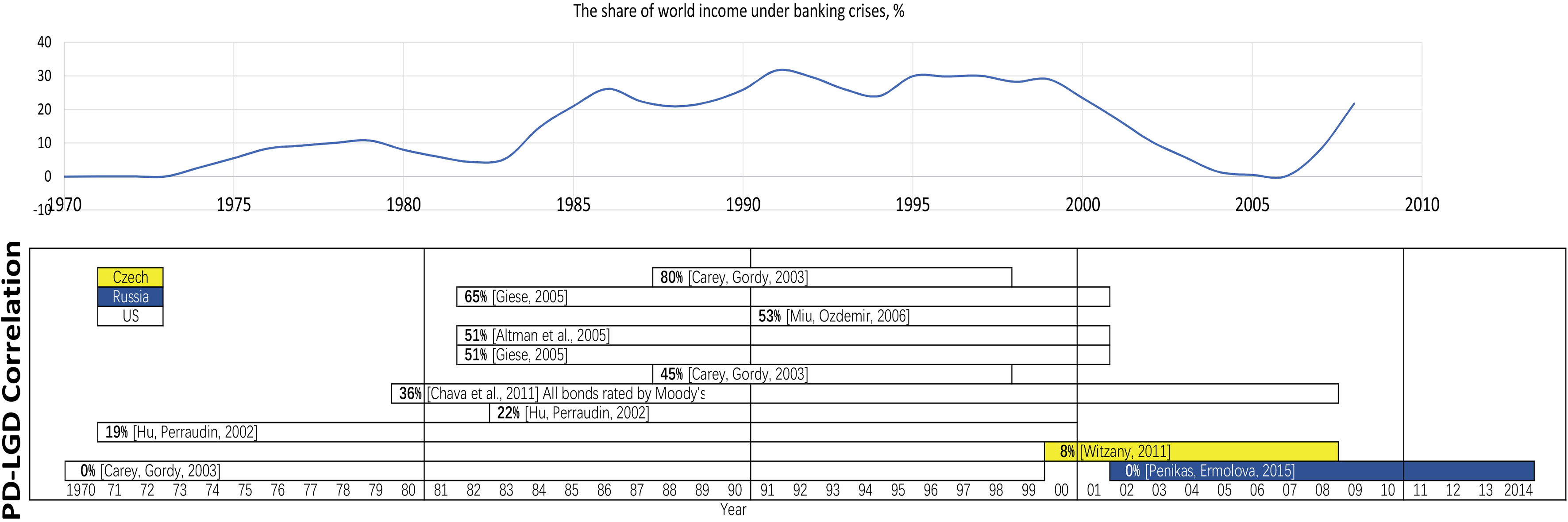http://www.carmenreinhart.com/user_uploads/data/205_data.xlsx.

Figure 1 presents that the most studies about PD-LGD relationship are based on US data. Only (Witzany, 2009) and (Ermolova & Penikas, 2017) study the dependence of PD and LGD using Czech and Russian data, respectively. US data is the most accessible because there is a Moody’s database with defaults (since 1920) and losses (since 1960). That is the reason why so far there have been no studies about PD-LGD correlation problem for Russia.

Further, the most recent research about PD-LGD correlation will be discussed.

Using 1,000 US senior unsecured bonds between 1982 and 2011 covered ten industry, Han (2016) found that PD-LGD dependency is equally well fitted to power ( $\text{LGD}_{i}=\varphi_{0i}\text{PD}_{i}^{\varphi_{1i}}$ ; R ${}^{2}=$ 0.56), linear ( $\text{LGD}_{i}=\varphi_{0i}+\varphi_{1i}\text{PD}_{i}$ ; R ${}^{2}=$ 0.54), and logistic ( $\text{LGD}_{i}=\frac{1}{1+\exp(-\varphi_{0i}-\varphi_{1i}\text{PD}_{i})}$ ; R ${}^{2}=$ 0.55) functions regarding R-square. The main significant difference between the functional forms is their impact on expected and unexpected losses. Expected losses are the largest for the power function because the power function gives the highest value of LGD (58%) at the point of 1.67%, which corresponds to the average PD for US bonds over 1982–2011. At the same time, LGD increment reduces with increasing PD under power model. Therefore, a larger value gets the LGD obtained via the linear model for PD above 3.5%. Han (2016) concluded that the linear model produces the highest risk in the tails. Consequently, unexpected losses are the largest under linear model for the high confidence level.

The research of (Eckert et al., 2016) extends (Miu & Ozdemir, 2006) by introducing the dependency of PD and LGD with the third key parameter EAD (exposure at default) involved in the credit risk estimation. First (Eckert et al., 2016), specify the Heckman’s model for loss estimation. Selection equation specifies default event (1 if default; 0, otherwise). Three regression equations describe utilisation rate at default (URD), secured and unsecured recovery rates (SRR, URR). URD defines exposures at default, while loss given default is introduced through SRR and URR. If a hypothesis of non-zero regression parameter lambda in the Heckman model is not rejected, then PD, LGD, and EAD are dependent. Second, Eckert et al. (2016) show that a bank needs to increase its capital by 1.93 times to consider PD-LGD-EAD correlation equal to 0.7.

Fischer et al. (2016) incorporate PD-LGD dependence into widespread CreditRisk $+$ model produced by Credit Suisse Group in 1996. CreditRisk $+$ does not analyse a reason for default but assume default rate as random process with a given intensity. PD-LGD correlation is introduced by Gamma-distributed specific sector and common background factors that define both the intensity of default and loss given default. Common background factors make sectors to be dependent. Using benchmark portfolio, suggested by International Association of Credit Portfolio Management (IACPM) and International Swaps and Derivatives Association (ISDA) in 2006, the authors show that expected losses and Value-At-Risk at 99% increase by 7% and 24%, respectively, with increasing PD-LGD by 0.1.

Cohen and Costanzino (2017) notice that the economic capital models are more adapted to a stochastic recovery than asset pricing models, where it still assumes deterministic recovery. The practice of stochastic recovery is used in the pricing models of Collateralized Debt Obligations (CDO) rather than bonds and Credit Default Swaps (CDS). Cohen and Costanzino (2017) show that the Merton asset pricing model defines stochastic recovery equal to the difference between stochastic assets and constant liabilities at the maturity. However, Black and Cox (1976) allows a default to happen before maturity in the Merton model, recovery becomes constant because default occurs when asset equals predetermined liabilities (Cohen & Costanzino, 2017).

2.5 Concentration risk

Granularity adjustment is the most popular treatment for concentration discussed by academics. Gordy and Marrone (2012) define a fine-grained portfolio as a portfolio with sufficiently diversified idiosyncratic risk where the weight of each loan in the portfolio achieves at zero. If the portfolio is granular, then its risk almost entirely depends on systematic risk. Gordy and Marrone (2012) represent this statement as the equality of qth quantile of simple average portfolio loss rate and qth quantile of expected loss rate conditioned on a systematic factor. If a portfolio is not fine-grained, then the equality does not hold. Gordy and Marrone (2012) define granularity adjustment as the difference between those two quantiles. In other words, the granularity adjustment should be found such that to cover the effect of undiversified risk in the portfolio. The analytical form of granularity adjustment has obtained by Taylor expansion.

Gordy and Lütkebohmert (2013) fit the adjustment for Basel II approach using Credit Risk $+$ framework. The adjustment is presented in simplified and comprehensive forms. The losses are defined using standard bank inputs (PD, LGD, EAD) and regulatory parameters (quantile level, systematic risk distribution parameters).

The history of granularity adjustment dates from 2003 when Gordy (2004) firstly introduced the method to cover concentration risk. Hibbeln (2010, p. 70) noted that the adjustment was published in the second Consultative Paper of Basel II but not included in the final standards. The Basel Committee points out that the approach is used mostly by large banks because its accuracy decreases for portfolios less than 200 obligors of low quality or 500 obligors of investment-grade quality (BCBSWP15, 2006).

The Russian banking regulation does not implement concentration into economic capital model explicitly. The Central Bank of Russia restricts the share of large loans by the regulatory ratio N7 (CBR Regulation No. 139-I). The maximum loan minus reserves have to be no more than 850% of capital. Additionally, a bank can introduce its internal limit in compliance with risk appetite.

The BCBS Concentration Risk Group of the Research Task Force concludes the value at risk increases by 13 to 21% (BCBSWP15, 2006). Gordy and Lütkebohmert (2006) assess 4 and 8% value-at-risk rise for small portfolios (1 000 – 4 000 loans) and 1.5% to 4% for large ones (cit. by (BCBSWP15, 2006)).

Conversely, Jahn et al. (2013) argue that a bank boosts concentration if a bank has complete information, or can identify borrower’s type accurately. The authors use German banks’ loan information over 2003–2011. They show that concentrated banks have less unexpected credit risk, as the standard deviation of their loss rates is lower. Therefore, it is empirical cases when concentrated portfolio requires less capital than fine-grained.

2.6 Paper contribution

This paper contributes to the literature in the following ways. Despite the fact, some papers study the impact of PD-LGD correlation and concentration of loan portfolio on bank capital adequacy, the following unsolved questions leave. First, the works do not specify the impact on credit risk capital, if both effects are present in loan portfolio simultaneously. There is a need to study the interaction effect of both assumptions because the joint impact of two effects can differ from a mere sum of the two (see example in the next section). Therefore, a capital add-on for the joint effect should be defined.

3. Simulation study: The joint effect of PD-LGD correlation and exposure concentration

3.1 The joint effect is not a mere of the sum two

Consider 2 loans with the same exposure of 1$ each. There are four possible outcomes (the letters A, B, C, D on Figs 2 and 3). The portfolio loss is equal to zero, if both loans are paid (letter A). The portfolio loss is equal to 0.5$ or 0.8$ if the first loan (letter B) or the second loan (letter C) is in default, respectively. The maximum portfolio loss will be 1.3$ when both loans (letter D) default.

Figures 2 and 3 show loss distribution changes after adding PD-LGD correlation and exposure concentration for both positive and negative LGD-EAD correlation. The letters help to trace the points movement as correlation and concentration were added. LGD – loss given default, EAD – exposure at default.

Figure 2.

PD-LGD correlation effect.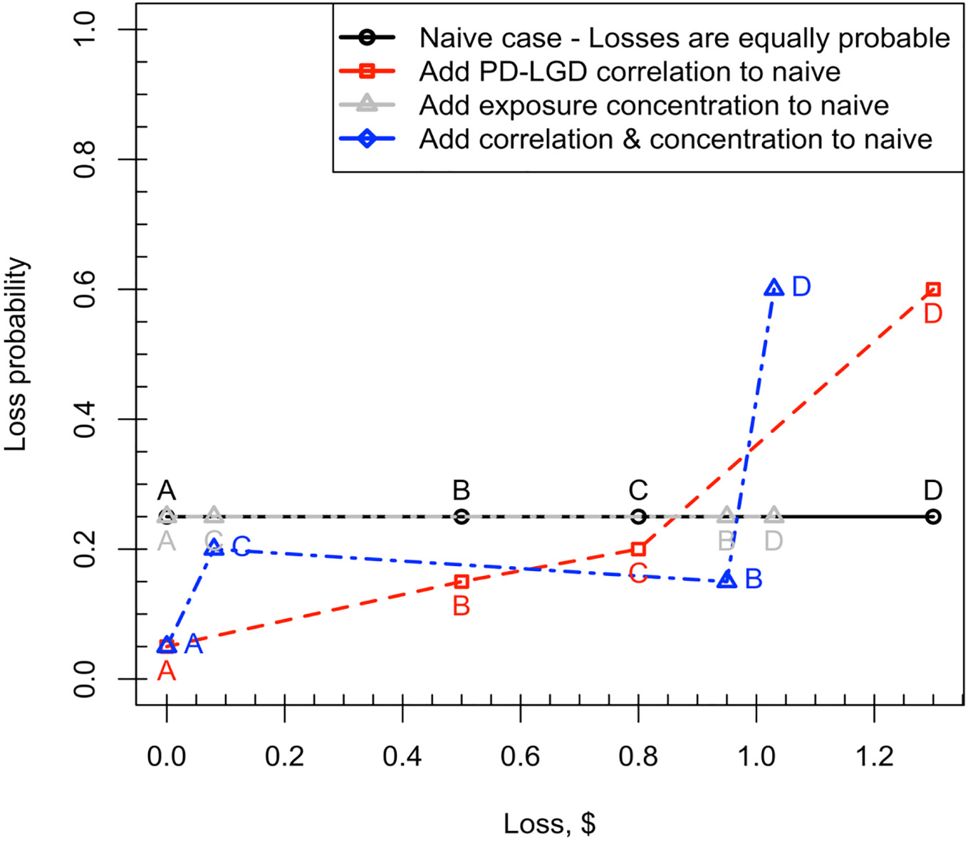

Figure 3.

PD-LGD correlation and exposure concentration effect.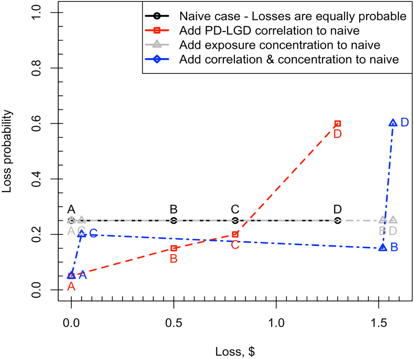

Start with the naïve case when four outcomes are equally probable (25%) (solid dark line). First, add PD-LGD correlation to the naïve case, i.e. the higher losses have higher probabilities (dashed red line). Now the distribution has heavy tails.

Return to the naïve case. Remain 25% as the probability of each possible outcome, but change the loans weights in portfolio making it concentrated. The loan sizes became 1.9$ and 0.1$ (total portfolio assets remain 2$). Here it makes sense to consider two cases (Figs 2 and 3 correspond to two cases). The first case assumes the positive correlation between loss given default (LGD) and exposure at default (EAD). The latter means that the higher exposure, the higher the loss rate. It can be a small company that borrows a large loan but is unable to pay a loan in default that leads to significant losses for the bank (e.g. Snapchat). The second case is the opposite, i.e. LGD-EAD correlation is negative. Imagine a rare default of large borrower (the Basel assume it occurs one time in 1000 years, see N (0.999) in Vasicek model). New loss distribution narrows when the LGD-EAD correlation is negative after adding concentration (dot-dash grey line) and expanded for positive LGD-EAD correlation case.

One can observe the significant difference in the case of two loans are in default (letter D) when two effects are added at the same time (dot-dash blue line). Negative LGD-EAD effect reduces losses compared with naïve case and PD-LGD correlation case, otherwise, with positive LGD-EAD dependency. The PD-LGD correlation increases the weight of problem loans in portfolio expected losses; the concentration can either increase or decrease the value of portfolio loss.

The sum of two effects taken separately differs from the joint effect. The negative LGD-EAD correlation strengthens risk, while positive one reduces portfolio risk.

We can conclude the following. If two problems are present in a portfolio, one cannot apply the multipliers to risk weight estimated in academic literature and by regulators in isolated cases. The PD-LGD correlation problem should be studied taking into account portfolio concentration.

3.2 Hypothesis

The theoretical example shows that the risk caused by both PD-LGD correlation and concentration can extend. Thus, we call into the question the adequacy of capital required by Basel.

Hypothesis: Basel underestimates losses caused the joint effect of PD-LGD correlation and concentration.

The hypothesis is not rejected if the capital requirement $K_{i}$ is less than the unexpected losses $L_{i}$ in each of the four cases.

Previous studies (see Fig. 1) refuted the Basel Committee’s evidence about the zero PD-LGD correlation, thus proving that the actual risk is above the risk assessment by the Basel II/III method. We declare that the risk may be disproportionately higher if the PD-LGD correlation is combined with the concentration risk. In this case, there are two options. If the concentration is observed for less risky borrowers (a negative relationship between loss rate and exposure), the effect of diversification is possible; otherwise, there is the synergy effect (disproportional increase in risk). It was shown in Figs 2 and 3.

4. Methodology

4.1 Generation of 640 of unique hypothetical portfolios

To generate hypothetical portfolios means to generate PD, LGD, EAD for all borrowers in the portfolio. The final hypothetical portfolio contained 100 unique borrowers. Such size of the portfolio can be weight with one used in BCBS research (bcbs256). One hundred of borrowers are compatible with the size of the corporate portfolio of an average Russian bank. We associate our portfolio with a portfolio of corporate borrowers because the concentration by the size of the credit claim is more proper to the corporate than to the retail portfolio due to the relatively smaller size of the number of corporate borrowers compared to retail borrowers. The PD-LGD effect is not associated with the type of portfolio and can be present in both retail (Witzany, 2009) and corporate portfolios (all other PD-LGD correlation research discussed in Section 2).

Further, PD, LGD, EAD is generated for each borrower. In reality, the Bank evaluates these parameters based on the characteristics of borrowers and the characteristics of the credit claim. We will generate random values which have distributions similar to those observed. The characteristics of the distribution are taken from the Basel Committee studies and (Ozdemir & Miu, 2008). Details are described below.

The probability of default is described by the normal truncated distribution in the range from 0 to 1 (Fig. 4). Appendix 3 of the document bcbs256 illustrates that the average PD value for the corporate portfolio is 5%. Five and 95 percentiles correspond to 1% and 17.5%, properly. The values are defined on 86 portfolios of 54 large international banks; the data was collected by the Committee’s Capital Monitoring Group. As can be seen from the above, we were considering four mean PD values: 1%, 5%, 10%, 20%. The standard deviation is intended to be about 3 percentage points.

Figure 4.

Distribution of default probability (PD).

Figure 5.

Distribution of loss given default (LGD).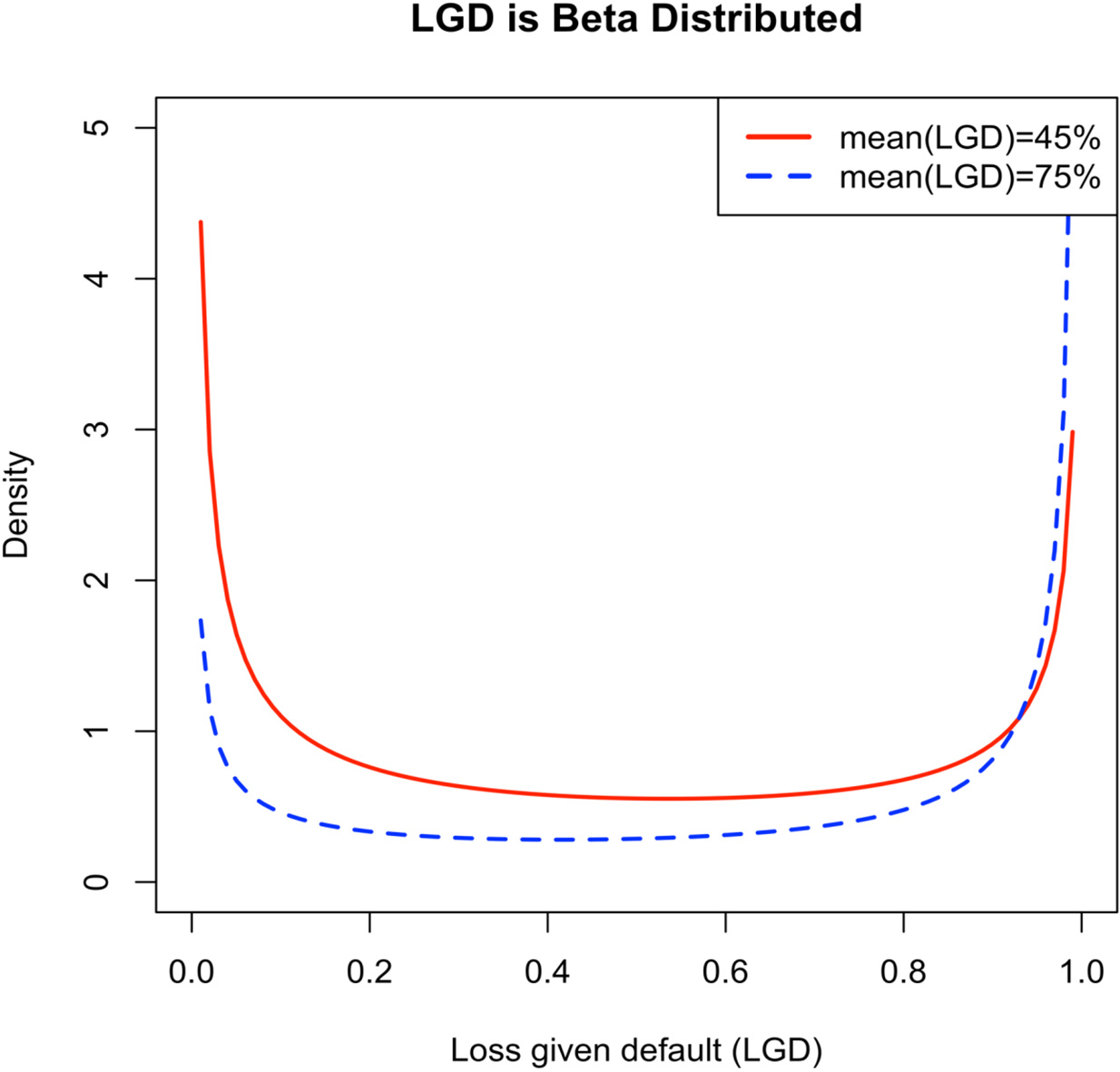

LGD is described by the beta distribution and has a U-shape (Fig. 5). The U-shape of the beta distribution is achieved if the distribution parameters a and b are less than one simultaneously. Parameters of a and b can be calculated by the average and variance distribution. The results of the bcbs256 research show that the average of LGD is 35%. Five and 95 percentiles correspond to 18.3% and 45.3%, properly. Nevertheless, here we are operating more with the Basel 2 values, which define LGD as 45% for senior uncovered credit claims. The standard deviation was compared to which was proposed in the research (Ozdemir & Miu, 2008). The U-shaped LGD distribution was proved in (Ozdemir & Miu, 2008) empirically.

Further, 5 PD-LGD correlation values are considered: {0%; 20%; 40%; 60%; 80%}. In previous studies, researchers received only a zero or positive PD-LGD correlation.

A multidimensional distribution of PD and LGD is set up in such a way that the given correlation is observed. The algorithm is implemented in R.10 The essence of the algorithm is as follows. The cumulative distribution of PD and LGD is set up separately. Further, the cumulative probabilities of each PD and LGD are put in correspondence to achieve a given correlation.

We obtain the multivariate distribution, which gives us to generate random PD and LGD.

EAD is modelled as follows. We hypothesise that the total portfolio exposure is 1000$ (that is, an average of $10 per borrower). The borrower will be assigned to EAD, depending on the given level of Herfindahl-Hirschman index.

The Herfindahl-Hirschman index is determined by the formula:

$\displaystyle\text{HHI}=\sum\limits_{i=1}^{100}\left(\frac{\text{EAD}_{i}}{% \sum\limits_{i=1}^{100}{\text{EAD}_{i}}}\right)^{2}$ (1)

We vary the Herfindahl Hirschman index from 0% to 18% (the index determination range is from 0% to 100%). We apply multipliers to increase the weight of large loans. A portfolio with greater correlation is rare in practice.

We also generate LGD-EAD correlation using multivariate distribution. We vary LGD-EAD correlation from 0% to 60% in increments of 20 percentage points.

The result is 640 loan portfolios with different risk level (4 PD * 5 PLC * 4 LEC * 8 HHI $=$ 640).11

4.2 The risk-weight multiplier estimation

The result of the simulation is risk-weight multipliers for all 64 000 portfolios. RW multipliers provide a sufficient level of capital to cover unexpected risks (the expected risks are covered with pricing). The multiplier is determined by the formula:

$\displaystyle\text{RW-mult}=\text{Model unexpected loss}/\text{Capital by Basel}$

As a result, within the framework of the simulation, it is important to obtain two components-portfolio losses and Basel capital.

4.3 Portfolio losses

After the portfolio is generated (PD, LGD, EAD are determined), default flag (binary indicator: $D_{i}=\{0,1\}$ ) is assigned for each loan in portfolio. We assume that the internal bank risk models provide accurate estimates of PDs such that the forecast values are equal to the realised ones, i.e. an average portfolio PD equals to portfolio default rate. Then the number of defaults in a portfolio should be equal $d=\text{PD}*n$ , where PD is the average portfolio PD and $n$ is the number of loans in the portfolio. Default is assigned to $d$ loans with the highest PDs.

The definition of default, given in Section 3.3, is applied for loans. The actual losses are the losses on default loans ( $\sum_{i=1}^{N_{d}}{\text{LGD}_{i}*\text{EAD}_{i}}$ , where $N_{d}$ – the number of default loans). Unexpected losses are the difference between actual losses on default loans and expected losses ( $\sum_{i=1}^{N}{\text{PD}_{i}*\text{LGD}_{i}*\text{EAD}_{i}}$ , where $N$ – the number of loans in a portfolio).

4.4 Capital

Capital is determined from the Vasicek formula according to paragraph 272 in Basel 2. We assume the 2.5 years term of the loan for all loans. All other parameters PD, LGD, EAD are known to us from the step where the portfolios were generated.

$\displaystyle\text{K}=\text{LGD}\left[\text{N}\left(\frac{\text{G}\left(\text{% PD}\right)+\text{G}\left({0.999}\right)*\sqrt{\text{R}}}{\sqrt{1-\text{R}}}% \right)-\text{PD}\right]*\frac{1+\left(\text{M}-2.5\right)\text{b}}{1-1.5\text% {b}}$ (2) $\displaystyle\text{R}=\frac{0.12\times\left(1-\exp\left(-50\times\text{PD}% \right)\right)}{{1-\exp(-50\times\text{PD})}}+\frac{0.24\times(1-\left(1-\exp% \left(-50\times\text{PD}\right)\right))}{1-\exp(-50\times\text{PD})}$ (3) $\displaystyle\text{b}=\left(0.11852-0.05478\times\ln\left(\text{PD}\right)% \right)^{{2}}$ (4)

Figure 6.

CySEC approach for concentration. Source: Cyprus Securities and Exchange Commission (hereafter – CySEC).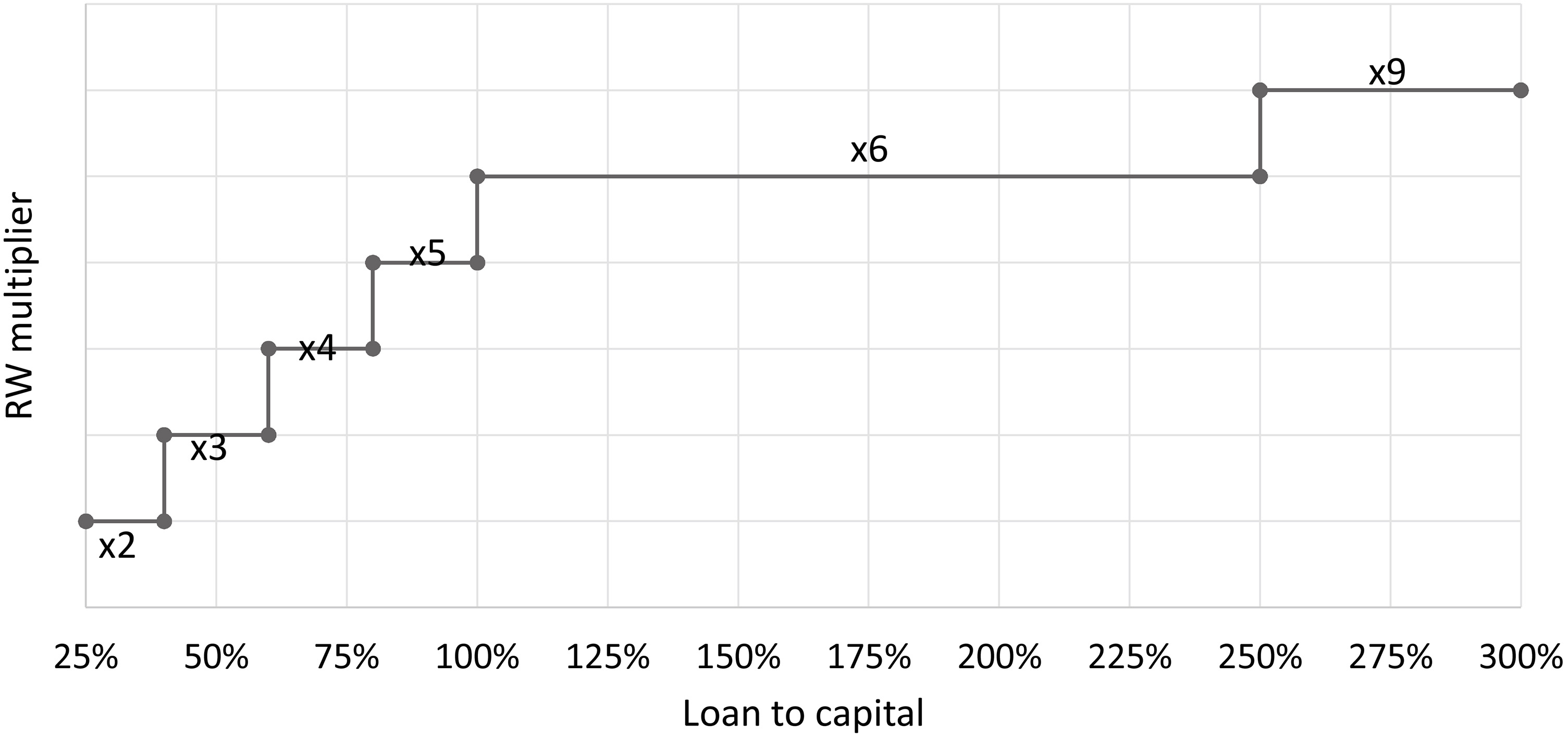

Assume M (maturity) equals 2.5 in compliance with Basel II standards; b $=$ maturity adjustment; R $=$ assets’ correlation. N (x) is the cumulative distribution function (CDF) of a standard normal random variable, G (z) is the inverse one.

The capital is calculated by two methods proposed by the Basel II. The first method (Foundation IRB, F-IRB, par. 246 Basel II) suggests that a bank applies constant LGD $=$ 45% for all loans, where 45% is the best estimate of LGD for corporate exposure, according to the Basel standards. The second method (Advanced IRB, A-IRB, par. 247 Basel II) proposes to evaluate LGD, i.e. to take into account the PD-LGD correlation. It turns out that in the first case, PLC is excluded from the capital calculation, because an increase in PD does not change LGD. In the second case, the correlation is taken into account.

Further, the obtained values of simulated unexpected losses and capital are compared, the weight risk multiplier. If the multiplier is more than 1, then Basel’s approach underestimates the losses, otherwise, overestimates.

4.5 Comparison with other concentration margin approaches

4.5.1 Cyprus approach

Cyprus regulators assign a concentration margin to credit requirements for which the ratio of transaction size to the capital exceeds the established threshold amounts (Fig. 6).

For example, if the transaction makes 85% of the capital, then the loan requirement, calculated with the Vasicek model according to the Eq. (2), is increased fivefold. The procedure is performed for each credit claim. The resulting multiplier of the risk weight is defined as the ratio of the amount of portfolio loan claims after applying the charge to the number of loan claims on the portfolio before applying the charge.

4.5.2 Slovenian approach

In the Slovenian approach, the capital requirement for the portfolio increases depending on the Herfindahl-Hirschman level for the 100 largest borrowers in the portfolio. The final multiplier is determined from the Table 1.

Table 1
Slovenian approach for concentration

Source: URL: www.bsi.si/library/includes/datoteka.asp?DatotekaId=4510.
Individual concentration index	Mark-up
$0<\textit{HHI}_{I}\leqslant 1$	0%
$1<\textit{HHI}_{I}\leqslant 2$	2%
$2<\textit{HHI}_{I}\leqslant 4$	4%
$4<\textit{HHI}_{I}\leqslant 10$	6%
$10<\textit{HHI}_{I}\leqslant 100$	8%

4.6 The simulation output

Finally, three types of RW multipliers are obtained:

1.
RW multiplier (capital add-on) as the result of our modelling (the excess of the simulated unexpected losses over the capital requirement according to the Vasicek formula)
2.
RW multiplier (capital add-on) based on Cyprus approach
3.
RW multiplier (capital add-on) based on Slovenian approach

5. Results

5.1 Capital add-on for PLC (PD-LGD correlation)

Suppose, there are granular (without exposure concentration) portfolios, consisting of 100 loans, where the exposure of each loan is 10$. The portfolios differ in the average probability of default (PD $=$ 1%, 5%, 10%, 20%) and PD-LGD correlation level (0%, 20%, 40%, 60%, 80%). The average LGD is 45% for each portfolio. We will estimate whether unexpected losses are covered by the capital calculated for these portfolios according to the Basel approach. The paper provides the results partially, for a portfolio with PD $=$ 5% and 20%, in particularly. The other results are available upon the request.

The Fig. 7 below shows the following evidence for mid-default portfolios. The average PD of portfolios equal to 5%. First, the capital by F-IRB approach is less than by A-IRB. Therefore, if there is the PD-LGD correlation in a loan portfolio, and the capital is calculated by F-IRB (constant LGD), it should be adjusted up to 14% (PLC $=$ 80%) depending on the level of correlation. On the other hand, under both foundation and advanced approaches, Basel capital covers unexpected losses by almost four times as a minimum. It means that the RW multiplier for the PD-LGD correlation is not required.

Figure 7.

Net impact of PLC on capital (portfolio PD $=$ 5%).

In contrast to the previous case, when the correlation increases from 20% to 80%, the ratio of capital to unexpected losses for high-default portfolio significantly decreases from 12 to 1.7 times. However, the capital calculated using Basel approach is still higher than unexpected losses.

Thus, we conclude that the PD-LGD correlation does not require any capital in addition to the Basel capital. It is true if bank’s internal models assess the risk of the loan portfolio accurately.

5.2 Capital add-on for exposure concentration

Further, examine a loan portfolio where PD-LGD correlation does not exist, but there is a concentration of loan exposure. The concentration is measured by the Herfindahl-Hirschman index. Next, we compare the unexpected losses and capital by Basel A-IRB approach.

In contrast to the PLC case, the risk of concentration is less incorporated into the Basel capital (Fig. 8). For the portfolio with average PD $=$ 20%, the capital is not sufficient to cover unexpected losses at HHI above 5%. The riskier the portfolio, the lower critical level of concentration is required for the positive capital add-on.

Figure 8.

Net impact of exposure concentration on capital (portfolio PD $=$ 20%).

5.3 The joint capital add-on for PLC and exposure concentration

One can conclude that the estimates of the net impact of PLC and exposure concentration are enough to calculate capital add-on for a portfolio where both peculiarities exist. The joint capital add-on can be equal to the sum of the two markups. Moreover, since we have received that no capital adjustment is required for PLC, the joint surcharge will be similar to the add-on for the concentration. Further, we test this hypothesis.

Take a portfolio where PD-LGD correlation and concentration of credit requirements are present simultaneously. Repeat calculations of unexpected losses and capital by F-IRB method (method with constant LGD) and compare them. The Table 2 shows how many times the capital should be increased to cover unexpected losses expanded by PLC and concentration. The Table 2 shows that the joint effect of correlation and concentration exceeds the sum of two net effects. For example, the concentration markup for PLC $=$ 60% is higher than for PLC $=$ 20%, despite the fact that PLC itself does not require the capital rise. It means that PLC boosts the effect of concentration. The higher the average portfolio probability of default, the higher the joint effect of correlation and concentration on losses and capital.

Table 2
The joint capital add-on for PLC and exposure concentration

Portfolio characteristics	HHI								Average RW
(average LGD $=$ 45%)	0%	1%	5%	10%	12%	14%	16%	18%	multiplier
Average PD $=$ 5%	1.0		1.4	2.1	2.3	2.5	2.6	2.7	2.1
PLC $=$ 0%			1.0	1.2	1.3	1.4	1.5	1.5	1.3
PLC $=$ 20%			1.1	1.7	1.9	2.1	2.2	2.3	1.8
PLC $=$ 40%	1.0		1.4	2.2	2.4	2.6	2.7	2.8	2.2
PLC $=$ 60%			1.6	2.5	2.7	2.9	3.1	3.2	2.4
PLC $=$ 80%			1.9	2.9	3.2	3.5	3.7	3.8	2.9
Average PD $=$ 20%	1.0	1.1	2.3	3.0	3.1	3.3	3.4	3.5	2.8
PLC $=$ 0%			1.2	1.4	1.4	1.4	1.4	1.4	1.3
PLC $=$ 20%	1.0		1.8	2.2	2.3	2.4	2.5	2.6	2.1
PLC $=$ 40%			2.4	3.1	3.2	3.4	3.5	3.5	2.9
PLC $=$ 60%	1.0	1.2	2.9	3.8	4.0	4.3	4.5	4.7	3.6
PLC $=$ 80%	1.0	1.5	3.4	4.4	4.6	4.9	5.1	5.2	4.1
Average RW multiplier	1.0	1.0	1.6	2.2	2.3	2.5	2.6	2.7	2.1

To sum up, the Basel capital should be increased in twice on average by portfolios with PD varying from 1% to 30% to cover the risks caused by both PLC and exposure concentration. Figure 9 presents the isovalue curve of RW multiplier, depending on how strong PLC and concentration in a portfolio.

Table 3

The joint capital add-on for LGD-EAD correlation (LEC) and exposure concentration

Portfolio characteristics	HHI								Average RW
(average LGD $=$ 45%)	0%	1%	5%	10%	12%	14%	16%	18%	multiplier
Average PD $=$ 5%	1.0			1.1	1.2	1.4	1.4	1.5	1.2
LEC $=$ 0%				1.2	1.3	1.4	1.5	1.5	1.2
LEC $=$ 20%	1.0			1.2	1.3	1.4	1.5	1.5	1.2
LEC $=$ 40%				1.1	1.2	1.3	1.3	1.4	1.2
LEC $=$ 60%				1.1	1.2	1.4	1.4	1.5	1.2
Average PD $=$ 20%	1.0		1.1	1.3	1.3	1.3	1.3	1.3	1.2
LEC $=$ 0%			1.2	1.4	1.4	1.4	1.4	1.4	1.3
LEC $=$ 20%	1.0		1.1	1.3	1.3	1.3	1.3	1.4	1.2
LEC $=$ 40%			1.2	1.5	1.5	1.6	1.6	1.6	1.4
LEC $=$ 60%			1.0	1.1	1.1	1.0	1.0	1.0	1.0
Average RW multiplier	1.0		1.0	1.2	1.2	1.3	1.3	1.3	1.2

Figure 9.

Average RW multiplier for PLC and concentration.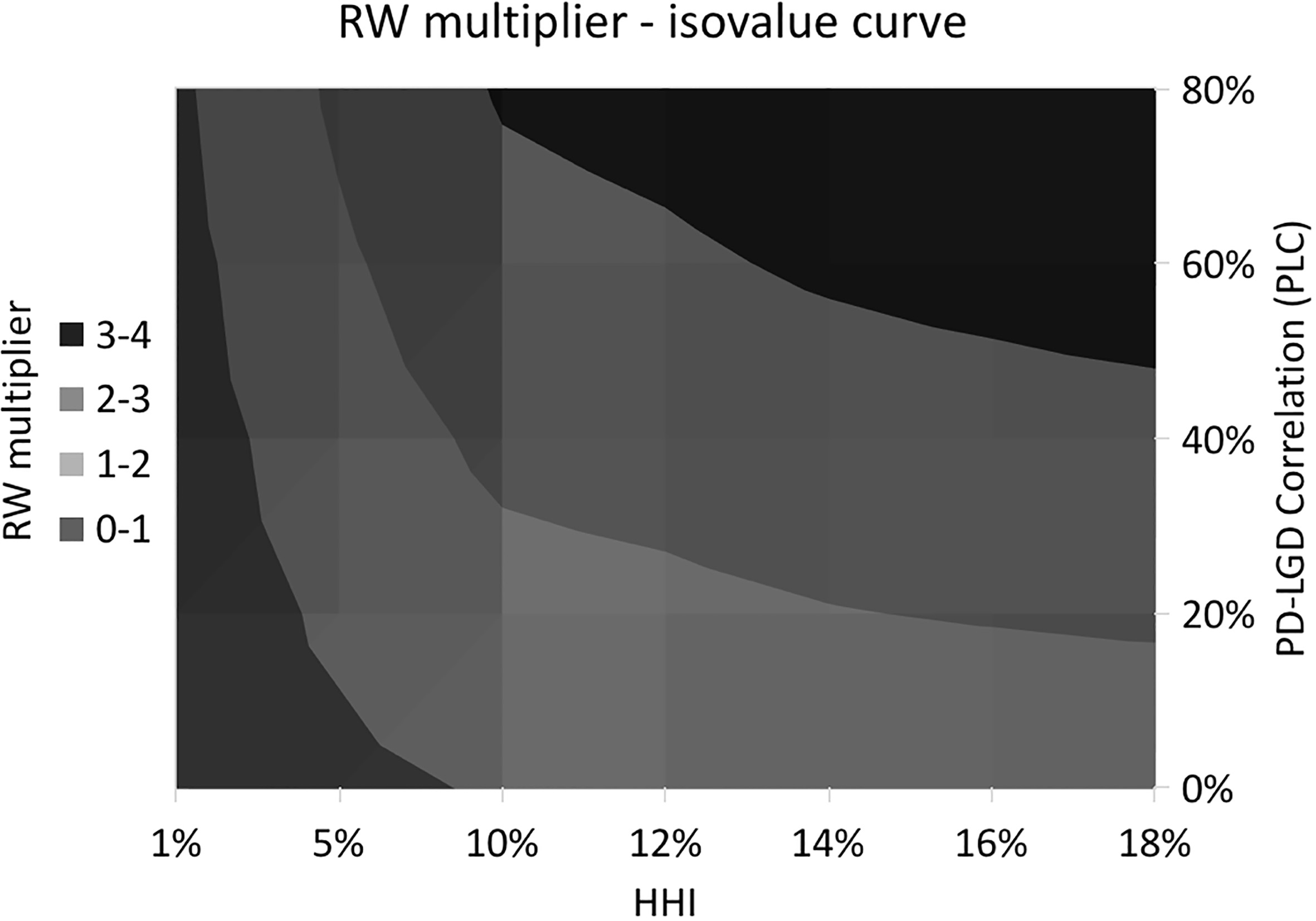

The correlation between LGD and EAD does not require a surcharge to capital. At the same time, it enhances the effect of concentration on capital, though weaker than PD-LGD correlation. The maximum RW multiplier for LEC and concentration is 1.6 as compared to 5.2 as the maximum add-on for PLC and concentration. The low-default portfolio (avg PD $=$ 1%) does not require the capital add-on at all. The results are presented in Table 3.

5.4 Comparison with the add-on proposed by Cyprus and Slovenia regulatory authorities.

Next, compare the markups set by Cyprus and Slovenia regulatory authorities. Their approaches are published in open access so that we can compare their add-on with our results. The Slovenia method does not depend on PLC because the markup is assigned relative to HHI level. One can observe that the Slovenian surcharge for concentration is significantly lower in comparison with our capital markup (Table 4).

Table 4
The Slovenian approach

RW multiplier	HHI
	0%	1%	5%	10%	12%	14%	16%	18%
The Slovenian estimation		1.02	1.06		1.08
Our estimation (without PLC)	1	1	1	1.1		1.2		1.3
Our estimation (with PLC)			1.7	2.4	2.6	2.8	2.9	3

Figure 10.

The CySEC and our estimation of RW multiplier (no PLC).

Figure 11.

The CySEC and our estimation of RW multiplier (with PLC).

The Cyprus add-on is sensitive to PLC for the following reason. The add-on depends on the ratio of loan to capital. We calculate the capital by A-IRB approach (with PLC) and substitute them for Cyprus add-on. One can conclude the following.

First, the CySEC estimates are the most conservative than Slovenian markups and markups proposed in our paper (Fig. 10A and B). Second, our estimates and CySEC surcharges converge to each other with increasing probability of default in a portfolio (compare Fig. 10A and B). A portfolio with a lower probability of default requires higher additional capital because less capital is required for a portfolio with less risk. Consequently, a share of loan exposure in the capital of the low default portfolio is higher than for high default one.

When the PLC is observed in a portfolio, the RWmultiplier is required higher (Fig. 11). The CySEC add-on is not sufficient to cover high concentration for a portfolio with PD higher than 5%. For high-risk portfolio, the markup should be increased up to 3 times compared to CySEC add-on by our estimates.

To sum up the results, we can conclude the following. Capital under the Basel approach, with the constant level of LGD, are sufficient to cover the losses. At the same time, the concentration of the loan portfolio requires a capital surcharge. At the same time, we found that the PD-LGD correlation effect enhances the concentration effect, which can increase the additional capital more than twice for the high level of correlation and concentration. According to our estimation, the markup, offered by Slovenia regulators is insufficient to cover the concentration effect while the Cyprus approach can be able to ensure the capital only for concentration risk but is too low to provide adequate capital for both PLC and concentration effects.

Compare with TLAC amendment that requires holding 16% of RWA since 2019. Then a bank should hold capital at 2 times higher than the current level. We take RW multiplier more than two for 61% of the hypothetical portfolio. It means than in 61% of our cases TLAC add-on is sufficient to cover concentration and correlation risks.

6. Conclusion

We have assumed that the regulators will increase the demand for a capital add-on. First, banking regulators of the United States, for example, Mr Hensarling and Mr Kashkari, concerned about the low capitalization of banks. Second, the Basel approaches are simplified, and therefore unaccounted risks will be covered more by risk weight multipliers rather than sophisticated modelling.

We drew attention to the PD-LGD correlation and concentration as two unaccounted risks by Basel. The researchers have been discussing both risks actively since 2000. Separate capital add-ons were found for each risk. We test the hypothesis that the sum of independent effects is not sufficient to cover the joint effect when both risks happen in a portfolio simultaneously. We check whether Basel capital is adequate to cover the joint effect and propose the risk weight multipliers that can reduce the underestimation.

We generated 640 unique portfolios (64,000 observations running 100 iterations) that correspond to the Basel Committee and S&P findings of an average corporate loan portfolio. Risk weight multiplier estimated as the ratio of modelled risk to Basel capital for each portfolio.

We found that the Basel approach underestimated the effect of PD-LGD correlation and concentration in 1.9 times on average. We show that the joint effect of PD-LGD correlation and concentration requires capital higher in 2.1 times than the sum of two independent effects. The result corresponds to a representative hypothetical portfolio (PD $=$ 5%, LGD $=$ 45%) relative to the most corporate ones according to the paper bcbs256.

We compared estimated RW multipliers with those that set for concentration by Slovenia and Cyprus regulators. The Cyprus method is the most conservative to cover the net exposure concentration effect. However, the Cyprus RW multiplier is not sufficient to ensure capital for the joint effect of concentration and PD-LGD correlation. We also compared our RW multipliers with increased TLAC requirements. We found that increased Basel capital requirements in 2 times are sufficient to cover concentration and correlation risks in 61% of generated portfolios.

As far as we know no work where both risks are combined, and the joint effect of both ones is calculated. Therefore, we can compare our results with the findings of other studies only for independent effects (when a portfolio has only one of two risks). We take that our RW multipliers for PD-LGD correlation differ significantly from (Moody’s, 2012) estimates, equal 1.45, at 5% significance level. At the same time RW multipliers for concentrations higher by 7 and 2 percentage points than the result of BCBS Risk Concentration Group and Gordy and Lütkebohmert (2006), respectively (BCBSWP15, 2006).

We noted that the Basel approach is less sensitive to LGD-EAD than the PD-LGD correlation. The PD-LGD correlation enhances concentration effect stronger than LGD-EAD correlation by 1.75 times (see average RW multipliers from Tables 2 and 3).

We do not provide special estimates for Russian banks. We assume that the average corporate loan portfolio is close to the stylized portfolio specified by the Basel Committee. Therefore, the estimates can be applied to Russian banking regulation.

The study has shortcomings. The RW multiplier estimates can be inflated because we do not consider the historical likelihood of a portfolio with both effects simultaneously. The information is not available. Nevertheless, we expect that the results are most applicable to specialized lending. The BCBS does not deny that PD-LGD correlation characterizes specialized lending. However, it is the Basel recommendation but not the requirements.

The concentration occurs in specialized lending for two reasons. Firstly, there is a concentration of key counterparties. The financial distress can simultaneously move loans from lowest to highest PDs and LGDs. Second, the project finance as the part of specialized lending according to the Basel II/III frameworks is less homogeneous than corporate portfolios. Project finance exposure size varies significantly.

Footnotes

Out-of-scope risks that are not covered in capital requirements: 1. Wrong assumption about asset correlation (R) (see, Khorasgani (2014)); 2. Wrong assumption about normally distributed probability of default; 3. Macroeconomic state is described by a single common latent Gaussian factor, which is a simplification compared to reality (Pykhtin, 2004).

URL: http://www.bis.org/publ/bcbs_wp15.pdf.

URL: http://www.bis.org/publ/bcbs256.pdf.

Both Basel II and III apply the Vasicek model and the same calibration parameters.

URL: www.bis.org/bcbs/publ/d347.htm.

The code used for RW multiplier (add-on) assessment is available upon the request.

URL: http://www.fsb.org/wp-content/uploads/2016-list-of-global-systemically-important-banks-G-SIBs.pdf.

URL: Bank of England, 22–23 February, 2016: http://www.bankofengland.co.uk/research/Documents/ccbs/whfs16/presentation_brierley.pdf.

The code used for RW multiplier (add-on) assessment is available upon the request.

PD $=$ {1%; 5%; 10%; 20%} – 4 values; PLC $=$ {0%; 20%; 40%; 60%; 80%} – 5 values; LEC $=$ {0%; 20%; 40%; 60%} – 6 values; HHI $=$ {0%; 1%; 5%; 10%; 12%; 14%; 16%; 18%} – 8 values.

Acknowledgments

The paper is prepared within the Fundamental Research Program of the National Research University Higher School of Economics (NRU HSE) with the use of the state subsidy ‘5–100’ program for the leading universities of the Russian Federation. The work was conducted in the International Laboratory of Decision Choice and Analysis (DeCAn Lab), Department of Applied Economics of the National Research University Higher School of Economics; Laboratory of Mathematical Modeling of Complex Systems, P.N. Lebedev Physical Institute. We thank the anonymous reviewer for insightful comments.

References

Acharya,

, & Steffen,

(2015, 2). The “greatest” carry trade ever? Understanding eurozone bank risks. Journal of Financial Economics, 115, 215-236.

Altman,

E.I.

Brady,

Resti,

, & Sironi,

(2005). The link between default and recovery rates: Theory, empirical evidence, and implications. The Journal of Business of the University of Chicago, 78(6), 2203.

BCBS. (2006). Basel II. URL: http://www.bis.org/publ/bcbs128.htm.

BCBS. (2011). Basel III. URL: http://www.bis.org/bcbs/basel3.htm.

bcbs_d306. (2015). Capital floors: the design of a framework based on standardised approaches. URL: http://www.bis.org/bcbs/publ/d306.pdf.

bcbs_d362. (2016). Consultative Document Reducing variation in credit risk-weighted assets – constraints on the use of internal model approaches. URL: http://www.bis.org/bcbs/publ/d362.pdf.

BCBS256. (2013). Regulatory Consistency Assessment Programme (RCAP) Analysis of risk-weighted assets for credit risk in the banking book. URL: http://www.bis.org/publ/bcbs256.pdf.

BCBSWP13. (2004). Bank Failures in Mature Economies. Basel Committee on Banking Supervision, 1-69.

BCBSWP15. (2006). Studies on credit risk concentration: An overview of the issues and a synopsis of the results from the Research Task Force project. Basel Committee on Banking Supervision.

10.

Black,

, & Cox,

J.C.

(1976, 2). Valuing corporate securities: Some effects of bond indenture provisions. The Journal of Finance, 31, 351-367.

11.

Carey,

, & Gordy,

(2003). Systematic risk in recoveries on defaulted debt. Federal Reserve Board, Washington.

12.

Chava,

Stefanescu,

, & Turnbull,

(2011). Modeling the loss distribution. Management Science, 57(7), 1267-1287.

13.

Cohen,

, & Costanzino,

(2017, 2). Bond and CDS Pricing with Recovery Risk II: The Stochastic Recovery Black-Cox Model. Risks, 5.

14.

Eckert,

Jakob,

, & Fischer,

(2016, 1). A Credit Portfolio Framework Under Dependent Risk Parameters: Probability of Default, Loss Given Default and Exposure at Default. Journal of Credit Risk, 12.

15.

Ermolova,

M.D.

, & Penikas,

H.I.

(2017). PD-LGD correlation study: Evidence from russian corporate bond market. Model Assisted Statistics and Applications, 12(4), 335-358.

16.

Fischer,

Köstler,

, & Jakob,

(2016, 2). Modeling stochastic recovery rates and dependence between default rates and recovery rates within a generalized credit portfolio framework. Journal of Statistical Theory and Practice, 10, 342-356.

17.

Frye,

Ashley,

Bliss,

Cahill,

Calem,

Foss,

, & Lobbes,

(2000). Collateral damage: A source of systematic credit risk. Risk, 13(4), 91-94.

18.

Giese,

(2005). The impact of PD/LGD correlations on credit risk capital. Risk, 18(4), 79.

19.

Gordy,

(2004). Granularity adjustment in portfolio credit risk measurement. Risk Measures for the 21st Century. John Wiley & Sons.

20.

Gordy,

M.B.

, & Lütkebohmert,

(2013). Granularity adjustment for regulatory capital assessment. International Journal of Central Banking, 9(3), 33-70.

21.

Gordy,

M.B.

, & Marrone,

(2012, 7). Granularity adjustment for mark-to-market credit risk models. Journal of Banking & Finance, 36, 1896-1910.

22.

Han,

(2016). Modeling severity risk under PD-LGD correlation. The European Journal of Finance, 1-17.

23.

Hu,

Y.T.

, & Perraudin,

(2002). The dependence of recovery rates and defaults. Working paper of Birkbeck College.

24.

Jahn,

Memmel,

, & Pfingsten,

(2013). Banks’ concentration versus diversification in the loan portfolio: New evidence from Germany. papers.ssrn.com.

25.

Khorasgani,

, & Gupta,

(2017). Estimating Reserve Requirement for Credit Portfolio of UK SMEs. papers.ssrn.com.

26.

Loutskina,

, & Strahan,

P.E.

(2011, 5). Informed and uninformed investment in housing: The downside of diversification. Review of Financial Studies, 24, 1447-1480.

27.

Meng,

Q.e.

(2010). Implications of PD-LGD correlation in a portfolio setting. Modeling. Methodology. Moody’s KMV.

28.

Miu,

, & Ozdemir,

(2006). Basel requirement of downturn LGD: Modeling and estimating PD & LGD correlations. Journal of Credit Risk, 2(2), 43-68.

29.

Owen,

A.W.

Bryers,

J.S.

, & Buet-Golfouse,

(2015, 3). Hermite Approximations in Credit Portfolio Modeling with Probability of Default-Loss Given Default Correlation. Journal of Credit Risk, 11.

30.

Ozdemir,

, & Miu,

(2008). Basel II implementation: a guide to developing and validating a compliant, internal risk rating system. McGraw Hill Professional.

31.

Penikas,

(2015, 5). History of Banking Regulation as Developed by the Basel Committee on Banking Supervision in 1974–2014 (Brief Overview). Financial Stability Journal, 28, 9-47.

32.

Pykhtin,

(2004, 3). Portfolio credit risk Multi-factor adjustment. Risk London Risk Magazine Limited, 17, 85-90.

33.

Reinhart,

, & Rogoff,

(2009). This Time is Different: Eight Centuries of Financial Folly. Princeton University Press.

34.

Tabak,

B.M.

Fazio,

D.M.

, & Cajueiro,

D.O.

(2011, 11). The effects of loan portfolio concentration on Brazilian banks’ return and risk. Journal of Banking & Finance, 35, 3065-3076.

35.

Vasicek,

O.A.

(1987). Probability of Loss on Loan Portfolio. John Wiley & Sons, Inc., 143-146.

36.

Witzany,

(2009). A two factor model for PD and LGD. SSRN Working Paper. Retrieved from SSRN, 1476305.

The impact of PD-LGD correlation on bank capital adequacy in nongranular loan portfolio 1

Abstract

Keywords

1. Introduction

2. Related literature

2.1 Credit risk modelling in Basel II/III framework

2.1.1 Overview

2.2 The shortcomings of Basel II/III credit risk approach

2.4 PD-LGD correlation

2.6 Paper contribution

3. Simulation study: The joint effect of PD-LGD correlation and exposure concentration

3.1 The joint effect is not a mere of the sum two

4. Methodology

4.1 Generation of 640 of unique hypothetical portfolios

4.3 Portfolio losses

4.4 Capital

4.5.1 Cyprus approach

4.5.2 Slovenian approach

Table 1 Slovenian approach for concentration

5.1 Capital add-on for PLC (PD-LGD correlation)

Table 2 The joint capital add-on for PLC and exposure concentration

Table 4 The Slovenian approach

Footnotes

Acknowledgments

References

Table 1
Slovenian approach for concentration

Table 2
The joint capital add-on for PLC and exposure concentration

Table 4
The Slovenian approach