PD-LGD correlation study: Evidence from the Russian corporate bond market

Abstract

The capital adequacy ratio is one of the important regulatory requirement for banks, which indicates its willingness to cover losses in the event of borrowers’ defaults. The Probability of Default (PD) and Loss Given Default (LGD) are two core parameters of the internal risk rating models used to calculate regulatory capital under the assumption that PD and LGD are independent. Papers based on developed countries data provide evidence the dependence to be positive. It causes that banks underestimate the level of a risk of its loan portfolio, while they do not take into account the existence of such relationship. This is the first paper which aims to estimate the relationship between PD and LGD for Russian public companies. A major conclusion of the research is that using Russian data one cannot argue for the presence of risk parameter dependence whereas research using developed countries’ data suggests there is a positive one. This implies there is no need to overcharge capital for Russian banks compared to their counterparts from developed countries.

Keywords

Basel II the probability of default loss given default PD-LGD correlation credit risk economic capital

1. Introduction

A bank can turn out to be riskier than a regulator recognises. The thing that policymakers are still missing is the positive correlation between probability of default (PD) and loss given default (LGD). The PD-LGD correlation varies from 8 to 80% depending on the sample period and exposure type (please, see Section 2 for more details).

One alternative for a bank to assess credit risk is to estimate probabilities of default for borrowers using bank’s internal models and rely on the Basel Committee’s constant estimate for loss given default.1 When the Basel Committee on Banking Supervision (BCBS) set the same LGD to all loans, the method overlooks the facts that the more likely the borrower is not to pay back on its debt, the more likely the recovered amount is tiny.2 While an economic slowdown boosts default rate, it also increases unsecured loan balances caused by a drop in collateral price. It raises the chance of banks taking higher losses in the event of default. A bank should follow the empirical evidence of PD-LGD correlation to get accurate risk estimates. In other words, a borrower with higher default probabilities should have higher estimates of loss given default. However, the Basel foundation approach for credit risk considers constant LGD acceptable.

According to the Basel standards, only a bank with data observation period more than seven years can replace constant LGD by risk-sensitive one (derived from internal statistical models).3 There are greater deeps beyond. The data should be consistent with Basel default definition. For instance, only a few Russian banks applied a strict default definition in compliance with Basel standards before starting Basel implementation in Russia (2012).4 The Russian example represents that a bank in developing country where risk regulation was initially far from the Basel standards can require more time to implement risk-sensitive LGD. Since 2009 14 countries joined the Committee; 10 out of 14 new members were developing countries.5 Then the problem to introduce risk-sensitive LGD can arise for about 10 out of 27 BCBS members.

Applying risk-insensitive LGD (i.e. neglect PD-LGD correlation) a bank may underestimate credit risk. Thus, a bank holds inadequate capital to cover losses if borrowers do not pay back loans. Miu and Ozdemir, (2006) conclude the Basel constant LGD benchmark should be raised by 35–45% to provide adequate capital. Moodys (2010) suggests recouping PD-LGD correlation by raising capital by 45%. In 2011 the Basel III tightened the capital requirements (Common Equity Tier I 4.5% against 2%, Tier I 6% against 4%) and added buffers (the capital conservation buffer, the countercyclical buffer, and G-SIFI surcharge). The capital conservation buffer (from 0% to 2.5%) should cover the losses in recessions when assets write-down is significant. The last one is close in meaning to capital add-on for PD-LGD correlation expected by experts. In result, a bank is required to hold 8% of risk-weighted assets (hereafter RWA) as the total capital and 2.5% of RWA as the capital conservation buffer (not taking into account the remaining buffers designed to cover other risks). One can argue the Basel III made the capital requirements stricter, but it is still not able to compensate the capital shortfall that Moodys (2010) found studying the PD-LGD correlation. The minimum capital requirement should be higher by 1.1 percentage points to cover PD-LGD correlation risk fully according to Moodys (2010) estimates.6

One cannot but agree that the US and the European Union ensure adequate capital for PD-LGD correlation problem through the introduction TLAC and MREL. TLAC doubled the capital requirements for 30 G-SIBs (16% against the Basel 8%, 18% since 2022). The Russian banks have not yet obtained the permit to use IRB approach (as of 01/07/2017). Therefore, the banks and regulator have not yet faced the PD-LGD correlation problem. Therefore, the Russian regulator should also understand what is the lower bound of capital requirements that will be sufficient to cover bank risks including the PD-LGD correlation problem. For instance, the US study (Moodys, 2010) shows that the capital requirements cannot be less than 11.6% to take into account the PD-LGD correlation problem. Therefore, there exists a demand to study the correlation on the Russian market too.

We hypothesize that the PD-LGD correlation and the amount of extra capital can differ among the Basel jurisdictions. The proposal followed after the BCBS publication ‘d297’ that disclosed the national discretions in banking regulation in respect of Basel standards caused by the local peculiarities.7 We found the need to study whether the national discretion is relevant to apply for extra capital resulting from PD-LGD correlation. Having differences in the correlation in the US and Russia, we can judge that the uniform regulation concerning extra charges on the capital is not applicable. The majority of previous works implemented PD-LGD correlation into capital adequacy models and assessed its impact on the capital. They applied the PD-LGD correlation value (51%, Altman et al., 2005) found in the US corporate bond market. Our work expands the knowledge of the PD-LGD correlation geographically. We studied the Russian case. We have not found the PD-LGD correlation on Russian corporate bond market. This implies there is no need to overcharge capital for Russian banks compared to their counterparts from developed countries. It means that the national discretion takes place. The work also has practical value for the Russian regulator to understand sufficiency of the PD-LGD correlation in Russia and its influence on the capital.

We analyze unbalanced panel data of 839 Russian corporate bond issuers during 2000–2015 (16 years). The PD-LGD correlation should be studied over the long-run period for the following reason. A bank estimates the average long run capital requirements to avoid capital fluctuations over economic cycle because capital raising is expensive. Therefore, the capital add-on for the PD-LGD correlation should be assessed based on the long run relationship between PD and LGD. The period of 2000–2015 is sufficient because it includes two economic cycles in Russia (2000–2009, 2010–2015).

We use corporate bonds instead of bank loans because there is no available public data about workout LGD of bank loans. At the same time, LGD for bonds can be assessed using a market approach that determines the bond price after default as a proxy of recovery (Bhatia, 2006, p. 285, cited by Seidler, 2008). The approach complies with the previous works. Our methodology does not mean that the most Russian banks hold bonds. A reader can imagine that there is a bank that consists of borrowers similar to those who take public loans. A public loan often belongs to a large company; then we study the correlation that complies mostly with the corporate portfolio of a major bank.

The paper contributes to the literature in the following ways. First, the paper has practical value for the Russian regulator and banks to understand sufficiency of the PD-LGD correlation in Russia and its influence on the capital of the Russian banks. Second, the paper expands the knowledge of the PD-LGD correlation geographically. There is a high variance of the PD-LGD correlation estimates (from 0% to 80% depending on exposure types, observation period, and region). It can lead to high variance of risk-weighted assets (and capital, consequently) across jurisdictions. The last problem is the Basel Committee’s great concern which was described in the document ‘bcbs256’. The Committee is finding the reason for high variance. If the PD-LGD correlation can be one of the possible reason, there exists a demand to explain the stronger correlation in one case and weaker one in others. As we know, we add Russia as the third case after the US and Czech Republic into the list of regions where PD-LGD correlation has been assessed. We found that there is statistically insignificant PD-LGD correlation on the Russian corporate bond market. If the high variance of the correlation will be confirmed for most countries, then high RWA differences across jurisdictions are rather natural (local economy peculiarities) than artificial (model assumptions, methods, and etc.). Third, our study can be further confirmation that the uniform capital regulation is not applicable for countries with significant differences in the development level. The proposal followed after the BCBS publication ‘d297’ that disclosed the national discretions in banking regulation in respect of Basel standards caused by the local peculiarities. Having differences in the correlation in the US and Russia, we can judge that the uniform regulation concerning extra charges on the capital is not applicable. We have not found the PD-LGD correlation on Russian corporate bond market. This implies there is no need to overcharge capital for Russian banks compared to their counterparts from developed countries. It means that the national discretion takes place.

This paper is organized in the following way. Section 2 provides an overview of research on the relationship of PD and LGD and an overview of approaches for assessment of the probability of default. Section 3 includes a description of the data used and also an initial list of risk factors used to build a model of PD. Sections 4 and 5 are devoted to modelling the probability of default and loss given default, respectively. Section 6 presents results on the relation between default probability and the loss given default for the Russian corporate bond market. Section 7 is the conclusion.

2. Literature review

The literature review consists of two parts. The first part describes the results of previous works which estimate the PD-LGD correlation over different sample period and for various exposure types. The second part presents the impact of the correlation on capital.

A bank calculates a capital using the Vasicek model (Vasicek, 2002). However, the model does not consider the correlation between PD and LGD. It means that the capital is underestimated. The Basel II standards do not describe explicitly the requirements to take into account PLC (PD-LGD Correlation) in capital requirements. The Basel Committee admits PLC only for specialized lending exposures (BSBC, 2001), but the share of specialized lending is small enough compared with the corporate sector so that the assumption about dependence PD and LGD is not applied for a large part of the credit portfolio.

The problem of the PD-LGD correlation has been studying since 2001. The positive connection of PD and LGD is the most common result (the exception is the paper (Carey and Gordy, 2003)). All studies about PD-LGD relationship examined in literature review here (besides (Witzany, 2011)) are based on US data over 1980–2010.8 The probability of default was considered ex-post as the realized annual default rate. The default rate is determined as the number of defaulted bonds over the total number of outstanding bonds on the US market, or as a percentage of issue volume of bonds that were defaulted to the total volume. LGD is estimated using both a market approach, based on bond prices after default, and the average discounted ultimate recovery rate provided by rating agency Moody’s since 1987. Database Moody’s is the only international source of recovery rates with complete data. However, there is no data about Russian bond market. That is the reason why so far there were no studies about PD-LGD correlation for Russia.

The correlation is observed on average instrument-level LGD and default rate by year. LGD can be modelled by workout or market methods. There is another approach to examine the correlation on firm-level recoveries, suggested in Carey and Gordy, (2003) where the main idea is that systematic risk is focused on variations in the value of bankrupt firms.

As it was mentioned above the initial step to study PD-LGD correlation problem was to decline permanency of LGD over a business cycle. In the paper (Gupton and Stein, 2002) a multifactorial LGD model LossCalc was constructed on 1,800 observations (900 public and non-public companies) using recovery rate of defaulted loans, bonds and preferred shares, covering the period from 1981 to 2000. In the study parameter LGD consider for different types of collateral for loans (secured, senior unsecured, subordinate). The market value of the defaulted instrument at the expiration of 1 month after the default was a proxy for recovery. The longer time after default period, the more difficult to determine the cash flow of the overdue debt or the value of a financial instrument. The authors found a strong correlation between changes in GDP and changes in recovery rates. The authors emphasize that recovery occurs at different times in different industries.

In the work (Altman et al., 2004) the negative correlation between default rate and recovery rate was found for U.S. defaulted bonds for the period from 1982 to 2000. The authors improved the model by including the supply of defaulted bonds in the model of recovery rate assessing. Recovery rate was found on the aggregated data by bond seniority and collateral value. The work also shows a significant impact of return level in the financial market in forecasting recovery rate, but small relationship between RR and GDP (the result does not coincide with the study (Gupton and Stein, 2002)). The study was also presented a literature review about the problem of PD and RR relationship, which includes the early works of Frye, (2000); Jarrow, (2001); Jokivuolle and Peura, (2000); Hu and Perraudin, (2002); Bakshi et al., (2001).

In the study (Dullmann and Trapp, 2004) the authors have shown that the loss given default determined by market approach is more sensitive to changes in systematic risk factor than workout LGD. Thus, a choice of the method of calculating the LGD determines the value of economic capital. Workout LGD leads to underestimated economic capital for a bank. The study was conducted on the data presented in the form of time series of default rate and the recovery rate received from Standard and Poor’s Credit Pro database. The sample includes bonds and loans for the period from 1982 to 1999. The model suggests that recovery corresponds to the log-normal distribution.

Giese (Giese, 2005) builds a nonlinear model based PD and LGD data on U.S. bonds over the period from 1982 to 2001. The result of the positive correlation of the two parameters is consistent with the results of other studies.

The study (Witzany, 2011) differs from other works discussed above because the dependence of PD and LGD is checked for data of retail loans portfolio of one of the largest Czech banks. Data were obtained for the period from 2002 to 2008. The results confirm a weak positive correlation between PD and LGD (0.0775). The author suggests that the weak statistical significance is due to the short sample including only seven years.

In the work (Altman, 2006) working paper (Carey and Gordy, 2003) was mentioned where preliminary results of the study, in contrast, specify the lack of correlation between PD and LGD data for 1970–1999. However, assessing the relationship of the components in separate periods of time (for example, 1988–1998) the dependence was found. The study notes that the weak or asymmetric relationship between PD and RR can be explained by the fact that these two components are influenced by various macroeconomic factors.

In research (Chava et al., 2011) it was found that the magnitude of the correlation varies depending on the credit cycle.

The following works show the impact of correlation on a value of the capital of a bank.

The empirical work (Meng et al., 2010) by Moody’s is devoted to the study of the influence of correlations between PD and LGD on risk indicators and profitability of a loan portfolio. The authors show that MTM (market-to-market value) will be lower with a non-zero correlation between PD and LGD. The asset price decreases to reduce systemic risk return. As a consequence, spread of a credit instrument increases. Their numerical experiment shows that stressed LGD recommended by the Basel II is not a conservative value to calculate capital adequacy.

The authors (Miu and Ozdemir, 2006) observed a higher sensitivity of economic capital to changes in specific risk compared with the changes of a systemic risk. Moreover, the influence of specific factors is expressed stronger at high correlation between PDs of different borrowers. Economic capital is highly sensitive to the correlation between PDs of different borrowers, but it is not significant in the case of zero correlation between LGD and PD of the borrowers even if the correlation between PD and LGD is strong. Miu and Ozdemir, (2006) conclude the Basel constant LGD benchmark should be higher by 35–45% to provide adequate capital.

Our study extends the existing literature in two main directions. First, our study is the first one that examines the relationship between probability of default and loss given of default for the Russian corporate bond market. We show the difference in PD-LGD correlation for developed and emerging countries using Russian example. Second, an accurate estimation of capital is a topical issue for Russian regulator. We present the evidence that zero PD-LGD correlation on Russian market does not require additional capital.

Fig. 1.

The distribution of defaults of corporate bonds (default and non-execution of put option (puttable bond)) over the period 1999–2015.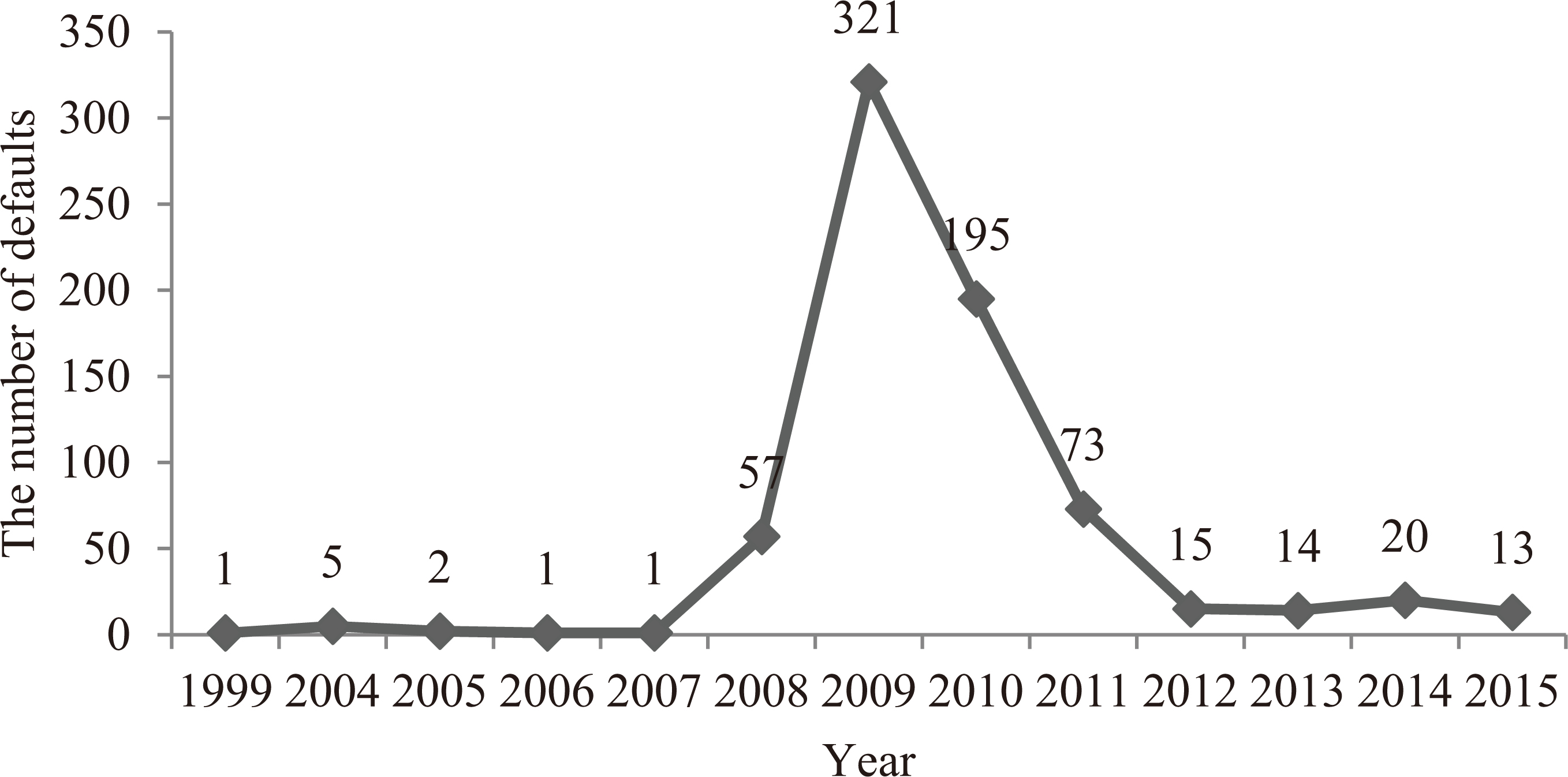

3. Data

3.1 Data for PD estimates

We analyze unbalanced panel data of 839 Russian corporate bond issuers during 2000–2015 (16 years). The sample consists of 6 688 issuer-years observations. Data come from three sources. We obtain information about corporate bond defaults from ru.cbonds.info, information about issuers’ balance sheets and income statements from spark-interfax.ru, information about bond prices and its face values from Moscow Exchange database. The starting point of our sample is defined by data availability in ru.cbonds.info.

Eight hundred and thirty-nine issuers represent 60% of all Russian corporate bond issuers during 2000–2015. The remaining 40% of issuers were excluded from the sample because they did not have financial statements (Russian GAAP) in any of the years over 2000–2015. The sample consists of 54% of unique issuers who have at least one default in general population. The other defaulted companies have no available financial data published 12- and 24- months before default. The default rates of general population and sample differ insignificantly.

The graph 1 only the period from 2008 to 2014 is the most representative (the realized default rate is more than 0%). For instance, the US time series of the annual default rate are available over 20 years. The time series for Russia consists of only 7 points that makes impossible to estimate the correlation using annual market data. Therefore, the PD-LGD correlation is estimated using PDs and LGDs of borrowers in the sample.

Financial indicators (annual balance sheet, annual profit and loss statement) were extracted from SPARK. SPARK was chosen as the most representative database for Russian companies compared with Moody’s, FIRA-PRO, and Ruslana.

We apply the following data preprocessing. If the company has zero total assets, the company was excluded from the analysis, because in the most cases, the absence of data about total assets means omissions of other financial indicators. Table 1 represents the result of data preprocessing. The final sample included 201 defaulted observations. The number of defaults is larger than the number of defaulted companies because a company can multiple defaults in different years.

Table 1
The distribution of defaulted and non-defaulted companies in both initial and final samples.9
⁹
As comparison with the previous version of research the sample was expanded by 2642 observations having panel data structure.

	Before data processing				After data processing
Year	Non default	Default	Total	Sample default rate	Non default	Default	Total	Sample default rate
2000	839	0	839	0%	220	0	220	0%
2001	839	0	839	0%	241	0	241	0%
2002	839	0	839	0%	255	0	255	0%
2003	839	0	839	0%	281	0	281	0%
2004	836	3	839	0%	325	0	325	0%
2005	838	1	839	0%	367	0	367	0%
2006	838	1	839	0%	425	1	426	0%
2007	838	1	839	0%	509	0	509	0%
2008	804	35	839	4%	531	30	561	5%
2009	739	100	839	12%	477	83	560	15%
2010	775	64	839	8%	525	44	569	8%
2011	815	24	839	3%	542	20	562	4%
2012	833	6	839	1%	547	6	553	1%
2013	831	8	839	1%	547	8	555	1%
2014	830	9	839	1%	513	9	522	2%
2015	839	0	839	0%	182	0	182	0%
Total	13,172	252	13,424	2%	6,487	201	6,688	3%

Note: the first part of the table “Historical data” provides the information about the data received from the SPARK database prior to the removal of missing values; the second part presents the information about the final sample after removal of missing values.

Table 2

The percentage of missing bond prices

Days before/after default	The numbers of observations of bond price	The percent of missing values
90 days before default	114 out of 140 defaults	19%
60 days before default	109 out of 140 defaults	22%
30 days before default	108 out of 140 defaults	23%
At moment of default	93 out of 140 defaults	34%
30 days after default	74 out of 140 defaults	47%
60 days after default	67 out of 140 defaults	52%
90 days after default	78 out of 140 defaults	44%

The data for macroeconomic variable (consumer price index and GDP) was extracted from Federal State Statistics Service. The variables are included in PD models.

3.2 Data for LGD

LGD is determined using the bond price after default as a proxy of the recovery. There are two sources from which information about prices and their nominal value of bonds was taken. The first one is research of Antonova (Antonova, 2013), which contains recovery rates in 30 and 90 days after default for 59 emitters over the period 2006–2010. The second source is Moscow Exchange Information Service. Firstly, it is used to gather missing information about the bonds’ prices in 60 days after the defaults from the Antonova’s list, and also to find the same prices at 30, 60, 90 days before default. We estimate the PD-LGD correlation for different time horizon to observe the moment when the correlation enhances. The event of default is a planning date of execution of the obligation by a borrower.

We add the new defaults occurred from 2012 to the second quarter of 2015 (there are no defaults in 2011) and some defaults over the period from 2002 to 2010 that was not specified in the research (Antonova, 2013). Eurobonds are excluded from samples because there is no available information about bond prices in Moscow Exchange Information Service. Therefore, the work sample includes 140 defaults.

The missing values were mostly for bonds after default. The trading of defaulted securities declines on the exchange and the bond price can remain unchanged after default. Then the recovery can be overestimated being assessed through a bond price. It means that the market information could not reflect the true recovery. The final sample also includes 17 cases when bond prices were not observed at all (due to the lack of trading). Table 14 shows that the prices are mostly decreasing. There are also cases when the prices remain unchanged and even increase.

Table 3
The descriptive statistics of recovery rates based on bond prices

	Numb. of obs.	Min	Max	Mean	Median	Stand. deviation
RR ( $-$ 90 days)	114	12.40	100.34	80.09	90.00	23.60
RR ( $-$ 60 days)	109	2.28	110.00	73.71	80.00	25.57
RR ( $-$ 30 days)	108	0.35	102.00	66.77	71.00	27.90
At time of default	93	4.63	100.00	59.29	57.49	27.80
RR ( $+$ 30 days)	74	1.59	101.00	46.43	50.00	26.92
RR ( $+$ 60 days)	67	0.41	99.00	38.06	34.85	27.50
RR ( $+$ 90 days)	78	0.01	100.00	44.08	44.41	33.30

Note: $-$ 90 days means 90 days before default, $+$ 90 days means 90 days after default.

Ending the bond trade on the exchange made complicated to fix the bond quote after a certain number of days after/ before default. Table 4 shows that the average number of days and the median coincide with the planned number of days before and after the date of default. However, there are observations for which bond price is available through 211 days of 90 days after the default (RU000A0JP8M9). It means that there is a small bias in recovery that we used in our research.

Table 4

The numbers of actual days before/after default

	Numb. of obs.	Min, days	Max, days	Mean, days	Median, days	Stand. deviation, days
For $-$ 90 days	114	44	173	91	90	12
For $-$ 60 days	109	36	72	58	60	6
For $-$ 30 days	108	8	55	30	30	6
For $+$ 30 days	93	14	77	31	30	7
For $+$ 60 days	74	33	99	61	60	7
For $+$ 90 days	67	51	211	94	90	17

Note: $-$ 90 days means 90 days before default, $+$ 90 days means 90 days after default.

4. Probability of default

In compliance with the definition of Basel II, the default is defined as a case when the debtor is past due more than 90 days on any material credit obligation to the banking group. The delay in 90 days was monitored through the scheduled and actual date of bond execution using Cbonds.info. Financial indicators of companies corresponding to the prior year’s figures before the default. It is broadly in line with the regulatory requirement.

We examine the period from 2000 to 2015. The western sanctions on Russia was introduced in March 2014. We suppose that the fact that we did not address western sanctions has no significant impact on the paper’s result for the following reasons.

•
Part of the sanctions were realized against individuals and state companies. Our sample does not include the municipal or state bonds. We focus on corporate bonds.
•
We expect that a financial statement reflects the individual effect of western sanctions on a non-state company. Then the PD model reacts on western sanctions through the financial indicators.
•
We expect that the common effect of western sanctions on the industries is taken into account by the variable ‘GDP growth’.
•
The sample for the PD-LGD correlation is smaller than the sample for PD model development, because it includes only default observations with known LGD outcomes. In 2014–2015 the defaults of some companies (e.g. Transaero) subject to sanctions occurred, because they did already the financial problem.
•
Sections 4.1–4.3 present that the ROC curve is ranged from 62% to 90% that indicates high discriminatory power of PD models. Then the fact that we did not address western sanctions has no significant impact on the paper’s result for the following reasons.

The sample was divided into two parts to develop and validate PD model, respectively. The model risk drivers were selected after review the articles (Altman, 1968, 1977); (Ohlson, 1980); (Bandyopadhyay, 2006); and (Totmjanina, 2011). The full list of financial indicators with economic interpretation and the expected impact on PD is presented in Table 12, Appendix. The short list consists the factors with fewer missing values and high discriminatory power (Table 13, Appendix).

The multicollinearity was reduced by orthogonalization. It was also decided to remove liquidity and return indicators due to extremely high VIF (variance inflation factor). VIF values showed that liquidity ratios were highly correlated among themselves and with retained earnings weighted by the size of total assets. Despite the fact that in most cases profitability reflects the efficiency of companies’ activities, in the case of default explanation these parameters play a minor role, i.e. the dependence between default and profitability is low, which is consistent with the findings of Totmjanina (2011) (1).

Fig. 2.
The distribution of default rate in training and testing samples.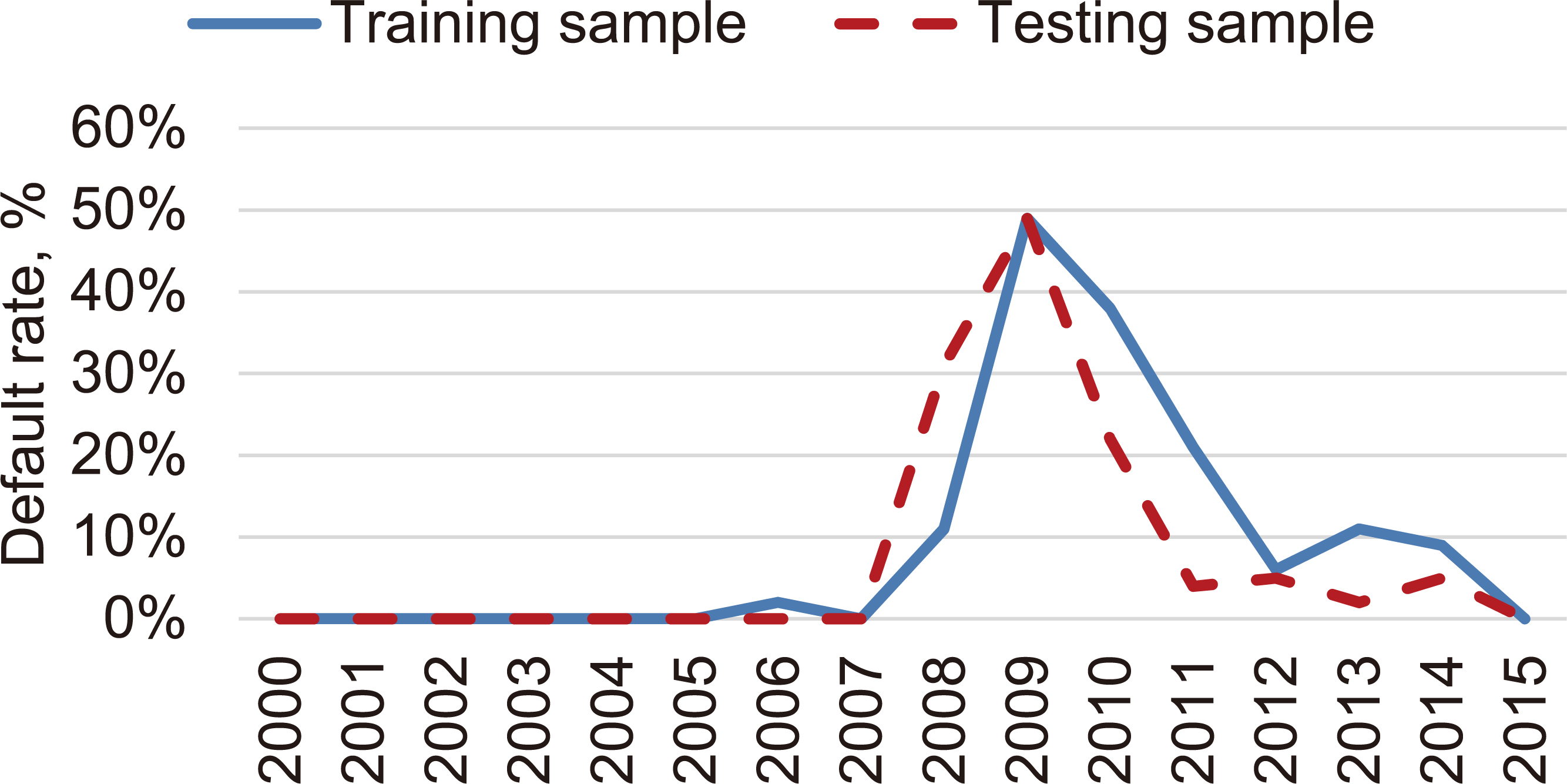

Fig. 3.
The number of observation with default and no default in training and testing samples.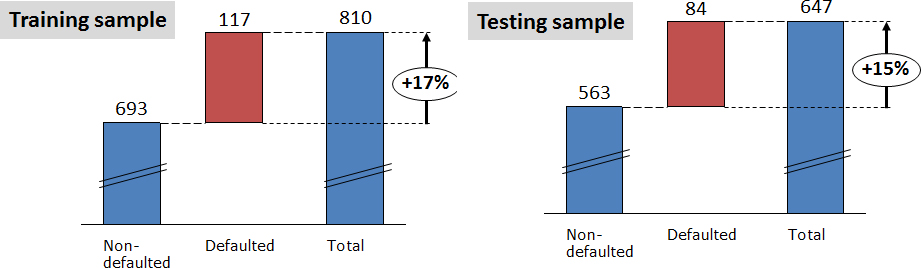

4.1 PD model: Out-of-sample

Out-of-sample implies that the data for the testing sample (not involved in a training process) is selected from the original sample randomly. There is no restriction on the time of default and the type of subsampling. The only condition is that the training and testing samples do not overlap.

One observation for each borrower is randomly selected for each of two subsamples. The selection algorithm is constructed so that if the borrower was in default, then defaulted observation is placed to final sample. This is done to ensure the sufficient number of defaults for the training and testing samples to build the model with an acceptable level of discriminatory ability and accuracy of the estimates. The majority of defaults, which will be further used to evaluate the relationship between PD and LGD, were assigned to the testing sample. These defaults are characterized by the fact that they have more information about recovery rate than those defaults that are left in the training set.

Table 5 provides PD model specifications. The model extends gradually by macroeconomic variables, the logarithms of variables, the squares of the variables. The following parameters are monitored: statistical significance of the coefficients, the coincidence of the coefficient’s sign with the sign of the observed correlation of the dependent and independent variable, the accuracy of the model (pseudo R2) and the discriminatory ability of the model estimated using the AUC.

Table 5
The stages of PD model development (out-of-sample)

	(1)	(2)	(3)	(4)	(5)
VARIABLES	Basic	Basic $+$ macro	Basic $+$	Basic $+$	Basic $+$
			macro $+$ ln	macro $+$ sq	macro $+$ sq $+$ ln
Capital to account payable	$-$ 0.579***	$-$ 0.574***	$-$ 0.885*	$-$ 0.761***	$-$ 1.227***
	(0.184)	(0.186)	(0.483)	(0.188)	(0.468)
Current liabilities to current assets					0.0688***
					(0.0247)
Fixed assets to liabilities (squared)				$-$ 2.169**
				(0.966)
Current assets (logarithm)					0.173*
					(0.0937)
Sales to total assets	$-$ 0.555***	$-$ 0.506***	$-$ 0.816***	$-$ 0.525***	$-$ 0.989***
	(0.184)	(0.183)	(0.286)	(0.190)	(0.316)
Consumer price indes		0.163***	0.199***	0.169***	0.196***
		(0.0396)	(0.0442)	(0.0393)	(0.0459)
Accounts payable (logarithm)			0.257***		0.121**
			(0.0455)		(0.0597)
Indicator of positive or negative net	1.326***	1.309***	1.545***	1.369***	1.428***
profit (binary variable)	(0.231)	(0.238)	(0.272)	(0.236)	(0.281)
Cash flow to total assets (logarithm)			$-$ 0.209***		$-$ 0.250***
			(0.0503)		(0.0546)
GDP growth		$-$ 5.749***	$-$ 6.110***	$-$ 5.994***	$-$ 5.616***
		(1.183)	(1.341)	(1.178)	(1.388)
Current assets to liabilities	$-$ 0.589***	$-$ 0.425*	$-$ 0.506*		$-$ 0.879***
	(0.216)	(0.224)	(0.302)		(0.299)
Working capital to total assets	0.371***	0.341***	0.756***	0.430***	0.852***
	(0.130)	(0.125)	(0.262)	(0.130)	(0.281)
Accounts receivables to debt (logarithm)					0.417***
					(0.0960)
Fixed assets to liabilities		$-$ 1.221**	$-$ 1.566**
		(0.606)	(0.683)
Cash flow to total assets	$-$ 7.828*	$-$ 8.665**		$-$ 9.184**
	(4.191)	(4.207)		(4.268)
Constant	$-$ 1.548***	$-$ 18.53***	$-$ 28.53***	$-$ 19.22***	$-$ 28.81***
	(0.188)	(4.230)	(5.006)	(4.203)	(5.385)
Observations	774	774	744	766	743
Pseudo R-Squared	0.229	0.273	0.364	0.262	0.408
Area under ROC curve (training data)	0.829	0.852	0.898	0.844	0.912
Area under ROC curve (testing data)	0.757	0.781	0.802	0.765	0.787
Sensitivity	20	24.35	39.25	24.35	49.53
Specificity	97.27	97.42	96.86	97.70	97.64
Correctly classified	85.79	86.56	88.58	86.68	90.71

Standard errors in parentheses. *** $p<$ 0.01, ** $p<$ 0.05, * $p<$ 0.1.

Table 6 shows that VIFs are acceptable.

Table 6

VIF of explanatory variables

Variable	VIF
Equity to accounts payable	1.52
Current assets to current liabilities	1.42
Current assets (logarithm)	2.21
Sales to total assets	1.02
Consumer price index	2.51
Accounts payable (logarithm)	2.49
Indicator of positive or negative net profit (binary variable)	1.08
Cash flow to total assets (logarithm)	1.14
GDP growth	2.5
Current assets to loabilities	1.06
Working capital to total assets	1.45
Accounts receivables to debt (logarithm)	1.26

Table 7

The stages of PD model development (out-of-time)

VARIABLES	(1)	(2)	(3)
	Basic	Basic $+$ macro	Basic $+$ macro $+$ ln
Current assets to liabilities			$-$ 1.029***
			(0.342)
Cash flow to total assets	$-$ 10.06***	$-$ 6.116**	$-$ 6.355*
	(3.498)	(2.960)	(3.817)
Fixed assets to liabilities	$-$ 1.256**	$-$ 1.498***	$-$ 1.431*
	(0.542)	(0.542)	(0.748)
Sales to total assets	$-$ 0.560**	$-$ 0.571**	$-$ 1.221***
	(0.222)	(0.222)	(0.332)
Indicator of positive or negative net profit (binary variable)	1.080***	1.114***	1.245***
	(0.237)	(0.236)	(0.289)
Consumer price index			0.140**
			(0.0636)
Accounts receivables to debt (logarithm)			0.472***
			(0.100)
Current liabilities to current assets			0.0192*
			(0.0110)
Current assets (logarithm)			0.254***
			(0.0811)
GDP growth		$-$ 3.022***	$-$ 4.327***
		(0.747)	(1.341)
Capital to account payable	$-$ 0.677***
	(0.244)
Constant	$-$ 1.328***	$-$ 1.056***	$-$ 20.05***
	(0.197)	(0.211)	(7.172)
Observations	722	722	562
Pseudo R-Squared	0.199	0.212	0.354
Area under ROC curve (training data)	0.804	0.819	0.885
Area under ROC curve (testing data)	0.716	0.621	0.734
Sensitivity	3.810	22.86	48.51
Specificity	99.84	96.60	95.88
Correctly classified	85.87	85.87	87.37

Standard errors in parentheses. *** $p<$ 0.01, ** $p<$ 0.05, * $p<$ 0.1.

Despite the fact that from an economic point of view an industry seems important variable, the analysis showed that this variable is not statistically significant. The model No 5 (Table 5) is characterized by the highest R2 pseudo value. The interpretation of the variables of the model 5 is included in Section Appendix.

4.2 PD model: Out-of-time

Out-of-time sample division means that training dataset prior to a certain date in the past is selected, while the testing sample is formed by the data after the selected date. There is sample division into two parts (training and testing subsamples) by the time criterion:

1.
Training sample: 2000–2010
2.
Testing sample: 2011–2015

For out-of-time model squared variables were not statistically significant. The variable “industry” is not statistically significant as in out-of-sample model.

Table 8 shows that VIFs are acceptable.

Table 8
VIF of explanatory variables

Variable VIF

Current assets to liabilities 1.36

Cash flow to total assets 1.03

Fixed assets to liabilities 1.08

Sales to total assets 2.25

Indicator of positive or negative net profit (binary variable) 1.49

Consumer price index 1.58

Accounts receivables to debt (logarithm) 1.87

Current liabilities to current assets 2.35

Current assets (logarithm) 3.06

GDP growth 1.62

Capital to account payable 1.54

Accounts receivables to debt (logarithm) 1.54

Fig. 4.
The number of observation with default and no default in training and testing samples.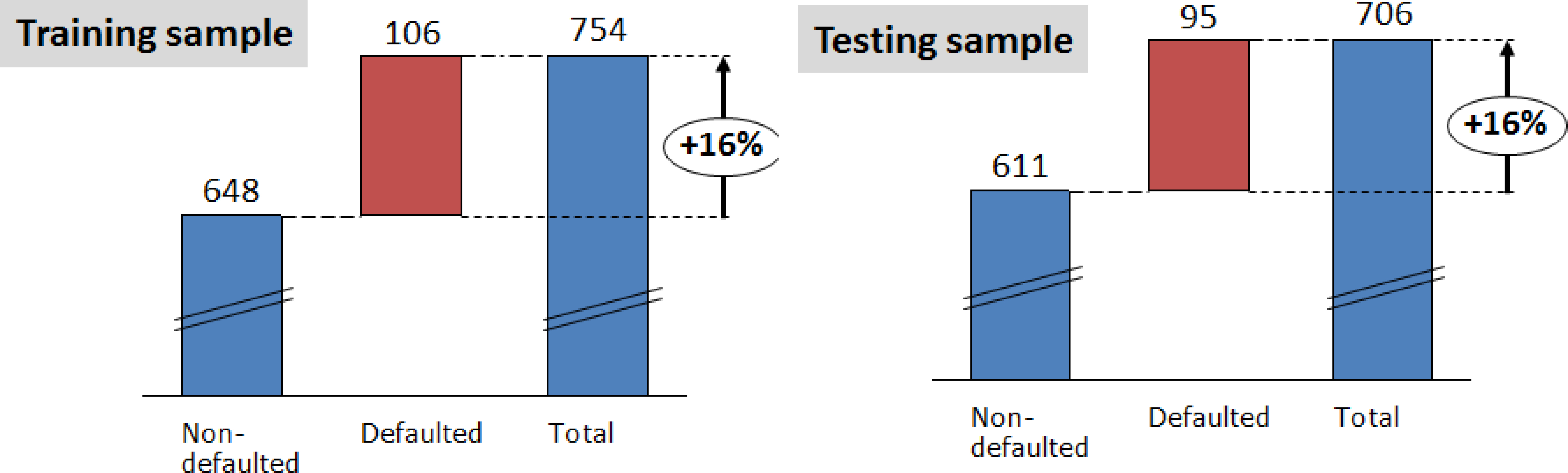

4.3 PD model: Panel data

Variable	VIF
Current assets to liabilities	1.36
Cash flow to total assets	1.03
Fixed assets to liabilities	1.08
Sales to total assets	2.25
Indicator of positive or negative net profit (binary variable)	1.49
Consumer price index	1.58
Accounts receivables to debt (logarithm)	1.87
Current liabilities to current assets	2.35
Current assets (logarithm)	3.06
GDP growth	1.62
Capital to account payable	1.54
Accounts receivables to debt (logarithm)	1.54

Model of the probability of default can be built based data with a panel structure that combines cross-sectional data and time series. Panel data allows taking into account unobserved individual characteristics of companies and considering their heterogeneity.

The logit regression with fixed effects assumes that the analysis will be performed based on only the company with the dependent variable (i.e. the incident of default) that at least 1 time changed during 1999 to 2014 (exhibit variation in the values over time). Therefore fixed effects model will drop 4566 observations from 6487 observations (70% of the sample). Following the study (Cameron and Trivedi, 2005; op. CIT. by Fantazzini, 2008), the logit models with fixed effects have a significantly lower efficiency of forecasting due to “uselessness” of data with a constant of zero in the dependent variable (the company without default). Therefore, in this paper pooled regression and regression with random effects will be examined. The initial sample was divided into training and testing samples (80% and 20%, consequently) by the out-of-sample approach.

Table 9
Regression output: pool regression and regression with random effect

VARIABLES	Corr (lag_default, X)	Pool logit model	Logit model with random effect
Sales to total assets	$-$ 0.0051	$-$ 0.4916***	$-$ 0.5150**
		(0.1832)	(0.2195)
Indicator of positive or negative	0.1182	1.3060***	1.2614***
net profit (binary variable)		(0.2006)	(0.2516)
Working capital to total assets	0.0049	0.3050**	0.3810**
		(0.1304)	(0.1586)
Cash flow to total assets	$-$ 0.0481	$-$ 11.7277***	$-$ 11.2818**
		(4.4264)	(4.6585)
Fixed assets to liabilities	$-$ 0.0029	$-$ 2.2917***	$-$ 3.1781***
		(0.5763)	(0.8182)
EBIT to total assets	$-$ 0.0001	$-$ 0.3102**	$-$ 0.3669**
		(0.1274)	(0.1589)
Consumer price index	0.1480	0.1112***	0.1643***
		(0.0297)	(0.0369)
GDP growth	$-$ 0.0592	$-$ 4.0334***	$-$ 5.4804***
		(0.8862)	(1.1101)
Constanta		$-$ 15.1129***	$-$ 22.0612***
		(3.1804)	(4.0305)
/lnsig2u			1.3449
			(0.2662)
sigma_u			1.9591
			(0.2608)
rho			0.5384
			(0.0662)
AUC (training sample)		85% (standard error 0.0158)	85% (standard error 0.0157)
AUC (testing sample)		77% (standard error 0.0224)	78% (standard error 0.0219)

Standard errors in parentheses. *** $p<$ 0.01, ** $p<$ 0.05, * $p<$ 0.1.

The coefficient in the regressions with a random effect changed slightly, the standard error is slightly increased. Overall, when in the regressions all coefficients remained statistically significant at the 5% level of significance.

The coefficient of determination in pooled logit and probit regressions did not exceed 19%, which is significantly lower than in the case of PD model with cross-sectional data. The discriminatory power is also weaker, but in acceptable level.

The likelihood-ratio statistic tests the null hypothesis that rho equals zero. If rho equals zero, the panel-level variance is unimportant. Both in logit and probit regression the hypothesis is rejected, therefore the random effects model is preferable.

5. Loss given default (LGD)

LGD reflects the percentage of exposure that will not be recovered after default. LGD can be determined through market approach using the price of bond after default as a proxy of the recovered amount. Given the difficulty with workout LGD as another method that implied to have an actual schedule of payments of issuer defaulted, this type of LGD is hard realized method in this context because such information is confidential information of banks. The only way to be closer to the observed workout LGD is to rely on a projected schedule of repayment for the debt but the cost of error in the data is high due to a projected schedule of repayment tend to differ a lot to actual payments. Therefore this paper deals with the possibility of LGD’s extractions from market information.

As it was done in the paper (Antonova, 2013) LGD is calculated as

$\textit{RR}_{d}=\frac{B_{d}(+\leavevmode\nobreak\ n\leavevmode\nobreak\ % \textit{days}\leavevmode\nobreak\ \textit{after}\leavevmode\nobreak\ \textit{% default})}{F},\quad\textit{LGD}=1-\textit{RR}_{d}$

$\textit{RR}_{d}$ – recovery rate after $n$ days from the date of default. $B_{d}(+\leavevmode\nobreak\ n\leavevmode\nobreak\ \textit{days}\leavevmode% \nobreak\ \textit{after}\leavevmode\nobreak\ \textit{default})$ – a price of bond in $n$ days after default. $F$ – nominal value of bond.

The sample consists of both liquid and less liquid exchange-traded bonds. The sample for the PD-LGD correlation is smaller than the sample for PD model development, because it includes only default observations with known LGD outcomes. The bond liquidity weakened in the event of default. Therefore, the bias due to liquidity decreases.

Table 10
Correlation matrix: Pearson correlation between LGDs and PDs from different models

	PD model (logit)
	Cross-section data		Panel data
	Out-of-sample (model 5)	Out-of-time (model 3)	Random effect	Pool
LGD ( $-$ 90 days)	0.1362	0.2254	0.2318	0.1839
LGD ( $-$ 60 days)	0.1402	0.2854	0.1716	0.2082
LGD ( $-$ 30 days)	0.1685	0.2301	0.1392	0.1361
LGD at the moment of default	0.1187	0.1571	0.1041	0.1261
LGD ( $+$ 30 days)	0.0032	0.0279	0.0628	0.0051
LGD ( $+$ 60 days)	0.0216	$-$ 0.0189	0.0869	0.0693
LGD ( $+$ 90 days)	$-$ 0.0211	$-$ 0.0032	0.0831	0.0568

Fig. 5.

PD&LGD relationship based on results of PD model: out of sample.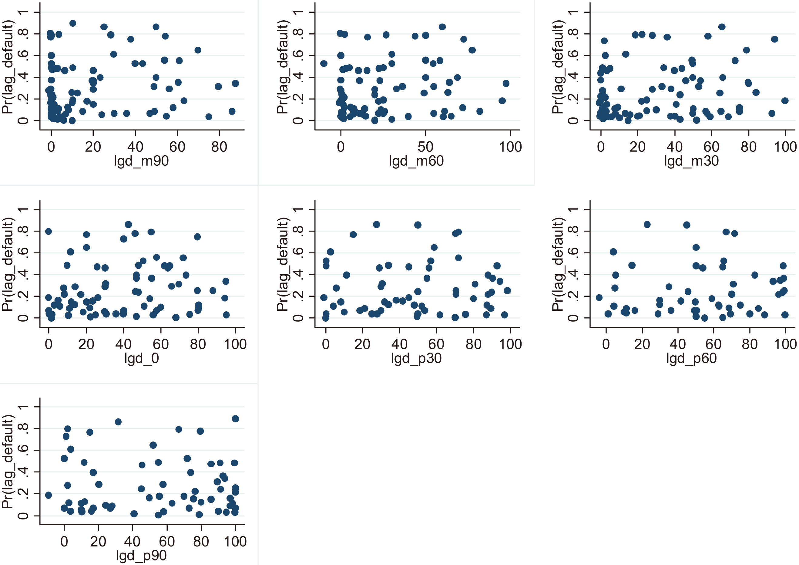

Table 11

Observed default rates and recovery rates

	Total value	Total value of	Default rate (1)	The total	The number	Default rate (2)	LGD at	LGD	LGD	LGD
Year	of emissions,	outstanding	by the volume	number	of defaulted	by the share of	the moment	( $+$	( $+$	( $+$
	bln. rub.	commitments,	of emissions	of emitters	emitters	defaulted emitters	of default	30 days)	60 days)	90 days)
		bln. rub.
2014	6,623.01	6.54	0.10%	359.00	13.00	3.62%	18.32	40.34	38.91	41.67
2013	5,189.32	9.26	0.18%	353.00	11.00	3.12%	36.80	89.45	85.00	96.98
2012	4,165.75	2.20	0.05%	342.00	6.00	1.75%	7.97	5.50	4.83	1.98
2011	3,436.58	6.57	0.19%	349.00	25.00	7.16%
2010	2,965.43	59.53	2.01%	394.00	74.00	18.78%	28.50	30.22	25.80	37.45
2009	2,568.75	132.58	5.16%	440.00	119.00	27.05%	44.19	46.84	54.20	51.66
2008	1,814.99	37.88	2.09%	495.00	54.00	10.91%	34.19	52.87	64.23	62.57
2007	1,272.04	2.05	0.16%	487.00	3.00	0.62%	–	–	–	–
2006	905.62	0.40	0.04%	391.00	1.00	0.26%	–	–	–	–
2005	481.26	0.01	0.00%	253.00	1.00	0.40%	50.00	–	–	50.00
2004	263.35	0.07	0.03%	189.00	3.00	1.59%	24.42	50.00	50.00	50.00
2003	159.51	–	0.00%	162.00	1.00	0.62%	–	–	–	–
2002	112.32	0.05	0.04%	108.00	1.00	0.93%	–	–	–	–

Note: the empty cells in the table mean that there are no defaults in the year, or LGD cannot be observed due to the lack of bond trading.

Fig. 6.

PD&LGD relationship based on results of PD model: out of time.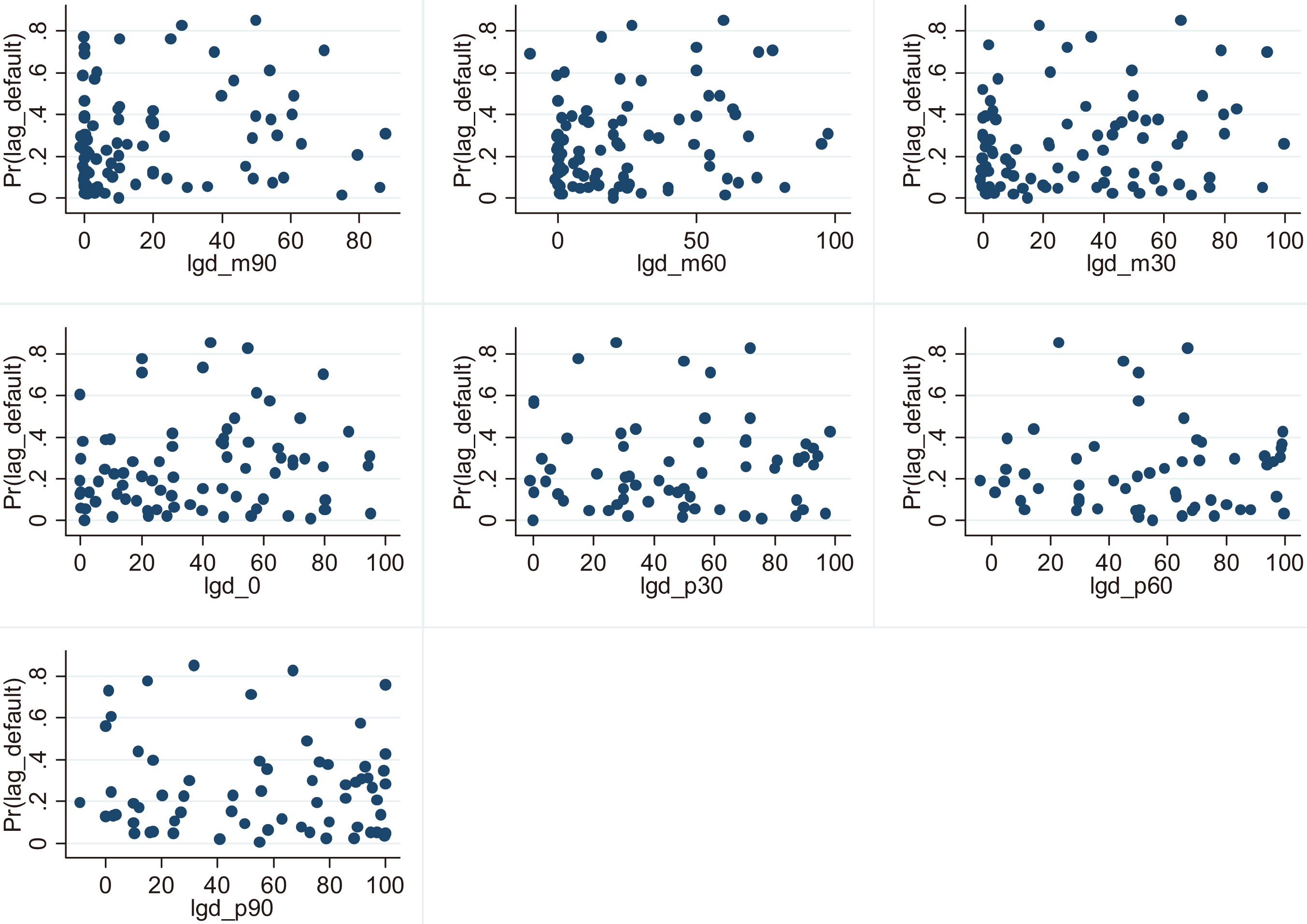

6. PD & LGD correlation

6.1 PD & LGD correlation based on estimated PD and observed recovery rate

In this Section PD&LGD correlation based at borrower level is described.

The best PD model was recognized the model with higher accuracy (R2) and discriminatory power from each two attempts (out-of-sample, out-of-time).

PD is estimated for bond issuer $i$ in year $t$ . LGD is estimated for bond $j$ in year $t$ .

Example:

•
Bond ‘A’ default occurs 01.09.2010.
•
LGD rate is the price of Bond ‘A’ in 30 days (01.10.2010) divided by the bond face value. We also examine the bond price in 30, 60, 90 days before and after default, and in the event of default as proxies for LGD.
•
PD is estimated for Bond ‘A’ issuer using the annual financial statements of 2009 to predict PD for one year.
•
PD-LGD correlation was found using PDs and LGDs of all default bonds over the sample period if there are available financial statements of bond issuers and available bond prices.

Fig. 7.
Different representation of correlation between PD and LGD.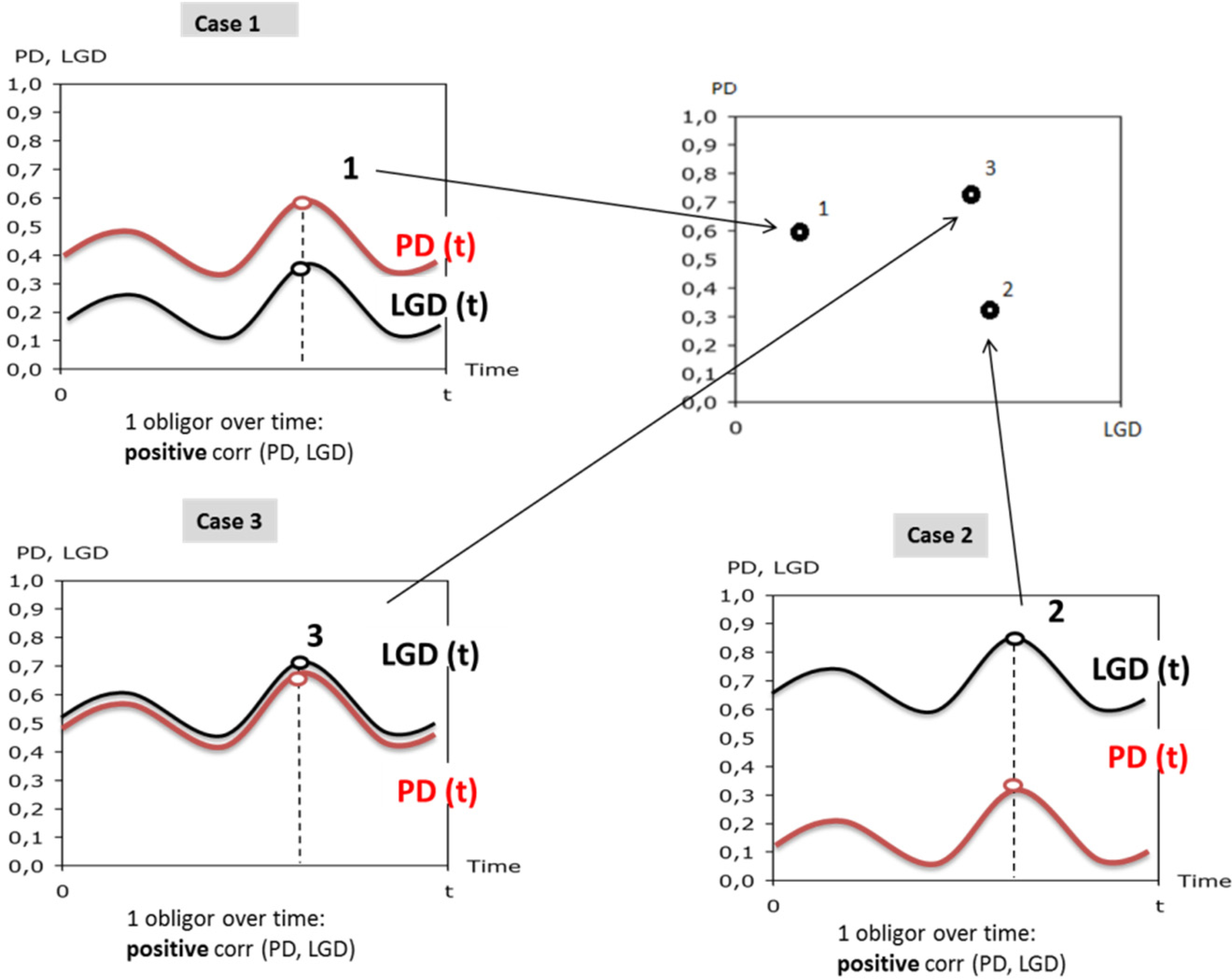

A correlation matrix was constructed (Table 10) to show that the result is stable under the different models. The relationship between PDs and LGDs is small. The link become weaker after default, however it may be in response with numbers of observations (the problem was discussed in the Section 3).

As it can be seen from the graphs above, the relationship between the probability of default and the recovery rate is not visually evident. It means that the PD-LGD correlation is zero. This conclusion is not consistent with the results of previous works. The different results could be obtained because of different methodologies. The correlation was estimated using estimates of PD and LGD for different borrowers for whom defaults occurred in different years instead annual market PDs and LGDs per year.

The conclusion about the lack of correlation between PD and LGD does not mean that the correlation between PD and LGD do not exist. The example is shown in Fig. 7. Using the approach selected for this study, we saw the result based on PD and LGD for different borrowers with different years of default. However, this observation is only the case at a particular point in time, i.e. it is the point of the time series, which may reflect the relationship between PD and LGD for some period. Therefore, we can observe the correlation between PD and LGD on each graph with time series, but we cannot see this correlation on the graph with vertical axis PD and horizontal axis LGD.

Miu and Ozdemir, (2005) noted that the PD-LGD correlation could be not only positive because of lagging dependence, i.e. the cycle of recovery rate varies with PD cycle. This case could be explained by the fact that both parameters are affected by various factors, including different macroeconomic factors.

Fig. 8.
Relationship between PD and LGD at the moment of default. Case 1: default rate by volume of emissions.

Fig. 9.
Relationship between PD and LGD at the moment of default. Case 2: default rate by the number of defaulted emitters.

Fig. 10.
Relationship between PD and LGD in 30 days after default. Case 1: default rate by volume of emissions.

Fig. 11.
Relationship between PD and LGD in 30 days after default. Case 2: default rate by the number of defaulted emitters .

Fig. 12.
Relationship between PD and LGD in 60 days after default. Case 1: default rate by volume of emissions.

Fig. 13.
Relationship between PD and LGD in 60 days after default. Case 2: default rate by the number of defaulted emitters.

Fig. 14.
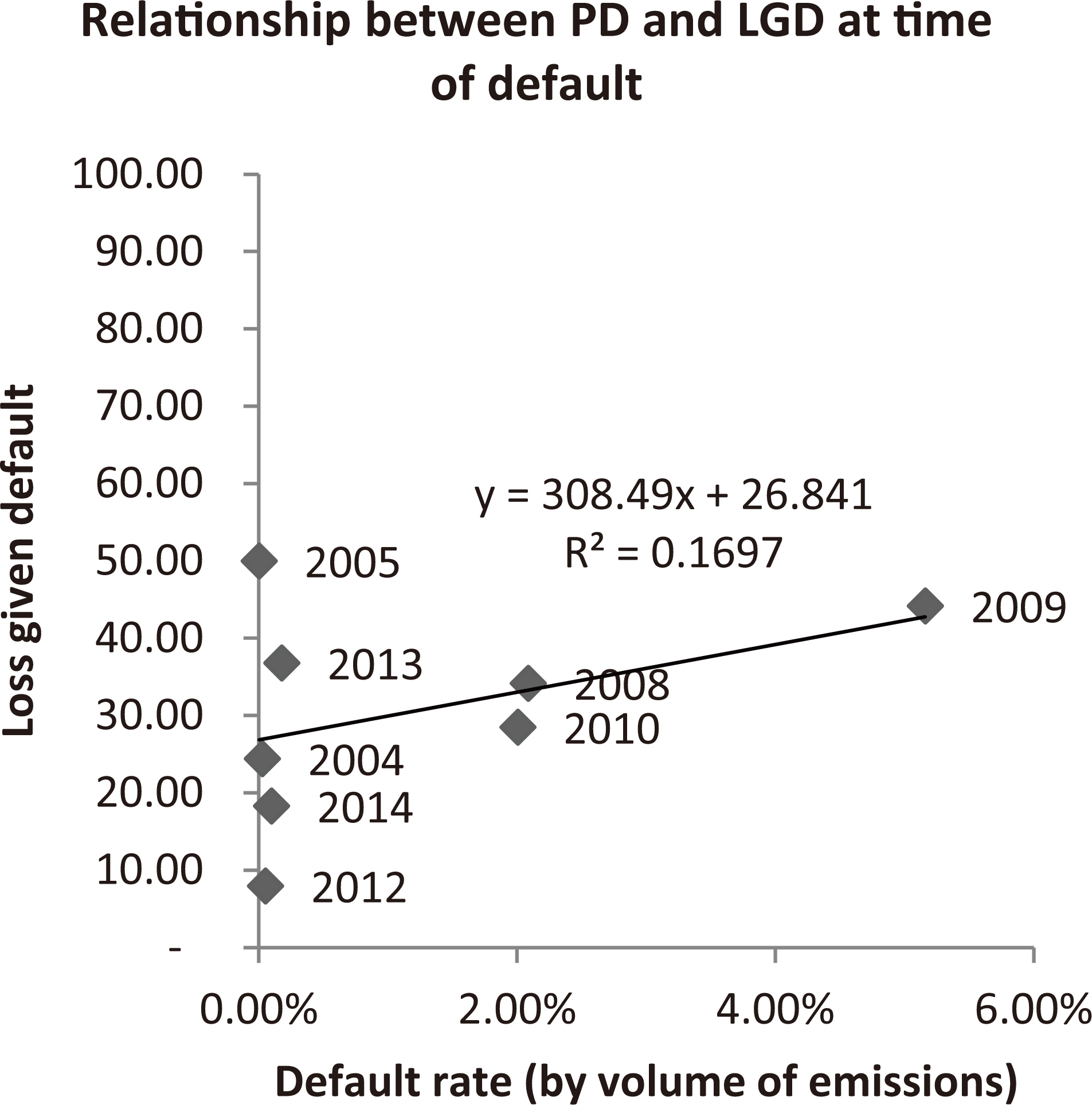
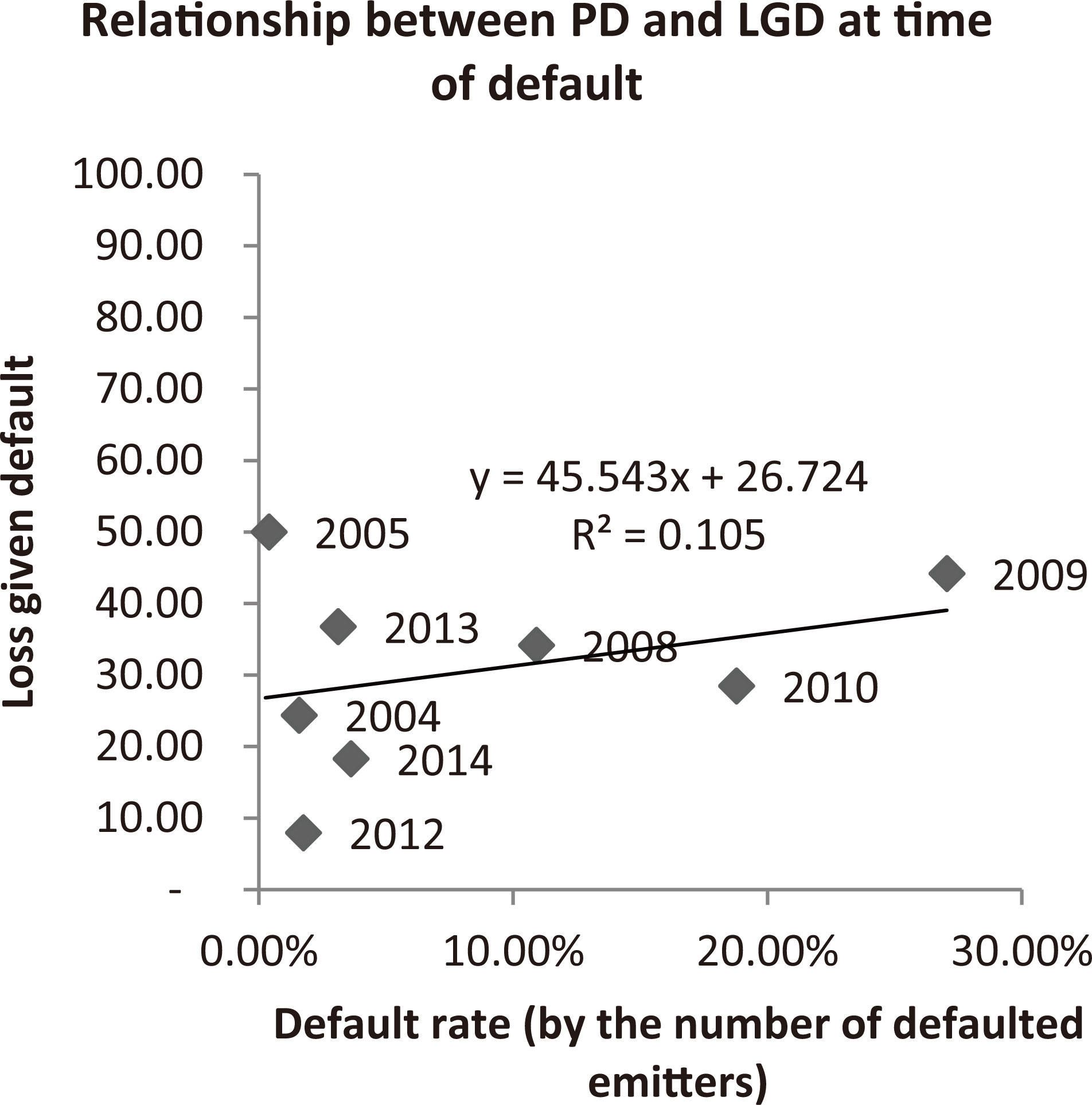
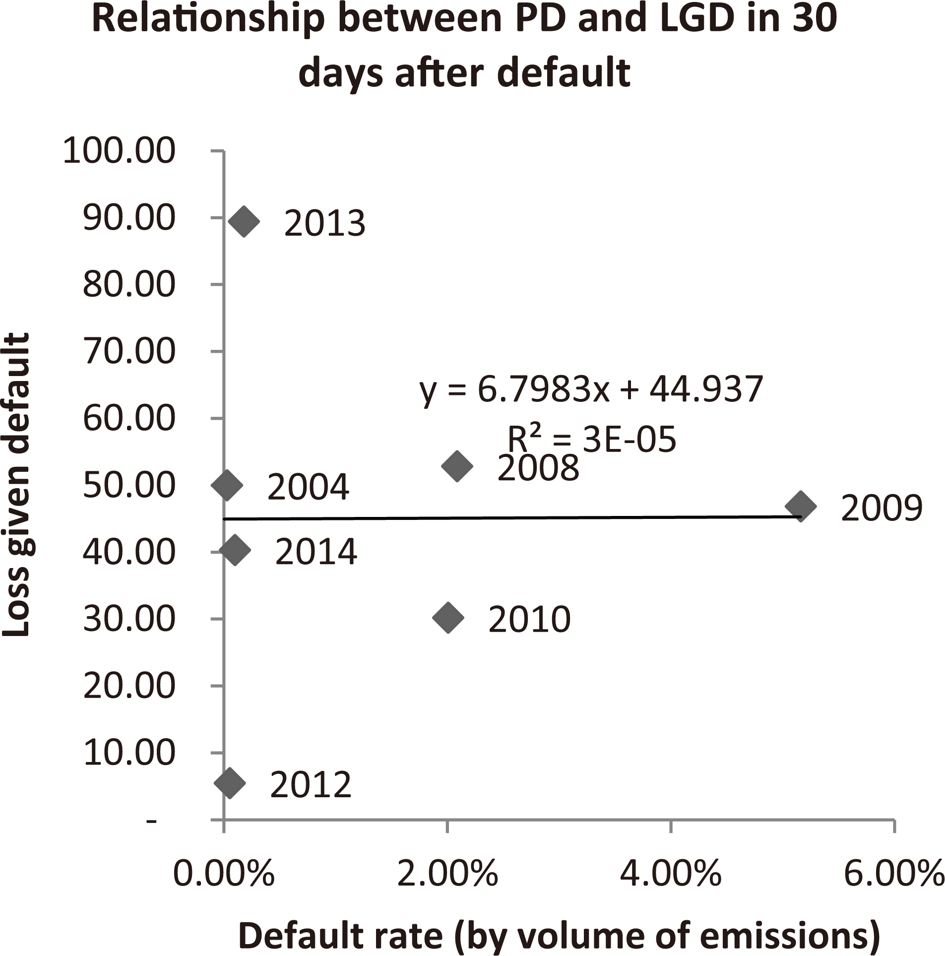
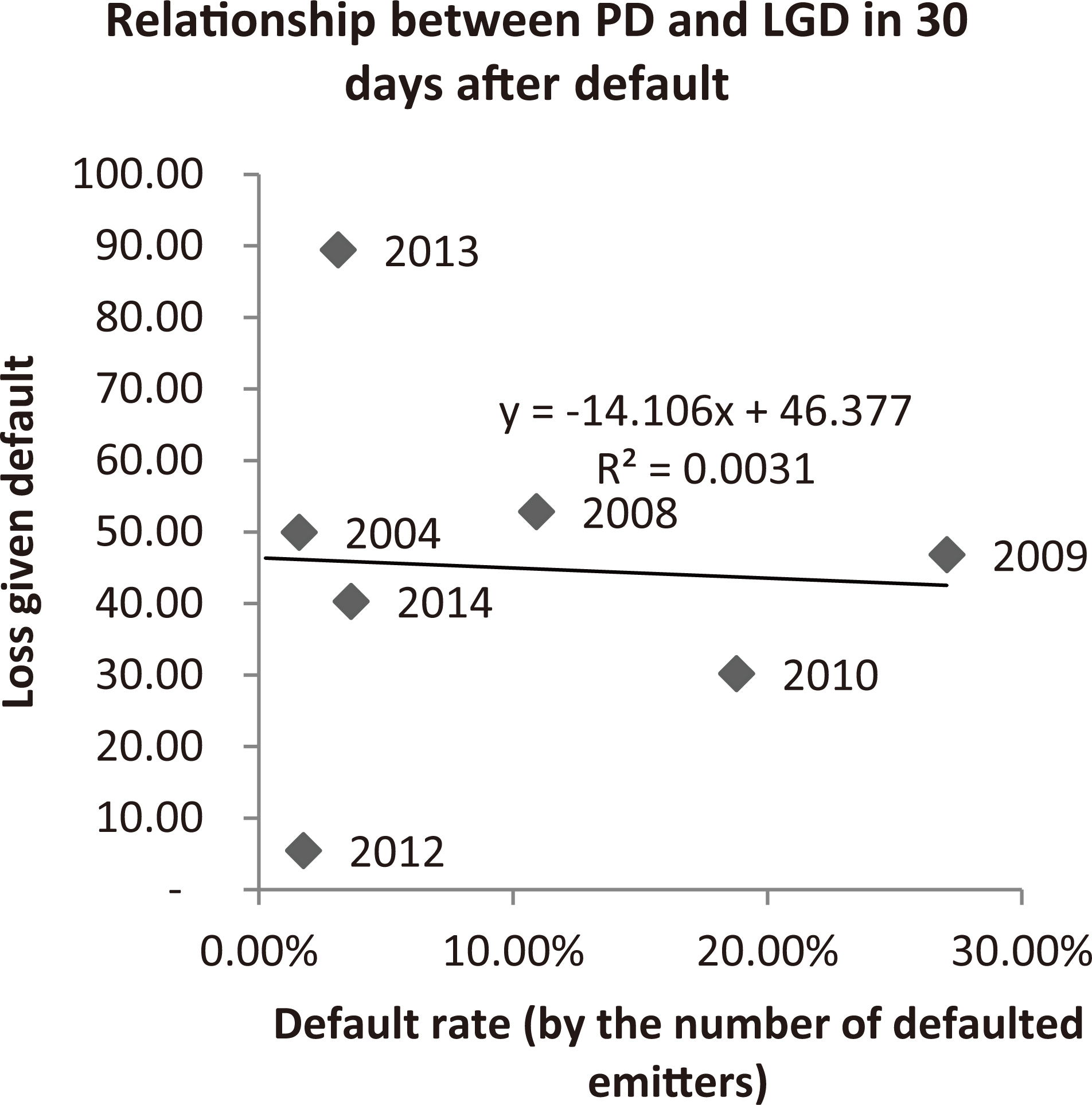
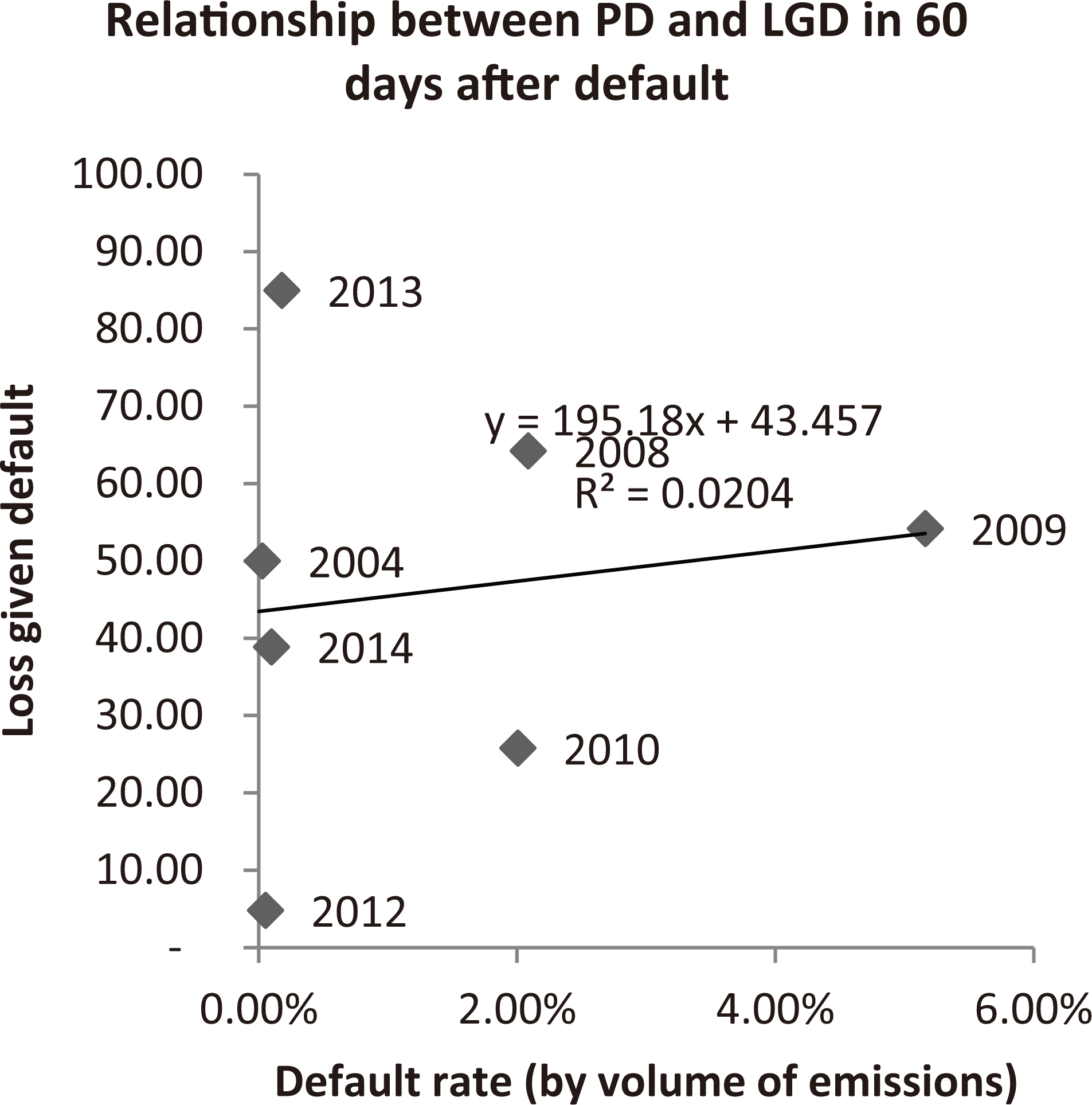
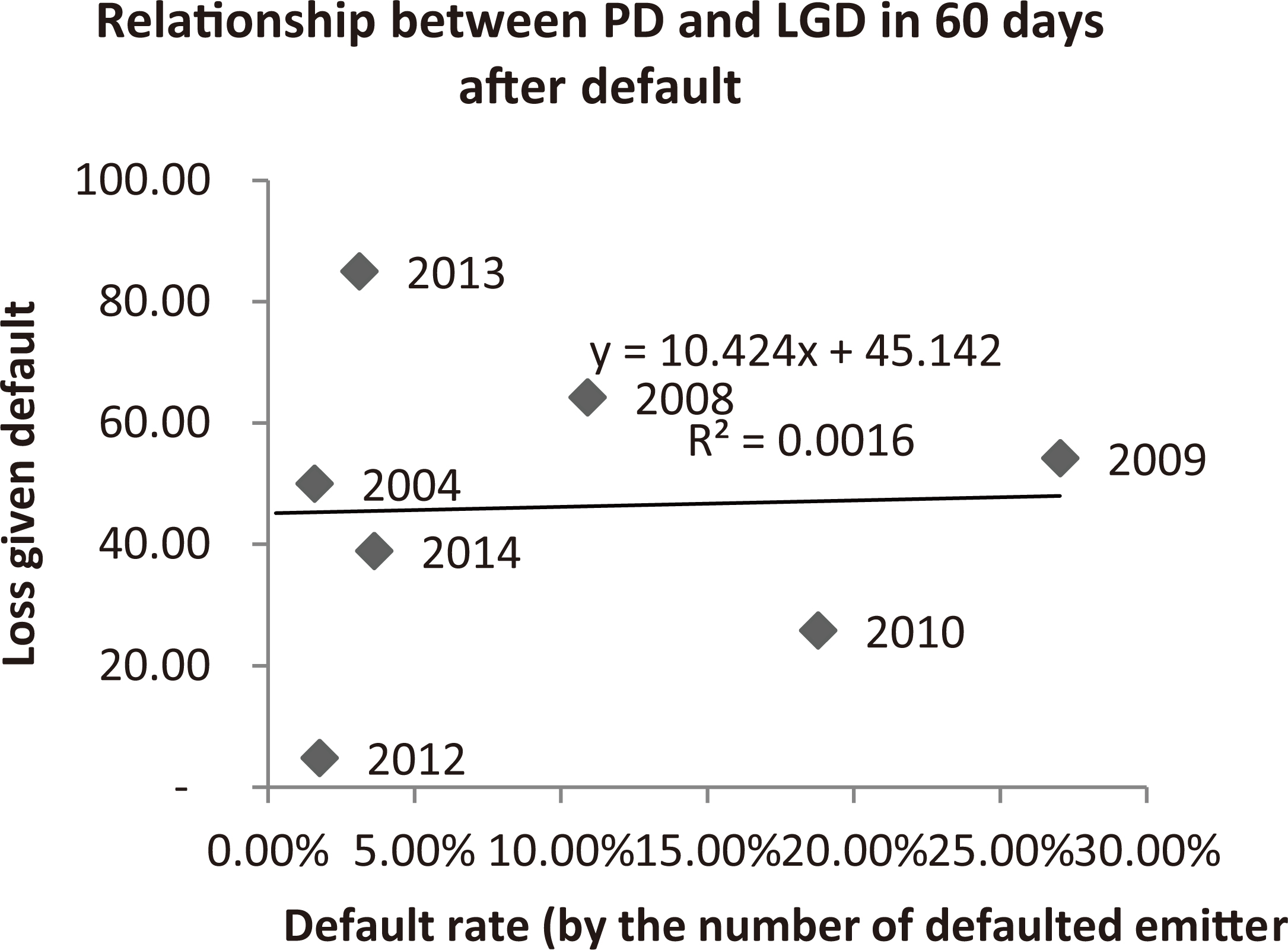
Relationship between PD and LGD in 90 days after default. Case 1: default rate by volume of emissions.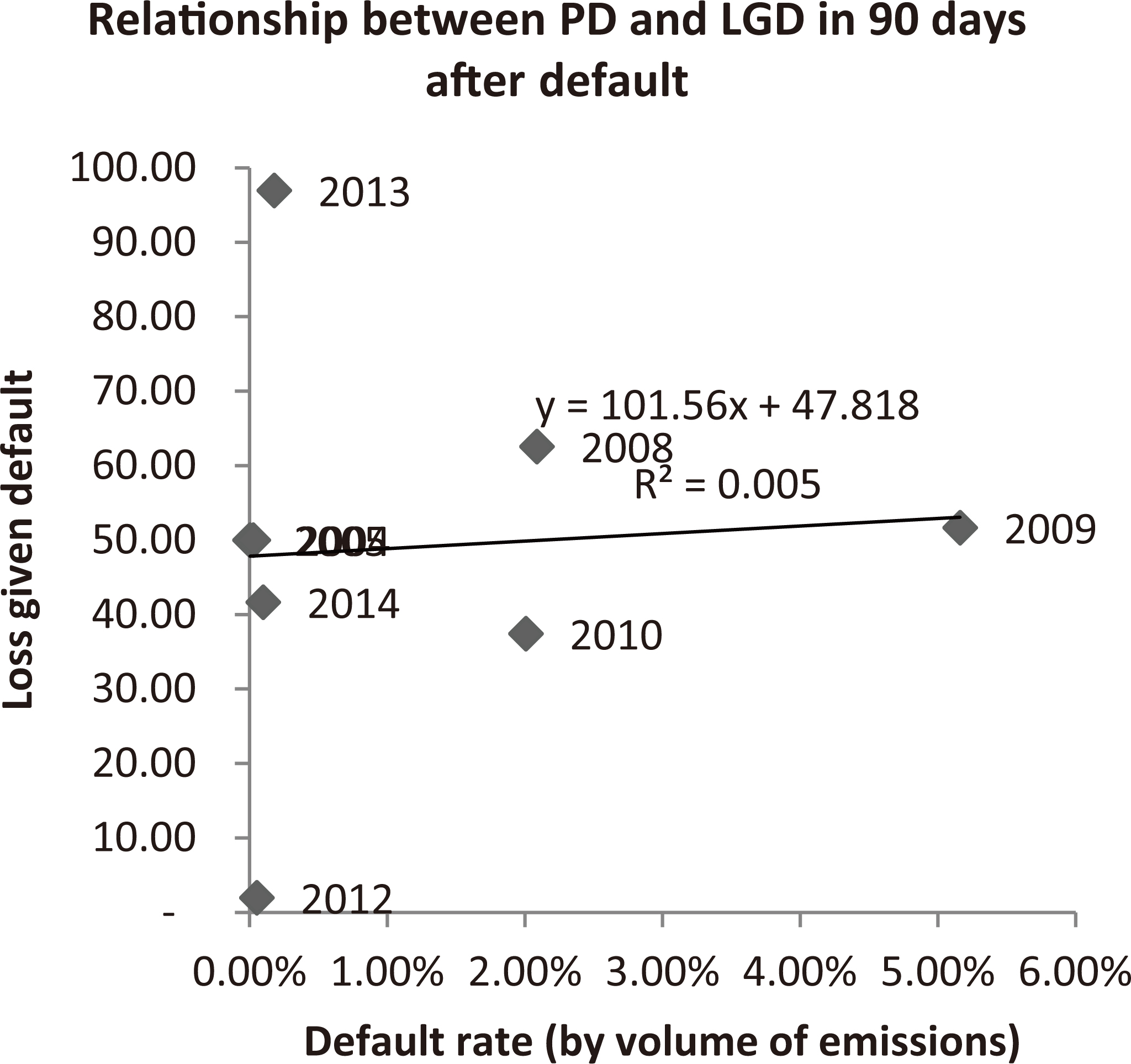

Fig. 15.
Relationship between PD and LGD in 90 days after default. Case 2: default rate by the number of defaulted emitters.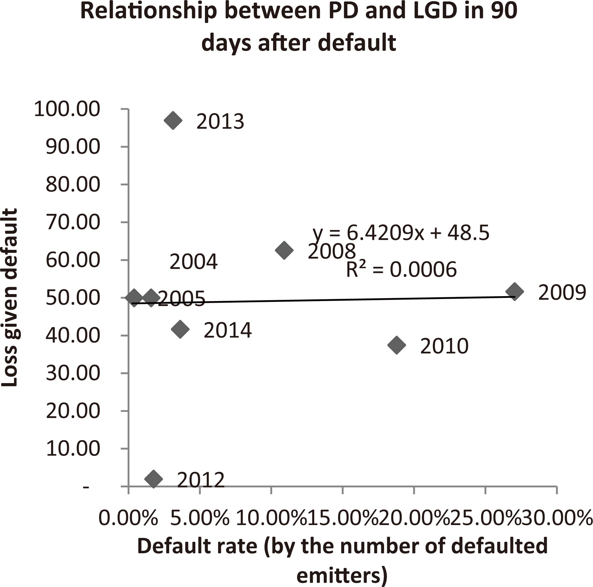

As we discussed earlier, LGD can be underestimated if a bond price remains unchanged after default (ending the bond trade on the exchange). The bond price, which is a key factor in assessing the recovery rate by the market-based approach, may be overstated for a financial instrument due to its illiquidity. In other words, at some point of trades bond turnover stops and the price remains at a level, this does not correspond to the actual level of recoveries. Such cases were found companies in the examined sample. Thus, evaluation of the relationship between PD and RR (or LGD) requires the inclusion liquidity in the model. Perhaps in emerging markets, it should be considered as changes in the volume of transactions regarding the cost ( $\mathrm{\Delta P*V}$ ).
6.2 PD & LGD correlation based on observed default rate and recovery rate

The US data is covered about 20 years, while the Russian data covers only the eight points. Therefore, we decided not to study the correlation using average market PD and LGD per year. However, in this section we present Figs 8–15 to show the result that we could take if we apply the same methodology as for the US data in the previous works.

The default rates are calculated in two ways: by volume of emissions and by the number of defaulted emitters. The first approach determines a default rate as the ratio between outstanding commitments and total value of emissions on corporate bond market. The second way defines a default rate as the number of defaulted emitters to the total number of bond issuers.

The analysis also shows that there is no the PD-LGD correlation for the Russian market. For example, in the study (Altman, 2005) the relationship between PD and LGD is determined at the time of default building regression, where the proportion of predicted variance reached 51% at linear regression and 65% for a quadratic. In our case the maximum proportion of predicted variance does not exceed 17% and even more the regression line has a positive slope supported by three points that relate to years of the most severe recession (2008–2010).

The authors of Altman (2005) explained the phenomenon of positive correlation between PD & LGD as the increase in bond supply before its default, that decrease a price of bond that soon to became defaulted, consequently, decrease recovery rate, and the opposite increase LGD. This trend can be observed in the Russian corporate market too but not always (see the dynamics of bond prices in Table 14).

Thus, the results about the lack of correlation between PD and LGD are confirmed on observed default rates and LGD.

7. Conclusion

The mainstream of risk-management research focuses on analysis on PD-LGD correlation. It should originated from the fact that the more likely the borrower is not pay back on its debt, the more likely the recovered amount is small. Papers based on developed countries provide findings that PD and LGD are not independent due to systematic risk factor. Positive correlation between PD and LGD (or, equally, negative correlation between PD and recovery rate) is the most frequent result of previous research. However, this research cannot argue that there is positive PD-LGD dependence for Russian corporate borrowers. The methodology of work is different from earlier works. The relationship is estimated on a sample of different borrowers with different years of default, i.e. on obligor-level but not on year-level where each observation presents a ratio of PD and LGD for year.

Thus, the evidence is that using Russian data one cannot argue for the presence of risk parameter dependence whereas research using developed countries’ data suggests there is a positive one. The implication would be that there is no need to overcharge capital for Russian banks compared to their counterparts from developed countries.

Footnotes

The Basel Committee was founded in 1974 to set standards of banking supervision. As of August 2017, the Basel Committee comprises 28 jurisdictions including developed and developing countries.

The Basel standards differentiate LGD only between secured (LGD $=$ 45%) and unsecured (LGD $=$ 75%) loans. Please, see par. 287–288 of Basel II (2006) for more details. URL: http://www.bis.org/publ/bcbs128.pdf.

Please, see par. 472 of Basel II (2006) for more details. URL: http://www.bis.org/publ/bcbs128.pdf.

Russia published first drafts of the regulation in 2012 (for example, CBR letter No. 192-T about Internal Rating-Based Approach).

Developed countries: Australia, Hong Kong SAR, Saudi Arabia, and Singapore. Developing countries: Argentina, Brazil, China, India, Indonesia, Korea, Mexico, Russia, South Africa, Turkey.

Example: Suppose risk-weighted assets $=$ 100$. Then capital $=$ 100$ * 8% $=$ 8$ (according to the Basel standards). Taking into account PD-LGD correlation, capital should be 8$ * 1.4513 $=$ 11.6$ (1.4513 is Moodys (2010) estimates of the capital shortfall). Then the minimum capital requirements should be 11.6% to ensure 11.6$ of capital. The Basel Committee needs to increase the capital requirements by 1.1 percentage points: 8% (minimum total capital requirements) $+$ 2.5% (capital conservation buffer) $+$ 1.1% (capital add-on to cover PD-LGD correlation risk fully according to Moody’s estimates) $=$ 11.6%.

The Basel Committee reflects the national discretions in the document at http://www.bis.org/bcbs/publ/d297.pdf.

Correlation between parameters was also assessed on retail data (Witzany, 2011).

Acknowledgments

The paper is prepared within the Fundamental Research Program of the National Research University Higher School of Economics (NRU HSE) with the use of the state subsidy ‘5-100’ program for the leading universities of the Russian Federation. Any opinions or claims contained in this research do not necessarily reflect the views of Higher School of Economics. We thank the anonymous reviewers for many insightful comments.

Appendix

References

Altman

E. I.

(2006). Default recovery rates and LGD in credit risk modeling and practice: An updated review of the literature and empirical evidence. New York University, Stern School of Business.

Altman

E. I.

, et al., (2005). The link between default and recovery rates: Theory, empirical evidence, and implications. The Journal of Business, 78(6), 2203-2228.

Altman

E. I.

(1968). Financial ratios, discriminant analysis and the prediction of corporate bankruptcy. The Journal of Finance, 23(4), 589-609.

Antonova

(2013). The estimation of recovery rate for corporate bonds of Russian issuers. Ph.D. Thesis. Higher School of Economics, Moscow, Russia.

Araten

Jacobs

, & Varshney

(May 2004). Measuring LGD on commercial loans: An 18-year internal study. RMA Journal, 86(8), 96-103. (цит. по Miu

, & Ozdemir

(2006). Basel Requirement of Downturn LGD: Modeling and Estimating PD & LGD Correlations. Journal of Credit Risk2(2)).

Backshall

Giesecke

, & Goldberg

(2004). Credit risk modeling. Handbook of Fixed Income Securities, Wiley.

Bandyopadhyay

(2006). Predicting probability of default of Indian corporate bonds: Logistic and Z-score model approaches. Journal of Risk Finance, 7(3), 255-272.

Basel Committee on Banking Supervision, (October 2001). Working paper on the internal ratings-based approach to specialised lending exposures, BIS.

Basel Committee on Banking Supervision, (June 2004). International convergence of capital measurement and capital standards, BIS.

10.

Bhatia

(2006). Credit risk management and Basel II – an implementation guideline. London: Risk Books.

11.

Cameron

A. C.

, & Trivedi

P. K.

(2005). Microeconometrics: Methods and applications. New York: Cambridge University Press.

12.

Carey

, & Michael

(2003). Systematic risk in recoveries on defaulted debt. mimeo, Federal Reserve Board, Washington. (citation by Altman

E. I.

, et al., (2005). The Link between default and recovery rates: Theory, empirical evidence, and implications. The Journal of Business, 78(6), 2203-2228).

13.

Chava

Stefanescu

, & Turnbull

(2011). Modeling the loss distribution. Management Science, 57(7), 1267-1287.

14.

Düllmann

, & Trapp

(2004). Systematic risk in recovery rates – an empirical analysis of US corporate credit exposures. EFMA 2004 Basel Meetings Paper.

15.

Dwyer

Korebleva

, & Dzhao

(2010). RiskCalc model v3.1. for Russian companies. Modeling Methodology, Moody’s KMV.

16.

Frye

(Sep 2000). Collateral damage detected. Emerging Issues.

17.

Frye

(2000). Depressing recoveries. Risk London Risk Magazine Limited, 13(11), 108-111.

18.

Giese

(2005). The impact of PD/LGD correlations on credit risk capital. Risk London Risk Magazine Limited, 18(4), 79.

19.

Gupton

, & Stein

(2002). LossCalc: Model for predicting loss given default (LGD). Moody’s Investors Service.

20.

Y. T.

, & Perraudin

(2002). The dependence of recovery rates and defaults. Birbeck College and Bank of England, Working Paper.

21.

Jarrow

(2001). Default parameter estimation using market prices. Financial Analysts Journal, 57(5), 75-92.

22.

Jokivuolle

, & Peura

(2003). Incorporating collateral value uncertainty in loss given default estimates and loan-to-value ratios. European Financial Management, 9(3), 299-314. (citation by Altman

E. I.

, et al., (2005). The link between default and recovery rates: Theory, empirical evidence, and implications. The Journal of Business, 78(6), 2203-2228.

23.

Letter from the Bank of Russia. (29 December 2012). About methodological recommendations on the implementation of the approach to the calculation of the credit risk on the basis of internal ratings of banks. (192).

24.

Madan

D. B.

Bakshi

, & Zhang

F. X.

(2006). Understanding the role of recovery in default risk models: Empirical comparisons and implied recovery rates. (citation by Altman

E. I.

, et al., (2005). The Link between default and recovery rates: Theory, empirical evidence, and implications. The Journal of Business, 78(6), 2203-2228).

25.

Meng

, et al., (2010). Implications of PD-LGD correlation in a portfolio setting. Moody’s Analytics. http://www.moodysanalytics.com/∼/media/Insight/Quantitative-Research/Portfolio-Modeling/10-05-02-Implications-of-PD-LGD-Correlation-in-a-Portfolio-Setting.ashx [18.01.2015; free access].

26.

Miu

, & Ozdemir

(2006). Basel requirement of downturn LGD: Modeling and estimating PD & LGD correlations. Journal of Credit Risk, 2(2), 43-68.

27.

Ohlson

J. A.

(1980). Financial ratios and the probabilistic prediction of bankruptcy. Journal of Accounting Research, 18(1), 109-131.

28.

Resolution of the FAS of Far East District from 02.12.2013 N F03-5071 / 2013 in the case N A73-7131 / 2010 Basel Committee on Banking Supervision, (June 2004). International Convergence of Capital Measurement and Capital Standards, BIS.

29.

Seidler

(2008). Implied market loss given default: Structural-model approach (No. 26/2008). IES Working Paper.

30.

Thesis of Bank of Russia. (28 December 2012). About the method of determining the value of own funds (capital) of credit institutions. 395-P.

31.

Totmjanina

(2011). Evaluation of the probability of default for industrial companies on the basis of financial indicators. Finansovyj Menedzhment (Russian transliteration), 11(53), 59-68.

32.

Totmjanina

(2011). Overview of default probability models. Upravlenie Finansovymi Riskami (Russian transliteration), 1(25), 12-24.

33.

Vasicek

(1987). Probability of loss on loan portfolio. KMV Corporation, 12(6).

34.

Witzany

(2011). A two factor model for PD and LGD correlation. Bulletin of the Czech Econometric Society, 18(28).

PD-LGD correlation study: Evidence from the Russian corporate bond market

Abstract

Keywords

1. Introduction

2. Literature review

3.1 Data for PD estimates

Table 1 The distribution of defaulted and non-defaulted companies in both initial and final samples.9 9 As comparison with the previous version of research the sample was expanded by 2642 observations having panel data structure.

Table 3 The descriptive statistics of recovery rates based on bond prices

Table 5 The stages of PD model development (out-of-sample)

Table 9 Regression output: pool regression and regression with random effect

Table 10 Correlation matrix: Pearson correlation between LGDs and PDs from different models

6.1 PD & LGD correlation based on estimated PD and observed recovery rate

7. Conclusion

Footnotes

Acknowledgments

Appendix

References

Table 1
The distribution of defaulted and non-defaulted companies in both initial and final samples.9
⁹
As comparison with the previous version of research the sample was expanded by 2642 observations having panel data structure.

Table 3
The descriptive statistics of recovery rates based on bond prices

Table 5
The stages of PD model development (out-of-sample)

Table 9
Regression output: pool regression and regression with random effect

Table 10
Correlation matrix: Pearson correlation between LGDs and PDs from different models