Investigating effects of bandwidth selection in local polynomial regression model with applications

Abstract

Cross-validation (CV) and direct plug-in (DPI) are two commonly used bandwidth selection methods in nonparametric estimation. In this paper, we compare the performance of CV and DPI methods in local polynomial kernel regression through simulation study. We consider continuous response and binary response cases, with local constant, local linear and local quadratic kernel estimators, respectively. Furthermore, we investigate the first derivatives of local quadratic kernel estimators. Our results show that CV and DPI methods excel in different cases, in terms of minimizing the Mean Integrated Squared Errors (MISE); the results are also verified in empirical studies.

Keywords

Cross-validation directly plug-in method first-order derivative generalized linear model local polynomial estimator

1. Introduction

Local polynomial kernel regression is a widely used nonparametric smoothing approach, by which the pointwise estimation of the curve only depends on observations in a neighborhood of a to-be-determined radius (e.g., Woolhouse, 1870; Stone, 1977; Loader, 1996; Cleveland & Loader, 1996). There is a vast literature on choosing the radius, also known as the bandwidth selection problem. For example, the literature on local polynomial regression, where the pointwise estimate is given by a polynomial of a fixed and given order, has much discussion on bandwidth selection criteria, order of local polynomials, comparison among different selection methods, small and large sample properties of the estimators.

Essentially, the bandwidth acts as a smoothing parameter, balancing the bias-variance trade-off. Under a small bandwidth, the fitting curve is relatively volatile but follows the observations closely; under a large bandwidth, the fitting curve is relatively smooth, while the estimation bias is relatively large. An estimator will perform poorly with respect to the bandwidth near the boundaries of the data if a kernel density estimation is employed, particularly when the underlying density has long tails (Zambom & Dias, 2012). On the other hand, the specification of the local polynomials contributes to the curve estimation through the order of polynomial (Xia & Li, 2002; Li & Racine, 2007). Xia and Li (2002) stated that higher-order polynomial produces robust estimates for the optimal bandwidth, but only in a large sample; Li and Racine (2007) also mentioned that by using higher-order polynomial fitting, the estimation bias is reduced without any increase in the Mean Squared Error (MSE). Altogether, the selection of the bandwidth and the polynomial orders form a crucial part of the specification for a local polynomial kernel regression problem, and a nonparametric approach can be very powerful for estimating the mean functions and its derivatives (Fan & Gijbels, 1995).

In the context of bandwidth selection methods, a common optimization objective is Mean Integrated Squared Errors (MISE) where the minimizer is the theoretical optimal bandwidth (e.g., Fan & Gijbels, 1992; Li & Racine, 2007; Ruppert et al., 1995; Xia & Li, 2002). We can estimate MISE by replacing the unknown integrals in the expression of the MISE-minimizer with the estimators, which is the basic idea of a plug-in method (Li & Racine, 2007; Ruppert et al., 1995), or by utilizing a cross-validation (CV) method (Bowman, 1984; Li & Racine, 2007; Rudemo, 1982). The CV method provides a fully-automatic data-driven approach, while the performance of plug-in methods heavily depends on the pilot bandwidth specification. Further, the CV method reacts to the uncertainty of bandwidth selection by under-smoothing, while plug-in methods react by over-smoothing (Loader, 1999). The CV-selected bandwidth’s tendency to under-smooth can cause a downward bias and a lack of robustness in the estimators of derivatives (Newell & Einbeck, 2007). On the other hand, the plug-in method can asymptotically result in inefficient estimates due to its difficulties in efficiently using curvature information (Loader, 1999).

There are different types of plug-in bandwidth estimators, including the rule of thumb (ROT), direct plug-in (DPI) and solve the equation (STE); one of these “plug-in” bandwidth estimators, the DPI estimator, outperforms the others in the majority of cases in terms of converging to the MISE-optimal bandwidth (Ruppert et al., 1995). Wand and Jones (1994) discussed the performance of MISE- and DPI-bandwidth estimators for the density estimation. However, there has not been much discussion directly on the comparison between the two bandwidth selection approaches for local polynomial kernel regression in the literature. Hence, in this article, we compare the performance of CV and DPI methods for local polynomial kernel regression in both continuous response and binary response cases through both simulation and empirical studies.

When the response is continuous, not only can we do analysis and inference on the level functions but also on its derivatives for local polynomial kernel estimators of sufficient order. Fan and Gijbels (1996) suggested that assuming existence, to estimate the $k^{th}$ order derivatives, one should use an order- $p$ polynomial, such that $k<p$ and $p-k$ is an odd number. Hence, in this article, we compare the performance of polynomials with order 0 to 2 (i.e., local constant, local linear and local quadratic kernel estimators, respectively).

Finally, Song et al., (2006) proposed to apply the function dpill() in R package to obtain the bandwidth for the local quadratic estimator and the first derivative of the function. As we have known, dpill() is only suitable to the local linear estimator. Therefore, based on this motivation, we also investigate the bandwidth selection methods for the first-order derivative. In essence, we estimate the first order derivatives using local quadratic kernel estimators. Our results show that CV and DPI methods selection methods excel in different cases; the results are also verified in empirical studies. Specifically, we find that results generated from the binary response case are not consistent with the results from the continuous response case. Furthermore, DPI is consistently better at identifying local maxima by estimating the first derivatives in a local quadratic kernel setting.

The remainder of this article is structured as follows: in Section 2, we will briefly introduce the bandwidth selection and estimation procedures of local polynomial kernel estimators for classic and generalized linear models. Section 3 presents the simulation study with the first three orders of the local polynomial case by case. We present the analysis of three different real data in Section 4. Finally, we will discuss and conclude our findings in Section 5.

2. Estimation procedure

In this section, we will briefly review local polynomial kernel estimation and bandwidth selection for a continuous response, of which the details are presented in Fan and Gijbels (1996). Afterward, we introduce the corresponding extension to a binary response case.

First, note that there are two unknowns in local polynomial kernel estimation – the bandwidth $h$ and the kernel function $K_{h}(\cdot)$ for a given $h$ . Since we focus on the relative comparison between CV- and DPI-bandwidth estimators, we will only consider a Gaussian kernel in the current paper. To justify this, it has been noted in the literature that the choice of kernel functions has less significant effects on the estimators as opposed to the bandwidth (Wand & Jones 1994, p. 31). Furthermore, we mainly examine the relevant continuous covariates.

2.1 Continuous response

Consider a model specified as follows:

$\displaystyle y_{i}=m(x_{i})+\epsilon_{i},\quad\forall i=1,\ldots,n,$ (1)

where $\epsilon_{i}$ is i.i.d., as such $E(\epsilon_{i})=$ 0 and $\text{Var}(\epsilon_{i})=\sigma^{2}$ . Our goal is to estimate the function $m(\cdot)$ or its order- $p$ derivative $m^{(p)}(\cdot)$ . For a fixed $x$ , if $m(x)$ is smooth at $x$ , then by Taylor expansion,

$\displaystyle m(u)\approx m^{(0)}(x)+m^{(1)}(x)(u-x)+\ldots+\frac{m^{(p)}(x)}{% p!}(u-x)^{p}.$ (2)

Defining $\beta_{0}=m^{(0)}(x)=m(x)$ , $\beta_{1}=m^{(1)}(x)$ , $\ldots$ , $\beta_{p}=\frac{m^{(p)}(x)}{p!}$ , for $j=0,\ldots,p$ , it suffices to estimate the $\beta_{j}$ ’s for estimating different orders of derivatives of the function $m(\cdot)$ (considering the level function for the zero-order derivative). We can obtain the least square estimators by minimizing the weighted sum of squared errors with the kernel function $K_{h}(\cdot)$ (Fan & Gijbels, 1996), such that

$\displaystyle\left(\hat{\beta}_{0},\hat{\beta}_{1},\ldots,\hat{\beta}_{p}% \right):=\operatorname*{argmin}\limits_{\left({\beta}_{0},{\beta}_{1},\ldots,{% \beta}_{p}\right)}\sum\limits_{i=1}^{n}K_{h}\left(\frac{x_{i}-x}{h}\right)% \left[y_{i}-\beta_{0}-\beta_{1}(x_{i}-x)-\ldots-\beta_{p}(x_{i}-x)^{p}\right]^% {2}.$ (3)

As mentioned earlier, we will show the estimations of $m^{(0)}(x)$ and $m^{(1)}(x)$ using $p=$ 0, $p=$ 1 and $p=$ 2, where the estimate of $m^{(1)}(x)$ can be obtained in the $p=$ 2 case. In particular, if $p=$ 0, we can obtain a local constant kernel estimator, $\hat{\beta}_{0}$ , also known as the Nadaraya-Waston estimator; if $p=$ 1, we can obtain local linear kernel estimators, $\hat{\beta}_{0}$ and $\hat{\beta}_{1}$ ; if $p=$ 2, we can obtain local quadratic kernel estimators, $\hat{\beta}_{0}$ , $\hat{\beta}_{1}$ and $\hat{\beta}_{2}$ . For $p=$ 0 and $p=$ 1, we are interested in the estimation of the level function, which is $\hat{\beta}_{0}$ , and for $p=$ 2, we are interested in the estimation of both the level function and the first order derivative, which are $\hat{\beta}_{0}$ and $\hat{\beta}_{1}$ .

With the orders of polynomials determined, we now consider the bandwidth selection. The idea behind the CV method is to optimize the out of sample performance of the estimator by minimizing the leave-one-out sum of squared error (SSE). Specifically, to obtain the leave-one-out SSE with a given bandwidth $h$ , we delete the $i^{th}$ observation from the data set, treating the deleted observation as the testing data and the remaining $n-1$ observations as the training data. We can then predict the testing observation $i$ based on the training data using the order- $p$ local polynomial kernel estimators and the bandwidth $h$ , so that we can obtain a prediction error. Repeating the process for all observations with the bandwidth $h$ and the order $p$ , we will get $n$ prediction errors, from which we can compute the $\text{SSE}_{p,h}$ . The optimal CV-selected bandwidth, denoted $h_{p,CV}$ , is chosen to minimize the $\text{SSE}_{p,h}$ . The objective function $\text{CV}(\cdot)$ can then be written as follows:

$\displaystyle\text{CV}(h;p):=\text{SSE}_{p,h}=\sum_{i=1}^{n}\left\{y_{i}-\hat{% m}_{(-i)}(x_{i};p,h)\right\}^{2},$ (4)

where $\hat{m}_{(-i)}(x_{i};p,h)$ is the order $p$ local polynomial kernel estimator of $m(x_{i})$ with bandwidth $h$ , removing the $i^{th}$ observation, and the optimal bandwidth $h_{p,CV}$ can be defined as

$\displaystyle h_{p,CV}:=\operatorname*{argmin}\limits_{h}\text{CV}(h;p).$ (5)

In the numerical studies, we mainly use our code to illustrate the numerical results on bandwidth selection.

For the DPI method, the unknown integrals in the expression of the analytical MISE-minimizer are replaced with their local linear kernel estimators with the Gaussian kernel. The initial estimate is determined by the least squares quartic fits over neighborhoods of data, where the number of blocks is selected by Mallow’s $C_{p}$ (Ruppert et al., 1995). The detailed construction of the DPI method for the local polynomial regression can be found in Ruppert et al. (1995). In this study, We will implement the DPI bandwidth selection using the “dpill()” function in our simulation and the empirical studies in order to understand the performance of DPI and examine the suitable use of the function dpill(). We will also denote the optimal DPI-selected bandwidth as $h_{DPI}$ . Finally, using the estimated bandwidth determined by either Eq. (5) or dpill(), and applying Eq. (3), the estimator of $m(\cdot)$ can be determined by $\hat{\beta}_{0}$ .

Note that “dpill()”, as mentioned earlier, replaces the unknown terms in the analytical MISE-minimizer with local linear kernel estimators. Nonetheless, we apply “dpill()” to not only the linear case $p=$ 1 but also when $p=$ 0 and $p=$ 2. Even though “dpill()” is known for bandwidth selection in local linear Gaussian kernel regression, it has been used where $p\neq 1$ in the literature (see, e.g., Song et al., 2006, where “dpill()” is applied for local quadratic kernel estimation). We justify our utilization of “dpill()” for $p=$ 0 and $p=$ 2 since the pilot bandwidth determination and the estimation of the unknown terms are taken only as the preliminary specification. We are then comparing the CV selected bandwidth to a particular method of constructing $h_{\textit{DPI}}$ based on the preliminary specification, not the specification itself.

Consider the MISE criterion as follows:

$\displaystyle\text{MISE}\left(\hat{m}\right)=\int\text{MSE}\left(\hat{m}(x;p,h% )\right)dx=\int\left[\text{Bias}^{2}\left(\hat{m}(x;p,h)\right)+\text{Var}% \left(\hat{m}(x;p,h)\right)\right]dx,$ (6)

where (Wand & Jones, 1994)

$\displaystyle\text{Bias}\left(\hat{m}(x;p,h)\Big{|}x_{1},\ldots,x_{n}\right)% \approx\left\{\begin{array}[]{ll}h^{p+1}\left[\frac{m^{(p+1)}(x)}{(p+1)!}% \right]\mu_{p+1}\left(K_{(p)}\right),&p\text{ is odd};\\ h^{p+2}\left[\frac{m^{(p+1)}(x)g(x)}{(p+1)!g(x)}+\frac{m^{(p+2)}(x)g(x)}{(p+2)% !}\right]\mu_{p+2}\left(K_{(p)}\right),&p\text{ is even};\end{array}\right.$ (7)

and

$\displaystyle\text{Var}\left(\hat{m}(x;p,h)\Big{|}x_{1},\ldots,x_{n}\right)% \approx\frac{\sigma^{2}R\left(K_{(p)}\right)}{nhg(x)}$ (8)

with $R\left(K_{(p)}\right):=\int K_{p}^{2}(z)dz$ and $\mu_{l}\left(K_{(p)}\right):=\int z^{l}K_{p}(z)dz$ . For simplicity, $g(x)$ is defined as a $U(0,1)$ . Let $h_{1}$ and $h_{2}$ be any two bandwidth, then

$\displaystyle\text{Bias}^{2}\left(\hat{m}(x;p,h_{1})\Big{|}x_{1},\ldots,x_{n}% \right)-\text{Bias}^{2}\left(\hat{m}(x;p,h_{2})\Big{|}x_{1},\ldots,x_{n}\right)$ $\displaystyle\approx\left\{\begin{array}[]{ll}\left[\left(h_{1}^{p+1}\right)^{% 2}-\left(h_{2}^{p+1}\right)^{2}\right]\left[\frac{m^{(p+1)}(x)}{(p+1)!}\right]% ^{2}\mu_{p+1}^{2}\left(K_{(p)}\right),&p\text{ is odd};\\ \left[\left(h_{1}^{p+1}\right)^{2}-\left(h_{2}^{p+1}\right)^{2}\right]\left[% \frac{m^{(p+1)}(x)g(x)}{(p+1)!}+\frac{m^{(p+2)}(x)}{(p+2)!}\right]^{2}\mu_{p+2% }^{2}\left(K_{(p)}\right),&p\text{ is even};\end{array}\right.$ (9)

$\displaystyle\text{Var}\left(\hat{m}(x;p,h_{1})\Big{|}x_{1},\ldots,x_{n}\right% )-\text{Var}\left(\hat{m}(x;p,h_{2})\Big{|}x_{1},\ldots,x_{n}\right)\approx% \frac{\sigma^{2}R\left(K_{(p)}\right)}{ng(x)}\left[\frac{1}{h_{1}}-\frac{1}{h_% {2}}\right].$ (10)

From Eqs (2.1) and (10), we can conclude that a pairwise comparison between two estimators with the same order of polynomial and the same kernel is equivalent to the comparison between their bandwidth. For example, $h_{1}<h_{2}$ implies $h_{1}^{2}<h_{2}^{2}$ and $\frac{1}{h_{1}}>\frac{1}{h_{2}}$ , and thus, $\text{Bias}^{2}\left(\hat{m}(x;p,h_{1})\right)<\text{Bias}^{2}\left(\hat{m}(x;% p,h_{2})\right)$ and $\text{Var}\left(\hat{m}(x;p,h_{1})\right)>\text{Var}\left(\hat{m}(x;p,h_{2})\right)$ ; and vice versa. Jointly considering the bias and the variance, we claim that the estimator leading to a smaller MISE gives a better fit for $m(\cdot)$ .

2.2 Binary response

In this section, we extend the Gaussian setting to the generalized linear model. Similar to the discussion in Section 3.1, we mainly develop the R code to derive the bandwidth estimator based on the CV method and examine the use of dpill() in R package based on DPI method.

Consider a set of observations, $\left\{y_{i},x_{i}\right\}_{i=1}^{n}$ , where $y_{i}\in\{0,1\}$ , such that

$\displaystyle P(y_{i}=1|x_{i})=\pi(x_{i});\quad\log\left(\frac{\pi(x_{i})}{1-% \pi(x_{i})}\right)=m(x_{i}).$ (11)

The latent function $m(x)$ is assumed to be smooth, and our goal is to estimate $\pi(\cdot)$ , or equivalently, $m(\cdot)$ . Due to the smoothness, and thus, the continuity assumption for $m(\cdot)$ , its estimates can be obtained by following a similar procedure as the continuous response estimation. Instead of minimizing the weighted sum of squared errors however, the estimates in binary response cases maximize the weighted sum of log-likelihood function, such that $\hat{m}^{(j)}(x;p,h)=\hat{\beta}_{j}$ for $j=0,\ldots,p$ ,

$\displaystyle\left(\hat{\beta}_{0},\hat{\beta}_{1},\ldots,\hat{\beta}_{p}% \right):=\operatorname*{argmax}\limits_{\left({\beta}_{0},{\beta}_{1},\ldots,{% \beta}_{p}\right)}\sum\limits_{i=1}^{n}K_{h}\left(\frac{x_{i}-x}{h}\right)l_{i% }(\beta_{0},\beta_{1},\ldots,\beta_{p};y_{i},x_{i}),$ (12)

where

$\displaystyle l_{i}(\beta_{0},\beta_{1},\ldots,\beta_{p};y_{i},x_{i})=y_{i}% \log\left(\pi(x_{i})\right)+\left(1-y_{i}\right)\log\left(1-\pi(x_{i})\right)$ (13) $\displaystyle\pi(x_{i})\approx\frac{\exp\left(\beta_{0}+\beta_{1}(x_{i}-x)+% \ldots+\beta_{p}(x_{i}-x)^{p}\right)}{1+\exp\left(\beta_{0}+\beta_{1}(x_{i}-x)% +\ldots+\beta_{p}(x_{i}-x)^{p}\right)}.$ (14)

Thus, for $p=$ 0, 1, 2, $\hat{m}(x;p,h)$ ’s and $\hat{\pi}(x;p,h)$ ’s can be obtained, as such

$\displaystyle\hat{m}(x;p,h)=\log\left\{\frac{\hat{\pi}(x;p,h)}{1-\hat{\pi}(x;p% ,h)}\right\};$ (15) $\displaystyle\hat{\pi}(x;p,h)=\frac{\exp\left(\sum\limits_{j=0}^{p}\left[\hat{% m}^{(j)}(x;p,h)(x_{i}-x)^{j}\right]\right)}{1+\exp\left(\sum\limits_{j=0}^{p}% \left[\hat{m}^{(j)}(x;p,h)(x_{i}-x)^{j}\right]\right)}.$ (16)

For bandwidth selection, the CV score in the binary response case can be defined as a sum of negative log-likelihodd functions, such that

$\displaystyle\text{CV}(h;p)=\sum\limits_{i=1}^{n}-l_{i}\left(\hat{\pi}_{(-i)}(% x_{i};p,h);y_{i},x_{i}\right),$ (17)

where $\hat{\pi}_{(-i)}(x_{i};p,h)$ is the order $p$ local polynomial kernel estimator of $\pi(x_{i})$ with bandwidth $h$ , removing the $i^{th}$ observation, and the optimal bandwidth $h_{p,CV}$ is the same as in Eq. (5). For the DPI bandwidth selection, the “dpill()” function will still be employed. Finally, after using either Eq. (17) or dpill() to obtain the estimated bandwidth, we then apply $\hat{\beta}_{0}$ in Eq. (12) to obtain the estimator of $m(\cdot)$ .

3. Simulation

In this section, we present a simulation study, showing the performance of the estimators for 1) the level function of a continuous response; 2) the level function of a binary response; 3) the first order derivative of a continuous response.

3.1 Estimating the level function of a continuous response

Consider the model of the form in Eq. (1), where $m(x)$ is a smooth function, $E(\epsilon_{i})=$ 0 and $\hbox{var}(\epsilon_{i})=\sigma^{2}$ . We will look at three types of functions $m$ -monotone increasing functions, periodic functions and general functions, as such

(a)
Monotone increasing function: $m(x)=\exp(x)$ , for $x\in\left[-4,4\right]$ ;
(b)
Periodic function: $m(x)=3\sin(2\pi x)+7$ , for $x\in\left[-1,1\right]$ ;
(c)
General function: $m(x)=2-5x+5\exp\{-400(x-0.5)^{2}\}$ , for $x\in\left[-1,1\right]$ .

Considering different distributions of the random error to see the robustness of the estimators and the comparison results, let $\epsilon$ be such that either $\epsilon\sim N(0,\sigma^{2})$ with $\sigma^{2}=$ 1, 4 or $\epsilon\sim U(-\xi,\xi)$ with $\xi=$ 1, 4. Both cases satisfy that $E(\epsilon)=$ 0 and $\text{Var}(\epsilon)=\sigma^{2}$ . 1000 sets of observations with sample size $n=$ 100, 400 for the response variable are generated independently with respect to the same set of $x$ ’s, and the estimators are denoted as $\hat{m}_{\textit{p,CV}}$ or $\hat{m}_{\textit{p,DPI}}$ with $p=$ 0, 1, 2, indicating the order of polynomial and the type of bandwidth.

Table 1
Bandwidth under three different situations for continuous response, $\epsilon\sim N(0,\sigma^{2})$

$n$ $\sigma^{2}$ Case $\hat{h}_{\textit{0,CV}}$ $\hat{h}_{\textit{1,CV}}$ $\hat{h}_{\textit{2,CV}}$ $\hat{h}_{\textit{DPI}}$

100 1 (a) 0.103 0.206 0.526 0.373

(b) 0.052 0.062 0.124 0.070

(c) 0.038 1.609 0.184 0.064

4 (a) 0.193 0.376 0.852 0.423

(b) 1.118 1.077 0.357 0.098

(c) 0.220 3.574 3.244 0.160

400 1 (a) 0.214 0.375 0.416 0.285

(b) 3.194 2.816 2.510 0.197

(c) 0.550 2.584 1.483 2.763

4 (a) 0.255 0.310 0.946 0.844

(b) 4.319 4.972 4.844 0.292

(c) 0.047 0.050 0.054 0.067

Table 2
MISE of different bandwidths, $\epsilon\sim N(0,\sigma^{2})$

$n$ $\sigma^{2}$ case $\hat{m}_{\textit{0,CV}}$ $\hat{m}_{\textit{0,DPI}}$ $\hat{m}_{\textit{1,CV}}$ $\hat{m}_{\textit{1,DPI}}$ $\hat{m}_{\textit{2,CV}}$ $\hat{m}_{\textit{2,DPI}}$

100 1 (a) 58.787 286.225 53.927 39.340 30.358 33.404

(b) 37.710 39.012 34.531 33.953 30.758 37.944

(c) 45.529 50.548 53.567 50.000 48.301 48.155

4 (a) 184.678 516.771 144.662 137.618 110.735 128.543

(b) 158.308 112.503 146.381 116.115 116.395 131.198

(c) 110.768 113.712 117.172 96.706 106.349 132.768

400 1 (a) 42.617 84.519 35.188 33.659 20.765 30.505

(b) 28.796 30.979 27.453 23.848 25.450 29.337

(c) 40.287 51.410 41.804 38.543 52.684 57.019

4 (a) 160.537 205.476 130.603 120.194 95.780 100.931

(b) 140.463 145.651 148.367 136.336 140.936 150.193

(c) 126.780 134.715 152.601 14.0488 117.893 120.489

Table 1 presents the average levels of the bandwidth from the 1000 sets of simulated data, selected using either CV or DPI methods with $p=$ 0, 1, 2, denoted as $\hat{h}_{\textit{0,CV}}$ , $\hat{h}_{\textit{1,CV}}$ , $\hat{h}_{\textit{2,CV}}$ and $\hat{h}_{\textit{DPI}}$ ; Table 2 shows the corresponding MISE. Detailed interpretations for the simulation results are shown in the following subsections. Due to the page limit, the numerical results of $N(0,1)$ and $N(0,4)$ with cases (a)–(c) are summarized in Tables 1 and 2; and the numerical results of $U(-1,1)$ and $U(-4,4)$ with cases (a)–(c) can be requested from the author. To easily understand the impact of bias and variance, we draw the curves of pointwise bias and variance for visualization. We only include the figures for $N(0,4)$ with cases (a)–(c) in Figs 1–3, respectively; the remaining results for $N(0,1)$ , $U(-1,1)$ , and $U(-4,4)$ with cases (a)–(c) can be requested from the author.

Figure 1.
Setting (a) with $\epsilon\sim N(0,4)$ . Note: the dashed line is for DPI, and the solid line is for CV.

3.1.1 $p=$ 0

$n$	$\sigma^{2}$	Case	$\hat{h}_{\textit{0,CV}}$	$\hat{h}_{\textit{1,CV}}$	$\hat{h}_{\textit{2,CV}}$	$\hat{h}_{\textit{DPI}}$
100	1	(a)	0.103	0.206	0.526	0.373
		(b)	0.052	0.062	0.124	0.070
		(c)	0.038	1.609	0.184	0.064
	4	(a)	0.193	0.376	0.852	0.423
		(b)	1.118	1.077	0.357	0.098
		(c)	0.220	3.574	3.244	0.160
400	1	(a)	0.214	0.375	0.416	0.285
		(b)	3.194	2.816	2.510	0.197
		(c)	0.550	2.584	1.483	2.763
	4	(a)	0.255	0.310	0.946	0.844
		(b)	4.319	4.972	4.844	0.292
		(c)	0.047	0.050	0.054	0.067

$n$	$\sigma^{2}$	case	$\hat{m}_{\textit{0,CV}}$	$\hat{m}_{\textit{0,DPI}}$	$\hat{m}_{\textit{1,CV}}$	$\hat{m}_{\textit{1,DPI}}$	$\hat{m}_{\textit{2,CV}}$	$\hat{m}_{\textit{2,DPI}}$
100	1	(a)	58.787	286.225	53.927	39.340	30.358	33.404
		(b)	37.710	39.012	34.531	33.953	30.758	37.944
		(c)	45.529	50.548	53.567	50.000	48.301	48.155
	4	(a)	184.678	516.771	144.662	137.618	110.735	128.543
		(b)	158.308	112.503	146.381	116.115	116.395	131.198
		(c)	110.768	113.712	117.172	96.706	106.349	132.768
400	1	(a)	42.617	84.519	35.188	33.659	20.765	30.505
		(b)	28.796	30.979	27.453	23.848	25.450	29.337
		(c)	40.287	51.410	41.804	38.543	52.684	57.019
	4	(a)	160.537	205.476	130.603	120.194	95.780	100.931
		(b)	140.463	145.651	148.367	136.336	140.936	150.193
		(c)	126.780	134.715	152.601	14.0488	117.893	120.489

First, we interpret results for case (a) under $\epsilon\sim N(0,\sigma^{2})$ . In Table 1, it is clear to see that $\hat{h}_{\textit{0,CV}}$ is always smaller than $\hat{h}_{\textit{DPI}}$ for both $\sigma^{2}=$ 1 and 4. Further, it is noted that bandwidths become large as $\sigma$ is large, due to the increased spread of the data.

By the analysis in Section 2.1, we can intuitively conclude that pointwise bias of $\hat{m}_{\textit{0,CV}}$ is smaller than $\hat{m}_{\textit{0,DPI}}$ , whereas variance of $\hat{m}_{\textit{0,CV}}$ is larger. To express this concept more concretely, curves of pointwise squared bias and pointwise variance for both the CV method and the DPI method are plotted in the first row of Fig. 1. We can see that the squared bias of the DPI method is clearly larger than the CV method, especially $x\in(2,4)$ ; on the other hand, the variance of DPI is overall smaller than the CV method. After obtaining squared bias and variance, we want the overall fitting performance. Hence, we use MISE as the criterion. By calculation of numerical integration, we obtain numerical results and summarize them in Table 2. We can see that MISE of $\hat{m}_{\textit{0,DPI}}$ is significantly larger than MISE of $\hat{m}_{\textit{0,CV}}$ under both $\sigma^{2}=$ 1, 4. The reasonable explanation is that DPI method produces larger bias and it causes larger MISE. The results are similar under $\epsilon\sim U(-\xi,\xi)$ for $\xi=$ 1, 4. The figures for these cases can be requested from the author.

Figure 2.

Setting (b) with 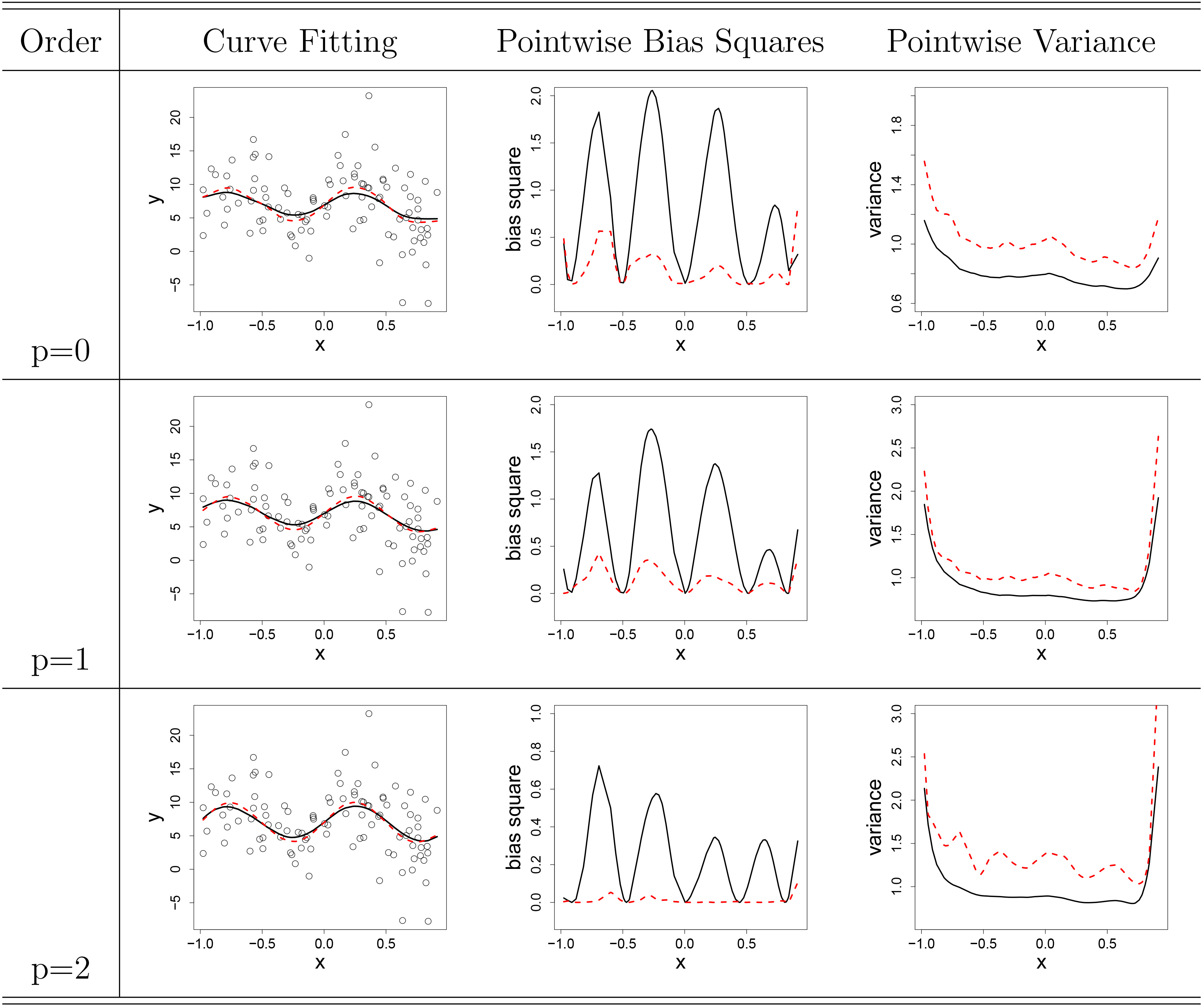$\epsilon\sim N(0,4)$ . Note: the dashed line is for DPI, and the solid line is for CV.

Second, for case (b) under $\epsilon\sim N(0,\sigma^{2})$ , we have that $\hat{h}_{0,CV}<\hat{h}_{\textit{DPI}}$ if $\sigma^{2}=$ 1, and $\hat{h}_{0,CV}>\hat{h}_{\textit{DPI}}$ if $\sigma^{2}=$ 4. This implies that the behaviour of pointwise squared bias and pointwise variance may be different under different $\sigma$ . From our simulation results, the squared bias of DPI is slightly larger than the CV method, and the difference of variance between two method is small. Surprisingly, as $\sigma^{2}=$ 4 in Fig. 2, the squared bias of the CV method is significantly larger than DPI, and the difference of variance is larger than the case of $\sigma^{2}=$ 1. In Table 2, MISE of $\hat{m}_{\textit{0,CV}}$ is less than MISE of $\hat{m}_{\textit{0,DPI}}$ ; for $\sigma^{2}=$ 4, on the other hand, MISE of $\hat{m}_{\textit{0,DPI}}$ is much smaller than MISE of $\hat{m}_{\textit{0,CV}}$ . In fact, from curve fitting in Fig. 2, we can see that curve $\hat{m}_{\textit{0,CV}}$ is flatter compared to $\hat{m}_{\textit{0,DPI}}$ . On the other hand, for $\epsilon\sim U(-\xi,\xi)$ , we can observe that the two bandwidths are close, especially as $\xi=$ 4. Hence, the curves for squared bias and variance are close and exhibit a similar pattern. For MISE, $\hat{m}_{\textit{0,CV}}$ is less than the MISE of $\hat{m}_{\textit{0,DPI}}$ as $\xi=$ 1, and $\hat{m}_{\textit{0,CV}}$ is slightly larger then MISE of $\hat{m}_{\textit{0,DPI}}$ . Compared to the case of $\epsilon\sim N(0,\sigma^{2})$ , we observe that the two methods do not have substantive difference when $\epsilon\sim U(-\xi,\xi)$ .

Figure 3.

Setting (c) with 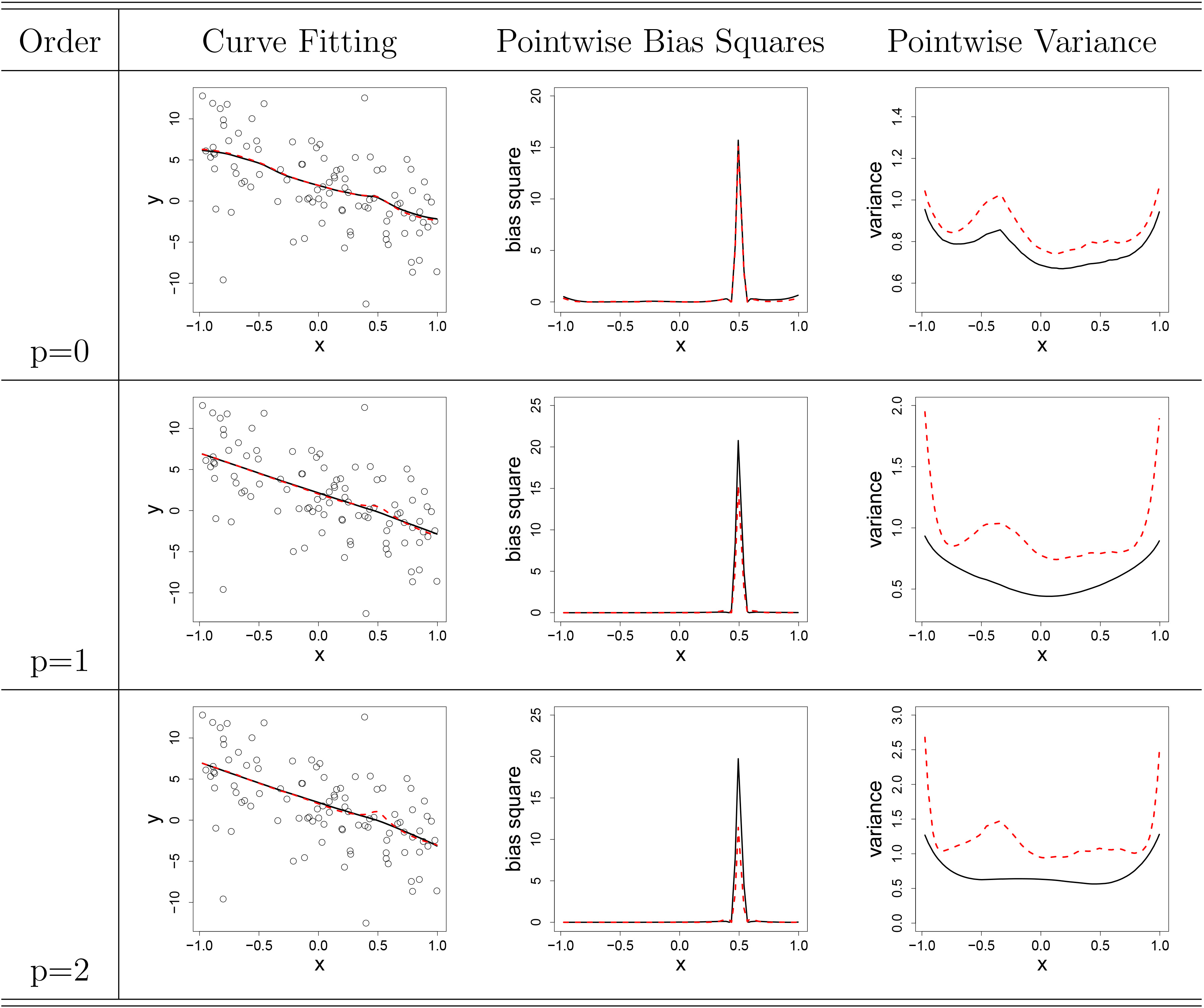$\epsilon\sim N(0,4)$ . Note: the dashed line is for DPI, and the solid line is for CV.

Lastly, for case (c) under $\epsilon\sim N(0,\sigma^{2})$ , we have that the bandwidth results are the same as in case (b). For $\sigma^{2}=$ 1, $\hat{h}_{\textit{DPI}}$ is even twice of $\hat{h}_{\textit{0,CV}}$ , so from our simulation results, it is expected that squared bias produced by DPI is much larger, and variance is relatively smaller. The situation is reversed when $\sigma^{2}=$ 4, as shown in Fig. 3. However, from the MISE criterion, values of $\hat{m}_{\textit{0,CV}}$ are both smaller. For $\epsilon\sim U(-\xi,\xi),\xi=$ 1, 4 based on our simulation results, we have $\hat{h}_{\textit{0,CV}}<\hat{h}_{\textit{DPI}}$ by a small margin. Hence, the squared bias and variance between both method are close, especially as $\xi=$ 4 in figures in our simulation results. From the MISE criterion, the values of $\hat{m}_{\textit{0,CV}}$ are smaller than values of $\hat{m}_{\textit{0,DPI}}$ .

3.1.2

p=

Next, we briefly interpret results for local linear estimation. As $p=$ 1, the CV bandwidths increase for all cases except $\epsilon\sim U(-1,1)$ , whereas DPI bandwidths are unchanged since they are always obtained by dpill(). Comparing CV and DPI methods, the direction of inequality start to change in some cases (e.g. case (c) under $\epsilon\sim U(-1,1)$ and $U(-4,4)$ ). In general, the analysis of squared bias and variance between the two methods is similar to the $p=$ 0 case. Interestingly, the MISE results start to differ from the $p=$ 0 case. In general, the DPI method outperforms the CV method. Besides those specific settings in our simulation studies, it is expected that the bandwidth obtained by dpill() perform better in local linear regression.

3.1.3 $p=$ 2

Finally, we briefly interpret results for local quadratic estimation. For $p=$ 2, it is interesting to see that the CV bandwidths are larger than that of DPI for all settings. It implies that pointwise squared bias and variance produced by the CV method are smaller and larger than the DPI method respectively. For MISE, the results under $p=$ 2 differ from $p=$ 1. Take case (b) as an example, as mentioned before, MISE of $\hat{m}_{\textit{1,DPI}}$ is smaller than MISE of $\hat{m}_{\textit{1,CV}}$ . Under $p=$ 2, however, MISE of $\hat{m}_{\textit{2,DPI}}$ is larger than MISE of $\hat{m}_{\textit{2,CV}}$ . On the other hand, some of the cases, like case (a), have the same results as $p=$ 1.

3.1.4 Remarks

Here we summarize and elaborate on the results above. First, for the overall comparisons under $p=$ 0, 1, 2, we see that values of (pointwise) squared bias and variance decrease as $p$ increase for both methods. For example, squared bias and variance under $p=$ 1 is obviously smaller than values in $p=$ 0. The theoretical justification outlined in Section 2.1 showed that bias under $p=$ 0 is larger than $p=$ 1. The numerical and graphical results obtained in the simulation validate these facts. As mentioned before, the value of pointwise variance depends on bandwidth. Hence, it is expected that variance under $p=$ 1 is smaller than $p=$ 0, since the bandwidth increases. Moreover, based on the analysis in Section 2.1, it is shown that MISE decreases as $p$ is large, which is also confirmed experimentally in Table 2.

Second, we briefly summarize the performances of two different bandwidth selection approaches. Though we reach a simulated-based conclusion, the cases and functional classes considered in Subsection 3.1 are sufficient to compare the bandwidth selection methods. From our simulations, we have a consistent observation.

In general, we see that the CV method performs better than the DPI method when $p=$ 0 and $p=$ 2, while DPI performs better when $p=$ 1. Hence, to get better estimators for both $p=$ 0 and $p=$ 2 in terms of minimizing MISE, the CV method will be the better choice; “dpill()” can still be applied for bandwidth selection for local linear estimators. Additionally, we argue that the “dpill()” function should not be casually used, when $p\neq 1$ , for the purpose of achieving precise estimator.

3.2 Estimating the level function of a binary response

Table 3
Bandwidth under three different situations for GLM

Case	$\hat{h}_{\textit{0,CV}}$	$\hat{h}_{\textit{1,CV}}$	$\hat{h}_{\textit{2,CV}}$	$\hat{h}_{\textit{DPI}}$
(a)	0.696	1.599	3.340	0.530
(b)	2.864	3.058	2.874	0.121
(c)	0.325	2.623	3.437	0.272

Figure 4.

GLM Under Setting (a), (b) and (c). Note: the dashed line is for DPI, and the solid line is for CV.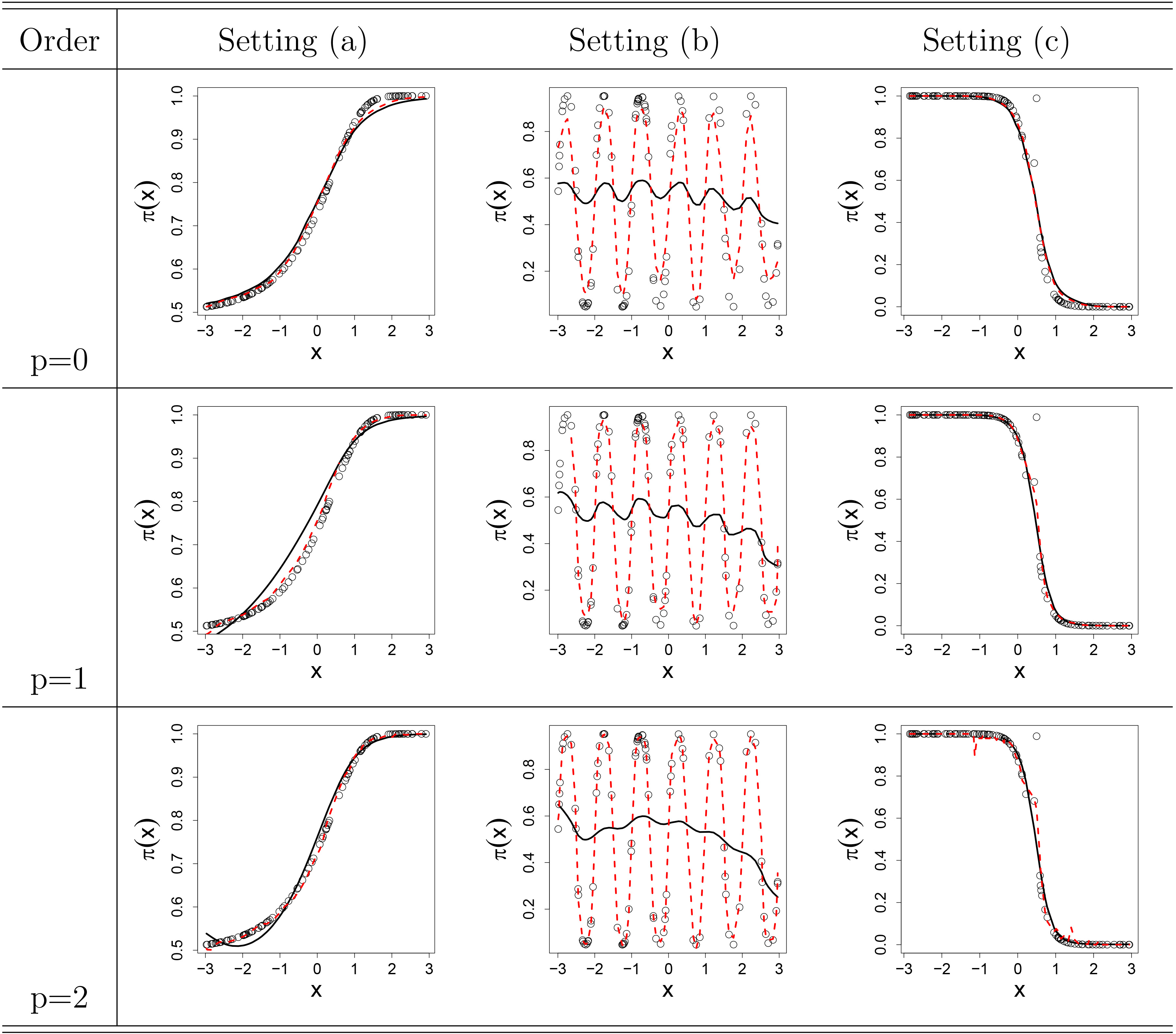

Consider the model of the form in Eq. (11). Following the idea from Section 3.1, we perform the simulation 1000 times for each of the following three underlying functions:

(a)

Monotone increasing function: $m(x)=\exp(x)$ ;

(b)

Periodic function: $m(x)=3\sin(2\pi x)$ ;

(c)

General function: $m(x)=2-5x+5\exp(-400(x-0.5)^{2})$ .

By the analysis we introduced in Section 2.2, we find bandwidth first and then obtain estimators $\hat{m}$ , or equivalently, $\hat{\pi}(x)$ . In each case, we calculate bandwidth in each simulation, so we have 1000 bandwidth values. We take the average among them and summarize them in Table 3. Surprisingly, in Table 3 the bandwidths obtained by the CV method are all larger than the bandwidths by the DPI method. In fact, it is interesting to observe that the CV score occasionally hit the upper bound. The intuitive reason is that log-likelihood of binary distribution is monotonic, and the CV score is constructed by minus log-likelihood. Hence, the CV score is monotonically decreasing instead of a quadratic form. After that, we find $\hat{\pi}(x)$ for the three different cases. Here we follow the same notations to represent bandwidth by CV and DPI respectively.

For case (a) in the first column of Fig. 4, we can see that CV and DPI are similar under $p=$ 0, but the curve for DPI is a better fit. For $p=$ 1, however, the fit for CV is not better than DPI, especially when $x\in[-2,1]$ . We see similar results for $p=$ 2, with the DPI curve fitting well. It is obvious, for case (b) in the second column in Fig. 4, that the curve for CV has a worse fit. Additionally, the curves are relatively flat and do not show any information about the true model. From the perspective of bandwidth, since the bandwidth for the CV method is significantly large, the curve generated by CV is much smoother, and would produce relatively large bias. Instead, the curve for DPI indeed shows the periodicity of the function. Finally, for case (c), we observe from the third column in Fig. 4 that performances between both methods are comparable under $p=$ 0, 1, 2.

From the graphical results, it is surprising that the DPI method performs better than the CV method in general, especially in case (b). We find that the CV method produces a larger bias and the curve fitting is worse than the DPI method. In addition, from case (a) and case (c), DPI method also fits better. Furthermore, it is interesting to note that DPI method always performs well for all orders $p$ and for all cases. This result is totally different from the result in the continuous response in Subsection 3.1.

3.3 Estimating the first order derivative of a continuous response

In some cases, we wish to estimate the derivative of a function. This is usually the case when the goal is the identification of local maxima and minima. Although this is not always the case, for our purposes we focus on the behavior of the derivative around zero. Specifically, we explore the estimation of the first derivative under quadratic kernel fit. The question is how the choice of bandwidth effects the identification of critical points (points such that $m^{\prime}(x)=$ 0). In Song et al. (2006), they explored this issue through 3 simulation studies. We mirror their analysis here in similar spirit but shifting our focus on the performance on a per bandwidth basis.

In the first simulation study, we examine the effects of cusp points. That is, points at which the function is continuous but the derivative does not exist. For example, the following function has a cusp and global maxima at $x=$ 2:

$\displaystyle m(x)=-2|x-2|.$ (18)

Cusps are of particular importance due to the behavior of the derivative. As we know, the derivative doesn’t exist at $x=$ 2, yet we want our estimate to still show that a local maximum is identified. That is, we require the derivative to equal zero somewhere in the neighborhood of the maximum. Referring to Table 4, we find that DPI provides a lower bandwidth estimate, as well as better coverage for the identified peak point. This is the ideal case since DPI does not over-smooth but still identifies the maximum.

Table 4

Mean bandwidth and coverage rate for derivative and $x_{0}$

$\sigma^{2}$	Case	$E(h)$	$\hat{\theta}(2)$	$x_{0}=$ 2
1	$\hat{h}_{\textit{CV}}$	0.914	0.927	0.701
	$\hat{h}_{\textit{DPI}}$	0.473	0.937	0.942
4	$\hat{h}_{\textit{CV}}$	1.378	0.932	0.872
	$\hat{h}_{\textit{DPI}}$	0.604	0.951	0.953

In the second simulation, we examine the empirical power of the test. This is particularly relevant because power is equivalent to $1-\beta$ where $\beta$ is the type II error. We want certainty in our identification, and thus are tolerant of type I error but sensitive to type II error. Hence, the more powerful test minimizes the type II error. Namely, we consider the following null hypothesis:

$\displaystyle m(x)=-3x^{2}+1,H_{0}:m^{\prime}(0)=0.$ (19)

In our earlier simulation, we found that DPI controlled type I error better, and referring to Fig. 5, we see that DPI is also a more powerful statistic. Again, this is an ideal case, since DPI does not over-smooth but is still more powerful than CV.

Figure 5.

Empirical power function.

In the final simulation, we examine the effect of multiple local maxima. We proceed in a similar vein to our cusp example, and enforce that one maxima be smooth and one be a cusp. Specifically, we use the example used in Song et al. (2006):

$\displaystyle m(x)=\left\{\begin{array}[]{ll}-2|x-1.5|,&\text{for }x<2.5,\\ -3(x-3.5)^{2}+1,&\text{o.w.}.\end{array}\right.$ (20)

Referring to Table 5, we see that DPI still outperforms CV in terms of coverage rates. Like the earlier examples, this is ideal because DPI does not over-smooth to outperform CV.

Table 5

Mean bandwidth and coverage rate for derivative and $x_{0}$ , $x_{1}$

$\sigma^{2}$	Case	$E(h)$	$\hat{\theta}(1.5)$	$x_{0}=$ 1.5	$\hat{\theta}(3.5)$	$x_{1}=$ 3.5
1	$\hat{h}_{\textit{CV}}$	0.551	0.751	0.968	0.750	0.810
	$\hat{h}_{\textit{DPI}}$	0.332	0.951	0.965	0.945	0.931
4	$\hat{h}_{CV}$	1.038	0.450	0.978	0.641	0.864
	$\hat{h}_{DPI}$	0.450	0.888	0.969	0.909	0.915

To conclude, we find that $\hat{h}_{\textit{DPI}}$ performs better in all three simulations. Namely, it provides better coverage rates for cusp and multiple maxima, compared to its CV counterpart. Further, in simulation 2 we find that hypothesis testing with DPI selected bandwidth provides more statistical power. We will reexamine this in our analysis of the yeast genome data.

4. Empirical study

In this section, we provide three empirical studies: one with a set of cyclical-pattern data, another is with the binary response and the last one is for the estimation of derivatives.

4.1 Weather data

We employ a set of cyclical-pattern data – daily temperature records and implement data analysis using the estimation and bandwidth selection methods introduced above. Essentially, the purpose of this analysis is to apply the first three orders of local polynomial kernel estimators with CV-/DPI-selected bandwidth to estimate the underlying temperature functions and compare the goodness of fit.

The Quality Controlled Local Climatological Data (QCLCD), from the National Climatic Data Center (NCDC), consists of hourly, daily, and monthly climatic information summaries for approximately 1,600 U.S. locations. Our sample contains the daily maximal temperature reports from 791 of the stations, covering from January 01, 2015 to December 31, 2015, which forms a panel of 365-time observations and 791 cross-sections.1

Ramsay (2006) applied a non-parametric recovery to the mean monthly temperatures for Canadian weather stations, assuming temperature records from different stations have the same underlying properties, which are primarily sinusoidal in character and certainly periodic over the annual cycle. For our data set, we simply assume, without further tests, that the temperature records from all stations follow the same underlying structure up to the sense that a curve-by-curve fitting by the local polynomial kernel estimators with the same order of polynomial and the same kernel can be implemented to all stations, while the estimation for different stations can have their own smoothing parameters, so that the six estimators ( $\hat{m}_{\textit{0,CV}}$ , $\hat{m}_{\textit{1,CV}}$ , $\hat{m}_{\textit{2,CV}}$ , $\hat{m}_{\textit{0,DPI}}$ , $\hat{m}_{\textit{1,DPI}}$ , $\hat{m}_{\textit{2,DPI}}$ ) are comparable.

Our estimation results, consistent with the simulation results, show that $\hat{h}_{\textit{DPI}}$ ’s, in general, lead to much smoother estimated curves than any of CV-selected bandwidths do, while the performance of the estimators with CV-selected bandwidths is relatively similar. From another point of view, according to our numerical results, which presents the average level of each bandwidth as well as the sum of squared error (SSE) for each estimator, the three average levels of the CV-selected bandwidth are relatively close and much smaller than the DPI-selected bandwidth. It also verifies the simulated-based conclusion in Subsection 3.1.4. The corresponding figures and the numerical results can be requested from the author.

4.2 Graduate school admission rates

As an example of the binary response case, we employ a set of data, including the GRE (Graduate Record Exam) scores, GPA (grade point average) and admission into graduate school for 400 individuals.2 The response variable, admit/not admit, is a binary variable; the GRE scores and the GPA are treated as continuous.

In essence, the results are consistent with the simulation results in that the DPI-selected bandwidth is smaller than then the CV-selected bandwidth, and thus the CV-generated estimated curves are smoother than the DPI-generated curves. For the estimation result itself, it shows that in general, higher GRE and GPA score will help to increase the probabilities of getting admitted up to around 50%. The corresponding figures and the numerical results can be requested from the author.

4.3 Yeast genome dataset

In this section, we analyze a subset of the oligonucleotide microarray of yeast. This dataset was used by Song et al. (2006) to demonstrate the strength of their nonparametric kernel smoothing technique. The purpose of our analysis now is to see the effects of bandwidth selection procedures on the estimation of local maxima, or peaks, in hybridization intensity profiles. We are concerned with peaks because they correspond to autonomous replication sequences, containing the putative origin of replication, which is of importance to genetics.

To help contrast the bandwidth selection procedures, we adopt the same methodology by Song et al. (2006) and estimate the first derivative of the hybridization intensity profile curve with quadratic kernel smoothing. Our main question is whether CV selected bandwidth is better than direct plug-in methods. By computations, the bandwidth values determined by the CV and DPI methods are 0.684 and 1.444, respectively. Analysis by Song et al. (2006) relied on the built-in R function “dpill()” for DPI bandwidth estimates, but again, this approach is questionable since “dpill()” is known for local linear kernel estimation. Therefore, we would expect that bandwidth selected by “dpill()” is not optimal.

In our analysis, however, we find that the purported suboptimal bandwidth selection by “dpill()” does not present a problem in the identification of peaks. Bandwidth acts as a smoothing parameter in a kernel regression setting and “dpill()” tends to overestimate the bandwidth compared to CV. This can easily be seen from the peak estimates in our numerical results, where the peaks identified by CV form a superset of the peaks identified by DPI. The corresponding numerical tables can be requested from the author.

First of all, we identify the peaks using the estimates of the first derivative. There are two cases of equilibrium points that we analyze. For Case I, we look for a positive first derivative estimate followed by a negative one. By the mean value theorem, we know that a continuous function will possess extrema somewhere in that interval, and we take the point estimate closest to zero. The Case II equilibrium point is unique and is found by considering all confidence intervals that contain zero and taking the corresponding point estimate that is closest to zero. The corresponding results of figures can be requested from the author.

Second, we obtain confidence intervals for chromosomal coordinates by a local inversion technique. That is, we know that the inverse of the lower 95% confidence interval for the derivative provides the maximum of the 95% confidence interval for the chromosomal coordinate, as well as vice-versa. Then we do a search for the point estimate that is closest to the lower/upper confidence interval and takes the value that minimizes the absolute difference. Since we are using a Gaussian kernel, this confidence interval is symmetric and so we mirror the half confidence interval. In our comparisons, we also provide the point estimate and confidence interval for each peak, where the corresponding results of figures can be requested from the author.

In summary, we find that identification issues typically arise only if the bandwidth is too low, which results in the degenerate estimation of peaks (e.g. overlapping peaks/confidence intervals and overabundance near the end-points of the data). Some of these problems, such as the problem at endpoints, can be fixed by simply ignoring them as spurious estimates. However, multiple identified peaks in a small region present a persistent problem in deciding which (if any or perhaps all) are true peaks.

5. Discussion

In this article, we illustrate the comparison between the CV method and the DPI method through the simulation study, considering both the continuous response case and the binary response case. From the comprehensive simulations, we conclude that the DPI method performs better than the CV method when $p=$ 1 under the MISE criterion. However, the CV method performs better than DPI when $p=$ 0, 2. It also tells us that we cannot casually use “dpill()” to obtain the bandwidth if we want to fit either local constant or local quadratic estimator. On the other hand, we recommend using “dpill()” when we fit the local linear estimator. Different from the continuous response, DPI method always performs well in the binary response. Hence, we may conclude that “dpill()” is welcomed to use when fitting the binary response.

However, since the function “dpill()” is predetermined based on linear estimators, one possible extension of our study would be to generalize DPI to all $p\in\mathbb{N}$ , so that we can discuss the performance of CV and DPI more precisely for $p\neq 1$ . Second, in Section 2.2, we use a binary response as our GLM example. In fact, we can also consider other types of data (e.g., count data in Poisson regression). Moreover, theoretical results can be derived to show a more rigorous comparison between the two bandwidth selection methods.

Although we mainly study bandwidth selection for $p=$ 0, 1, 2 based on model Eq. (1), we can even investigate $p=$ 3 or even higher order. Besides, there are also many extensions which we can explore. For example, we can examine the comparisons with $\textit{AIC}_{c}$ bandwidth selection proposed by Hurvich et al. (2002). In addition, studying the comparisons of bandwidth selection for the extensive models, such as single index model, generalized additive model (GAM) or even non-parametric model with high-dimensional covariates, is also an important problem. Finally, Hall and Racine (2015) discussed CV over both the bandwidth and the order of the polynomial using the R package crs. It would be interesting to examine the use of the crs package in context of the methods discussed in this paper. A future research project is planned to investigating such an application of the crs package.

Footnotes

The 791 stations are chosen by eliminating the stations with missing data during 2015, and no other sampling scheme is employed.

The data can be obtained from http://www.ats.ucla.edu/stat/stata/dae/binary.dta.

Acknowledgments

The author would like to extend the great gratitude to an Editor, an Associate Editor and a reviewer for valuable suggestions and useful comments to make this paper be better. The author also extends his great gratitude to Dr. Pengfei Li, an associated professor in the Department of Statistics and Actuarial Science, University of Waterloo, for his generous help, valuable advice and guidance on this project.

References

Bowman,

A. W.

(1984). An alternative method of cross-validation for the smoothing of density estimates, Biometrika, 71, 353-360.

Cleveland,

W. S.

, & Loader,

(1996). Smoothing by local regression: Principles and methods. Statistical Theory and Computational Aspects of Smoothing, Springer, p. 10-49.

Fan,

, & Gijbels,

(1992). Variable bandwidth and local linear regression smoothers. The Annals of Statistics, 20, 2008-2036.

Fan,

, & Gijbels,

(1995). Data-driven bandwidth selection in local polynomial fitting: variable bandwidth and spatial adaptation. Journal of the Royal Statistical Society. Series B, 57, 371-394.

Fan,

, & Gijbels,

(1996). Local Polynomial Modelling and Its Applications. CRC Press.

Hall,

P. G.

, & Racine,

(2015). Infinite order cross-validated local polynomial regression. Journal of Econometrics, 185, 510-525.

Hurvich,

C. M.

Simonoff,

J. S.

, & Tsai,

C.-T.

(2002). Smoothing parameter selection in nonparametric regression using an improved Akaike information criterion. Journal of the Royal Statistical Society. Series B, 60, 271-293.

Li,

, & Racine,

J. S.

(2007). Nonparametric Econometrics: Theory and Practice. Princeton University Press.

Loader,

(1996). Change point estimation using nonparametric regression. The Annals of Statistics, 24, 1667-1678.

10.

Loader,

C. R.

(1999). Bandwidth selection: classical or plug-in? The Annals of Statistics, 27, 415-438.

11.

Newell,

, & Einbeck,

(2007). A comparative study of nonparametric derivative estimators. in Proc. of the 22nd International Workshop on Statistical Modelling.

12.

Ramsay,

J. O.

(2006). Functional Data Analysis, Wiley.

13.

Rudemo,

(1982). Empirical choice of histograms and kernel density estimators. Scandinavian Journal of Statistics, 9, 65-78.

14.

Ruppert,

Sheather,

S. J.

, & Wand,

M. P.

(1995). An effective bandwidth selector for local least squares regression. Journal of the American Statistical Association, 90, 1257-1270.

15.

Song,

P. X.-K.

Gao,

Liu,

, & Le,

(2006). Nonparametric inference for local extrema with application to oligonucleotide microarray data in the yeast genome. Biometrics, 62, 545-554.

16.

Stone,

C. J.

(1977). Consistent nonparametric regression. The Annals of Statistics, 5, 595-620.

17.

Wand,

M. P.

, & Jones,

M. C.

(1994). Kernel Smoothing. CRC Press.

18.

Woolhouse,

(1870). Explanation of a new method of adjusting mortality tables; with some observations upon Mr, Makeham’s modification of Gompertz’s theory. Journal of the Institute of Actuaries and Assurance Magazine, 15, 389-410.

19.

Xia,

, & Li,

(2002). Asymptotic behavior of bandwidth selected by the cross–validation method for local polynomial fitting. Journal of Multivariate Analysis, 83, 265-287.

20.

Zambom,

A. Z.

, & Dias,

(2012). A review of kernel density estimation with applications to econometrics. arXiv preprint arXiv:1212.2812.

Investigating effects of bandwidth selection in local polynomial regression model with applications

Abstract

Keywords

1. Introduction

2. Estimation procedure

2.1 Continuous response

3.1 Estimating the level function of a continuous response

3.1.3 p = 2

3.1.4 Remarks

3.2 Estimating the level function of a binary response

Table 3 Bandwidth under three different situations for GLM

4.1 Weather data

4.2 Graduate school admission rates

4.3 Yeast genome dataset

5. Discussion

Footnotes

Acknowledgments

References

3.1.3 $p=$ 2

Table 3
Bandwidth under three different situations for GLM