Probability space of regression models and its applications to financial time series

Abstract

We introduce a notion of a probability space of regression models and discuss its applications to financial time series. The probability space of regression models $\mathcal{L}=(\mathcal{M},\wp)$ consists of a set of regression models $\mathcal{M}$ and a probability measure $\wp$ , which is based on the model “quality”, i.e. its ability to “fit” into historical data and to forecast the future values of the target variable. The set of regression models $\mathcal{M}$ is assembled by selecting various combinations of input variables with different lags, transformations, etc., and varying historical data sets that are used for model building and validation. It is assumed that the model set $\mathcal{M}$ is “complete” in the sense that it exhausts all the “meaningful” regression models that are possible to be built given available historical data and independent variables. Each model $M$ from the set $\mathcal{M}$ yields a scenario $y(t;m)$ for the target variable $y$ , and thus the probability space of regression models $\mathcal{L}=(\mathcal{M},\wp)$ allows one to build a probability distribution for $Y(t)$ for each projection time $t$ . We demonstrate how those distributions can be used to estimate risk capital reserves required by the regulators for large U.S. banks for credit and operational risks under the macroeconomic scenarios provided by the Federal Reserve Bank (FRB) for the Comprehensive Capital Analysis and Review (CCAR) stress testing.

Keywords

Regression models probability space financial time series capital stress testing

“The recognition of risk management as a practical art rests on a simple clich? with the most profound consequences: when our world was created, nobody remembered to include certainty. We are never certain; we are always ignorant to some degree. Much of the information we have is either incorrect or incomplete.”

– Peter L. Bernstein

1. Introduction

The challenge of dealing with a financial time series can be formulated in its most general form as the following: given all the information available at the moment (data, results of analysis, expert opinions, etc.), find out what should be expected from this financial time series in the future. Common examples would include assessing future time development of credit losses, operational risk losses, mortgage default and prepayment, likelihood of a corporate bond default, etc., given available historical data on time development of such possible explanatory (independent) variables as industry and macroeconomic factors, interest rates, unemployment index, borrowers’ characteristics, etc. From the perspective of risk management, an ideal solution would be finding probability distributions of possible financial time series values for the projection times of interest.

In more formal settings. Let $K(t_{0})$ be a complete body of knowledge (data, results of analysis, expert opinions, etc.) available about a financial time series $y(t)$ at the time $t_{0}$ . Find probability distributions

$\displaystyle\{Y(t_{1})|K(t_{0}),P(t_{1})|K(t_{0})\},\{Y(t_{2})|K(t_{0}),P(t_{% 2})|K(t_{0})\},\dots,\{Y(t_{J})|K(t_{0}),P(t_{J})|K(t_{0})\}$ (1)

of the financial time series $y$ for the projection times $t_{0}<t_{1}<t_{2}<\dots<t_{J}$ .

The notation used in the Eq. (1) explicitly reflects the fact that both elements of the pair $\{Y(t_{j}),P(t_{j})\}$ , possible values $Y(t_{j})$ that the time series $y(t)$ can take at $t_{j}$ and their corresponding probabilities $P(t_{j}),$ are conditional upon the knowledge $K(t_{0})$ that is acquired at $t_{0}$ .

In this paper we introduce the notion of Probability Space of Regression Models (PSRM) as a comprehensive attempt to build a probability distribution $\{Y(t)|K(t_{0}),P(t)|K(t_{0})\}$ for $t>t_{0}$ . The fundamental assumption underlying PSRM is that the body of knowledge $K(t_{0})$ consists of “meaningful” regression models that can be built for time series $y(t)$ using available historical data. The objective for creating a PSRM is NOT necessarily to build the best model – the chance of developing a crystal ball is rather slim – we want to learn about ALL possible outcomes “suggested” by ALL meaningful regression models.

The choice of regression as the only modeling framework is driven to a certain degree by the necessity to be able to explain the modeling results to various regulation and consumer protection authorities which are very reluctant to accept any model (e.g., neural network) that lacks clear explanations of how the model inputs impact its output. It was observed (see, for example, Hastie et al., 2001) that “For prediction purposes they [linear regression models] can sometimes outperform fancier nonlinear models, especially in situations with small numbers of training cases, low signal-to-noise ratio or sparse data.”

The key reason for creating and employing a PSRM is developing a probability framework that encompasses and formalizes the model building process which is commonly employed in risk management. The process starts with the project’s business objectives and continues with selecting the data, choosing predictors, evaluating and using the models. All those steps whilst driven mostly by the project objectives and data availability have unavoidably some subjectivity. The employment of a PSRM allows one to make this subjectivity to be clearly stated and recognized. When all decisions are made and all meaningful models are built, the PSRM allows one to see a clear probabilistic picture of what should be expected from the financial times series of interest during the projection period.

The paper adheres to the following outline: Section 2 introduces the notion of Probability Space of Regression Models (PSRM) and provides a simple example illustrating in detail how a PSRM can be built and used for risk assessment and hedging of a financial time series. Section 3 discusses the general approach to creating PSRMs – building sets of regression models and defining corresponding model probabilities. Section 4 describes how PSRMs can be used to estimate risk capital reserves required by the regulators for large U.S. banks for credit and operational risks under the macroeconomic scenarios provided by the Federal Reserve Bank (FRB) for the CCAR stress testing. Finally, in Section 5 we present some of our conclusions.

2. An example of probability space of regression models (PSRM)

Let $y(t)$ be a financial time series of interest (i.e., credit losses, operational risk losses, mortgage default and prepayment, likelihood of a corporate bond default, etc.). By $\mathcal{M}(t_{0})=\{M_{j}(t_{0}),∼{}j=1,\dots,J\}$ we denote a set of all meaningful regression models that could be built using available historical data for both the target $y(t)$ and the predictors as of time $t_{0}$ . Let us assume that for each model $∼{}M_{j}(t_{0})\in\mathcal{M}(t_{0})$ one defines a numeric value $P_{j}(t_{0})$ $\in[0,1]$ which is proportional to the “quality” of the model $M_{j}(t_{0}),∼{}$ i.e. model’s ability to “fit” into historical data and to forecast the future values of the target variable. The pair

$\displaystyle\mathcal{L}(t_{0})=(\mathcal{M}(t_{0}),\wp(t_{0})),\wp=\{P_{j}(t_% {0}),∼{}j=1,\dots,J\}$

is defined as Probability Space of Regression Models (PSRM). Note that since the set $\mathcal{M}(t_{0})$ encompasses all meaningful regression models, it is assumed to be complete, i.e.

$\displaystyle\sum^{J}_{j=1}{P_{j}(t_{0})}=1.$

Note that for this case, the complete body of knowledge $K(t_{0})$ consists of the historical data available at the time $t_{0}$ for both predictors and the target, the set of meaningful models $\mathcal{M}(t_{0})=\{M_{j}(t_{0}),∼{}j=1,\dots,J\}$ , and the corresponding probabilities $\wp(t_{0})=\{P_{j}(t_{0}),∼{}j=1,\dots,J\}.$ From here on, we will be omitting the time $t_{0}$ in the notations assuming that PSRM $\mathcal{L}=(\mathcal{M},\wp)$ is built as of the latest $t_{0}$ for which the data are available.

The word “meaningful” is a key word in building a set of regression models $\mathcal{M}$ for a PSRM. The meaningfulness of a model is defined by a set of criteria which combines requirements to model quality with business matter expert opinions about how a particular independent variable should affect the target variables. The latter usually takes the form of requirements to the signs of regression coefficients. For example, it is well known that the frequency and severity of credit losses for consumer loans are positively correlated with unemployment and negatively correlated with the GDP growth rate. Thus, for a model built to assess time development of consumer loss frequency/severity, the coefficient for the unemployment variable is expected to be positive and the one for the GDP growth to be negative. The former usually has two types of requirements: one assessing how well a model fits into the historical data that was used for model building and the other evaluating the model accuracy in predicting out-of-time values. For example, it can be decided that only the models with $R^{2}>25\%$ , all $p$ -values of the coefficient $t$ -statistics below 20%, and the root-mean-square error (RMSE) for the out-of-time period less than 15% are included into the set of regression models $\mathcal{M}$ . Obviously, in some real life situations, there might be NO meaningful regression models.

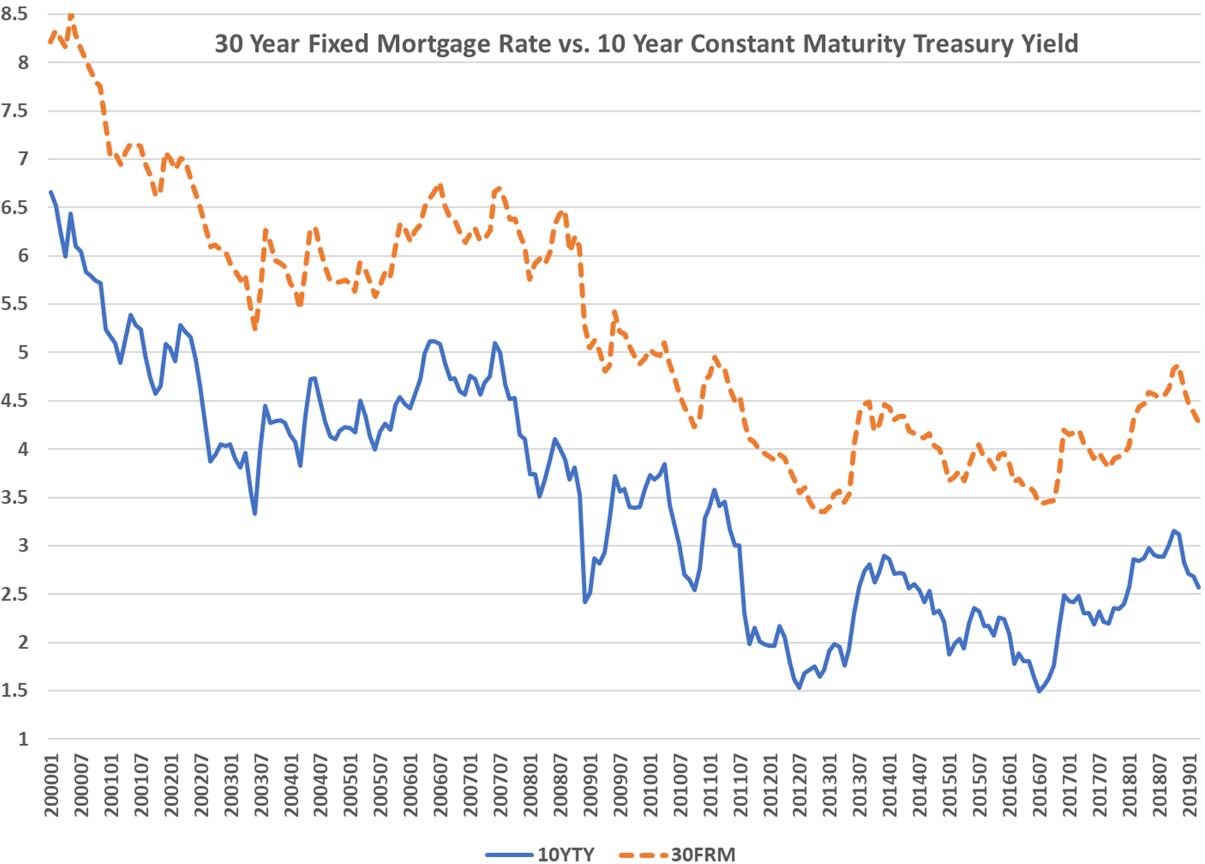
Let us consider a simple example of building and applying a PSRM for risk management and hedging. In this example, the financial time series of interest is the 30-year Fixed Mortgage Rate (30FRM). This rate is heavily used by the mortgage industry to price and hedge fixed-rate 30-year mortgages (see, for example, (Young, 1997)), and it is traditionally assessed through the spread between 30FRM and 10-year Constant Maturity Treasury Yield (10YTY). So for this example, the target variable $y(t)$ is the difference between 30FRM and 10YTY reported monthly. To better illustrate how a PSRM can be created and used, we limit the model inputs to just variable 10YTY and build regression models that takes 12 monthly projections for 10YTY and yields 12 monthly projections for the 30FRM-10YTY Spread.

The historical data that were used in model building and testing (please see Fig. 1) cover the period of January 2000 through March 2019 (please see (Economic Research Division, March 2019) for 10YTY and ((FedPrimeRate, March 2019) for 30FRM). The last 12 months of this period were used to replicate the real life situation: given 12 monthly projections of 10YTY, assess ALL possible 30FRM – 10YTY spread outcomes “suggested” by ALL meaningful regression models.

Figure 1.

30-year Fixed Mortgage Rate (30FRM) vs. 10-year Constant Maturity Treasury Yield (10YTY).

Figure 2.

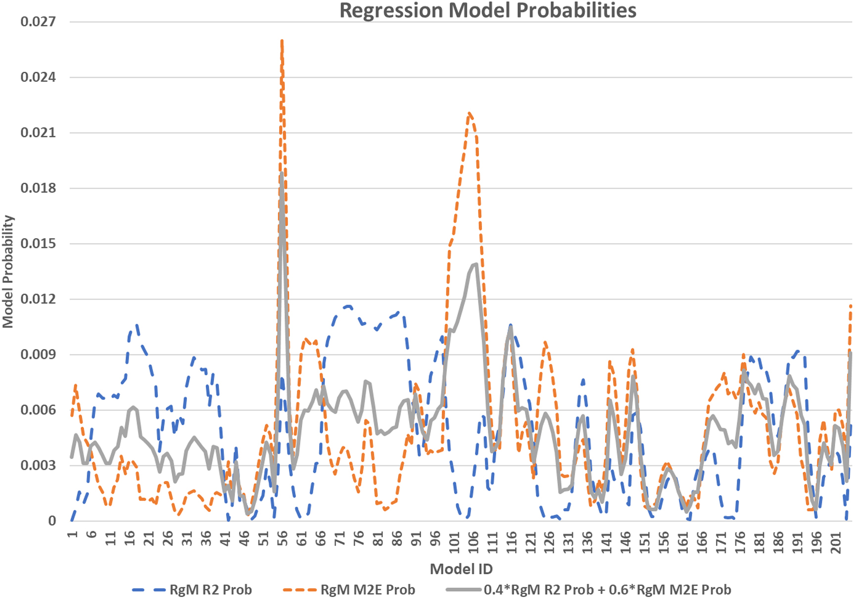
Historical fit $P_{R2}[M_{j}]$ , out-of-time accuracy $P_{\textit{RMSE}}[M_{j}],$ and combined $P_{\lambda=0.4,\mu=0.6}[M_{j}]$ for $M_{j}\in\mathcal{M}$ .

We say that a regression model $M:y=b_{0}+b_{1}x$ is meaningful if the following conditions are met:

$\displaystyle R^{2}[M]>0.4$ (2a) $\displaystyle pVt[M]\equiv\max_{j=0,1}\{pVt(b_{j})\}\leqslant 0.1$ (2b) $\displaystyle\textit{RMSE}[M]\leqslant 0.1$ (2c) $\displaystyle b_{1}<0$ (2d)

Here $pVt(b_{j})$ denotes the $p$ -value of the t-statistics for the model coefficient $b_{j}$ and $\textit{RMSE}[M]$ stands for the root-mean-square error (RMSE) for the out-of-time period. The coefficient $b_{1}$ for 10YTY is required to be negative since a higher 10YTY usually goes along with a smaller 30FRM – 10YTY spread.

The set $\mathcal{M}$ of total of 205 meaningful regression models satisfying Eqs (2a)–(2d) were built. For each model $M_{j}\in\mathcal{M}$ , a 12-month historical period was used to find the coefficients and the following 3 months were used to assess the accuracy in predicting out-of-time values. For example, for a model $M$ , the coefficients $b_{0}$ and $b_{1}$ along with $R^{2}[M]$ and $pVt[M]$ were calculated using the data for the period March 2014 through February 2015 and $\textit{RMSE}[M]$ was assessed using data for the period March 2015 through May 2015.

For each model $M_{j}\in\mathcal{M}$ , we define

$\displaystyle P_{R2}[M_{j}]=\frac{R^{2}[M_{j}]}{\sum_{M_{j}\in\mathcal{M}}{R^{% 2}[M_{j}]}}$ (3a) and $\displaystyle P_{\textit{RMSE}}[M_{j}]=\frac{\textit{RMSE}[M_{j}]}{\sum_{M_{j}% \in\mathcal{M}}{\textit{RMSE}[M_{j}]}}$ (3b)

$P_{R2}[M_{j}]$ can be interpreted as a numerical measure of the model $M_{j}$ ability to “fit” into historical data and $P_{\textit{RMSE}}[M_{j}]$ measures the model accuracy over the out-of-time period. Figure 2 above shows $P_{R2}[M_{j}]$ and $P_{\textit{RMSE}}[M_{j}]$ for all $M_{j}\in\mathcal{M}$ . As one can see, a high or low $P_{R2}[M_{j}]$ does not always come with a high or low $P_{\textit{RMSE}}[M_{j}]$ and vice versa.

Combining $P_{R2}[M_{j}]$ and $P_{\textit{RMSE}}[M_{j}]$ allows us to define the probability of $M_{j}\in\mathcal{M}$ by the following formula:

$\displaystyle P_{\lambda,\mu}[M_{j}]=\lambda\cdot P_{R2}[M_{j}]+∼{}\mu\cdot P_% {\textit{RMSE}}[M_{j}]$ (4)

for given $\lambda,∼{}\mu\in[0,1],∼{}∼{}\lambda+\mu=1$ . Equations (3) and (4) obviously imply that the value $P_{\lambda,\mu}[M_{j}]$ is proportional to model quality and $\sum_{M_{j}\in\mathcal{M}}{P_{\lambda,\mu}[M_{j}]=1}$ .

In general, the values of $\lambda$ and $\mu$ are decided upon by the perceived importance of good in-historical data fitting versus importance of good out-of-time-fitting. For this example, we have selected $\lambda=0.4$ and $\mu=0.6$ and considered PSRM

$\displaystyle\mathcal{L}=(\mathcal{M},\wp)\text{∼{}with∼{}}\wp=\{P_{j}=P[M_{j}% ]=0.4\cdot P_{R2}[M_{j}]+0.6\cdot P_{\textit{RMSE}}[M_{j}]\}$

We used the 12-month period $T=\{201804,\dots,201903\}$ of available historical data as a projection period, and for each month $t\in T$ the model $M_{j}\in\mathcal{M}$ yielded 30FRM – 10YTY spread forecast $y_{j}(t)$ . Thus, for each $t\in T$ we built an EDF

$\displaystyle Y_{\mathcal{L}}(t)=(Y(t),\wp),$

where $Y(t)=\{y_{j}(t),∼{}j=1,\dots,205\}$ is a set of projections yielded by $M_{j}$ for $t\in T$ .

It is important to note that while the values $y_{j}(t)$ might be different for different $t\in T$ , the corresponding probability $P_{j}=P[M_{j}]\in\wp$ stays the same for all $t\in T.$

For each $t\in T$ the EDF $Y_{\mathcal{L}}(t)=(Y(t),\wp)$ was fitted into a continuous distribution $F_{\mathcal{L}}(t)$ , which, in its turn, allows one to learn about ALL possible 30FRM – 10YTY spread values “suggested” by regression models $\mathcal{M}$ . Table 1 below shows the parameters and errors of fitted distributions.

Table 1

Parameters and errors of fitted distribution

Y(t) distribution fits with R2 weight $=$ 0.4 and RMSE weight $=$ 0.6
PrjYYYYMM	Gauss $\mu$	Gauss fit $\sigma$	Gauss fit err	Gamma fit $\alpha$	Gamma fit $\beta$	Gamma fit err
201804	1.895	0.507	0.0623	13.192	0.138	0.057
201805	1.863	0.504	0.0612	12.899	0.139	0.055
201806	1.883	0.506	0.0621	13.041	0.139	0.056
201807	1.889	0.506	0.0622	13.140	0.138	0.056
201808	1.889	0.506	0.0622	13.140	0.138	0.056
201809	1.857	0.503	0.0606	12.873	0.139	0.055
201810	1.819	0.498	0.0571	12.531	0.140	0.051
201811	1.827	0.498	0.0578	12.632	0.139	0.051
201812	1.906	0.510	0.0632	13.204	0.139	0.058
201901	1.943	0.516	0.0646	13.370	0.140	0.059
201902	1.952	0.517	0.0646	13.435	0.140	0.059
201903	1.984	0.523	0.0638	13.532	0.141	0.059

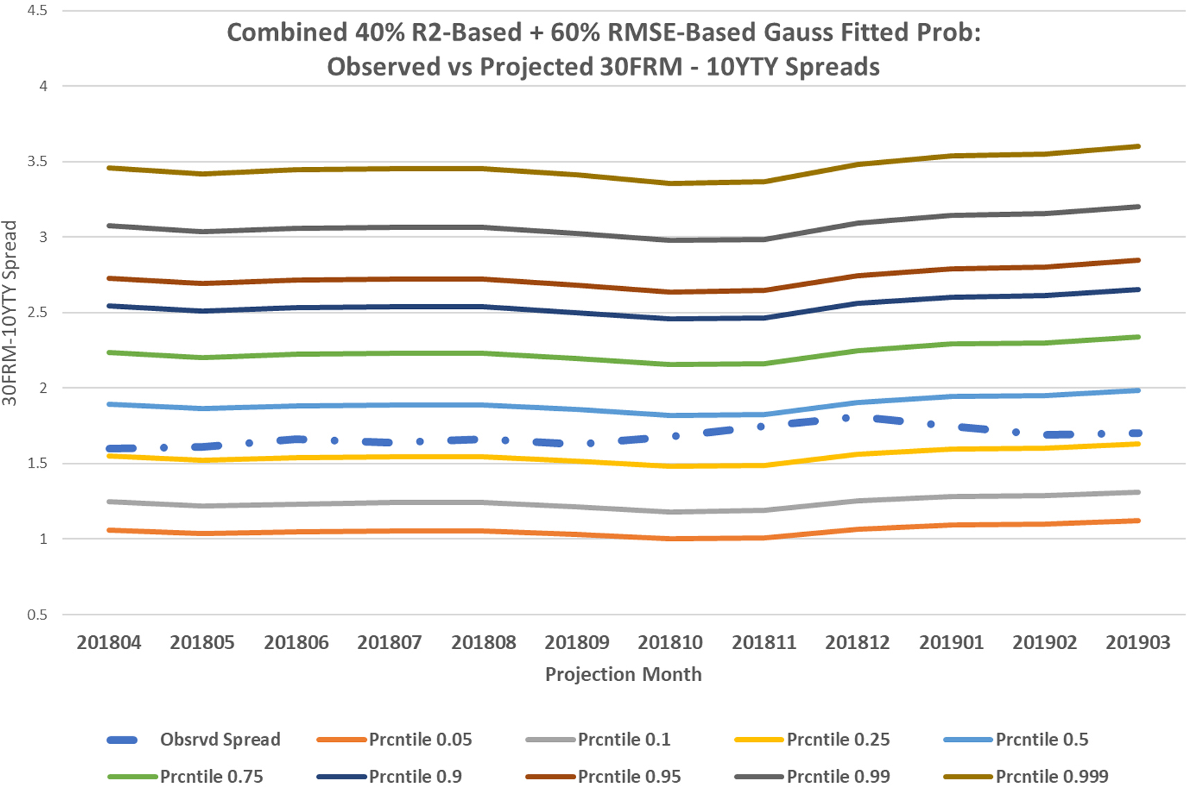
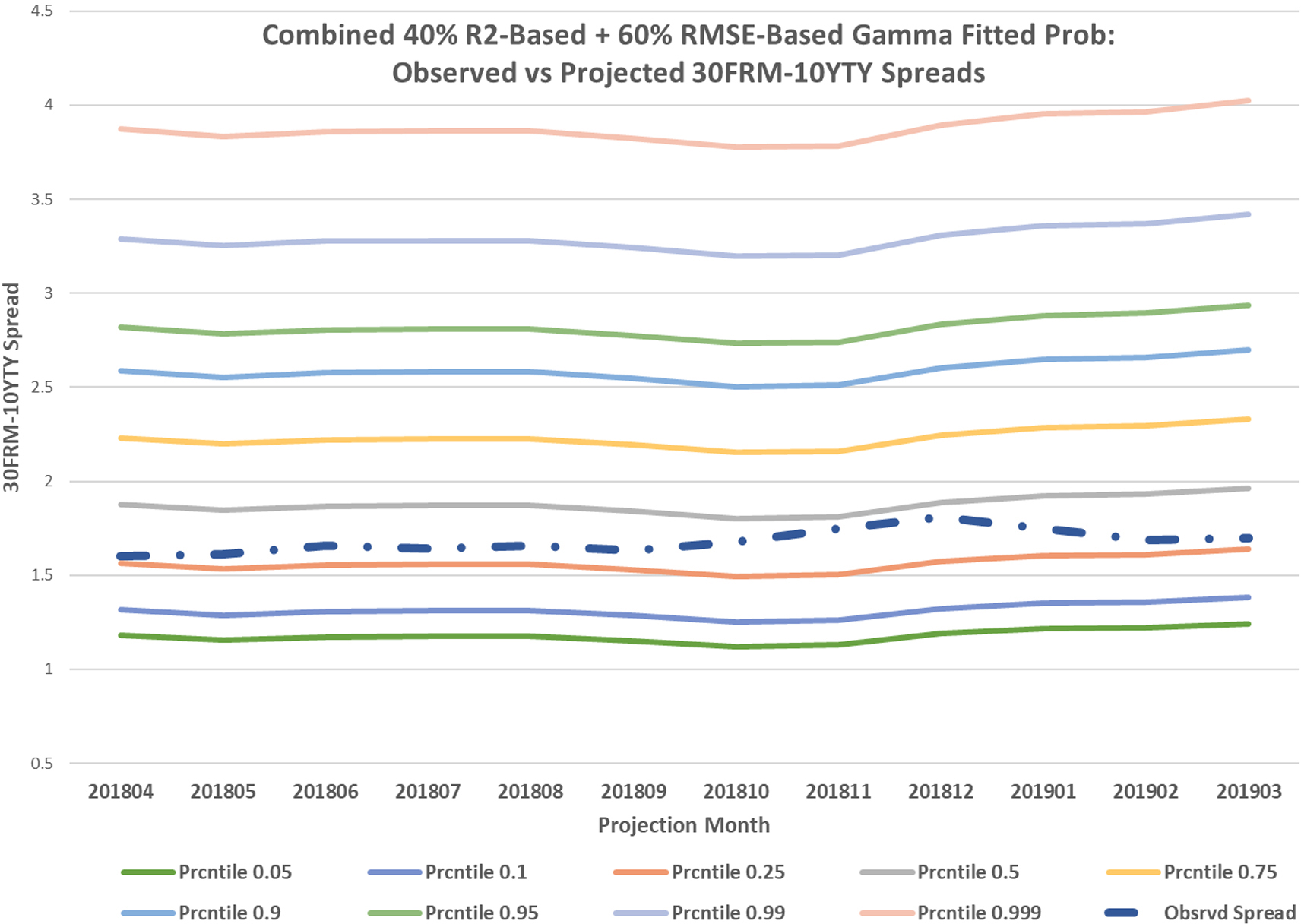
Figures 3 and 4 on the next page show various percentile levels of the 30FRM-10YTY Spread suggested by the PRSM for the projection months. The risk managers with portfolios exposed to the 30-year fixed rate mortgages could use those estimates to hedge their positions or allocate capital that is sufficient to cover potential losses.

Figure 3.

Percentile levels of the 30FRM-10YTY Spread for suggested by the PRSM with Gaussian fit for the projection months.

Figure 4.

Percentile levels of the 30FRM-10YTY spread for suggested by the PRSM with gamma fit for the projection months.

3. General approach to PSRMs

In the most general case, the objective for building a set $\mathcal{M}$ of regression models for a target variable $y(t)$ is to demonstrate that the available data and the independent variables under consideration can be used to build meaningful regression models for estimating time development of the target variable. As was mentioned earlier, the building efforts can result in proving that there are no meaningful regression models connecting the target variable to possible predictors.

In business settings the model set $\mathcal{M}$ is created by varying the following model specifications:

MS1: The independent variables that are used in a model. It is well-known that each independent variable requires a certain number of data records. So if one has a large number of variables “supported” by relatively few records, the number of variables used in a model should be restricted accordingly.

MS2: Lags for the independent variables that are used in a model. In many cases, the target is effected by the inputs with delays that vary from an input to an input.

MS3: Historical period that was used to build a model. This is undoubtedly the most important model specification. When a model is built using the data from a certain historical period, then the forecast yielded by this model is what can happen if the model projection period is “similar” to the historical data upon which the model was built.

MS4: Historical period that was used for out-of-time assessment of the model performance.

Formally, a regression model $M$ is described as a collection

$\displaystyle M=(Y,\vec{F},\vec{L},\vec{H},\vec{C},\vec{S}),$ (5)

where $Y$ is the target variable;

$\vec{F}=(F_{1},\dots,∼{}F_{J})$ are variable “participation” flags:

$\displaystyle F_{j}=\begin{cases}0,&\text{if variable $V_{j}$ is not used in % the model};\\ 1,&\text{if variable $V_{j}$ is used in the model}.\end{cases}$

$\vec{L}=(L_{1},\dots,L_{J})$ are variable lags:

$\displaystyle L_{j}=\begin{cases}-1,&\text{if variable $V_{j}$ is not used in % the model};\\ l\in\{0,1,\dots,l_{\max}\},&\text{if variable $V_{j}$ that is used in the % model}.\end{cases}$

$\vec{H}=(H_{1},H_{2},H_{3})$ are data history settings:

$H_{1}$ and $H_{2}$ are correspondingly the beginning and the length of the historical period that was used for model building, $H_{3}$ is the length of history that was used to assess the model performance over the out-of-time period.

$\vec{C}=(C_{1},\dots,C_{J})$ are model coefficients:

$C_{j}=\begin{cases}0,&\text{if variable $V_{j}$ is not used in the model};\\ \text{is defined by the model building procedure},&\text{if variable $V_{j}$ % is used in the model}.\end{cases}$

$\vec{S}=(S_{1},\dots,S_{N})$ is a set of statistics that are used to evaluate the model performance.

The set of meaningful regression models $\mathcal{M}$ is built by varying the vectors $\vec{F},\vec{L}$ , and $\vec{H}$ (please see MS1 through MS4 above) and by using the vectors $\vec{C}$ and $\vec{S}$ to define which of the built regression models are meaningful. It is assumed that the model set $\mathcal{M}$ is “complete” in the sense that it exhausts all the regression models that are possible to be built given available historical data and independent variables. This assumption allows us to introduce a probability measure $P$ over $\mathcal{M}$ as follows.

Let $\vec{S}=(S_{1},∼{}\dots,S_{I})$ be statistics that are used to assess the model performance, and they are such that for any two models $M_{1},M_{2}\in\mathcal{M}$ one can say that $S_{i}$ ( $M_{1}$ ) is “better” or “worse” than $S_{i}$ ( $M_{2}$ ). For example, if $\vec{S}$ includes such statistics as $S_{1}=R^{2}$ and $S_{2}=pVt$ , we say that

$\displaystyle M_{1}\text{∼{}is∼{}}S_{1}-\text{∼{}better than∼{}}M_{2},\text{∼{% }∼{}if∼{}}R^{2}[M_{1}]>R^{2}[M_{2}].$

Similarly, we say that

$\displaystyle M_{2}\text{∼{}is∼{}}S_{2}-\text{∼{}better than∼{}}M_{1},\text{∼{% }∼{}if∼{}}pVt[M_{1}]>pVt[M_{2}].$

For a performance statistic $S_{i}\in\vec{S}$ we use the notation

$\displaystyle{M}_{1}>(S_{i})>M_{2}\text{∼{}if∼{}}{M}_{1}\text{∼{}is∼{}}S_{i}-% \text{∼{}better than∼{}}M_{2}$ (6)

and for a model $\mathrm{M}\in\mathcal{M}$ we define the model rank by

$\displaystyle t_{i}(M)=\#\{M^{\prime}\in\mathcal{M}∼{}|∼{}M^{\prime}\neq M,M>(% S_{i})>M^{\prime}\}.$ (7)

For a vector of weights $\vec{w}=(w_{1},\dots,w_{I}),w_{i}\in[0,1],\sum{w_{i}=1}$ , corresponding to the statistics $\vec{S}=(S_{1},\dots,$ $S_{I})$ , for each $M\in\mathcal{M}$ we define the model score

$\displaystyle\kappa(M,\vec{w})=\sum^{I}_{i=1}{w_{i}\cdot t_{i}(M)}$ (8)

Finally, the probability associated with the model $M$ is calculated as

$\displaystyle P[M,\vec{w}]=\frac{\kappa(M,\vec{w})}{\sum_{M^{\prime}\in% \mathcal{M}}{\kappa(M^{\prime},\vec{w})}}.$ (9)

It is easy to see that $P[M,\vec{w}]$ specified by the Eqs (5)–(8) satisfies

$\displaystyle P[M,\vec{w}]\in[0,1]\text{∼{}and∼{}}\sum_{M\in\mathcal{M}}{P[M,% \vec{w}]}=1$

and we say that a pair $\mathcal{L}=(\mathcal{M},\wp)$ of meaningful regression models $\mathcal{M}$ and corresponding probabilities $\wp=\{P[M,\vec{w}],M\in\mathcal{M}\}$ is Probability Space of Regression Models (PSRM).

One can note that $t_{i}(M)$ defined by Eq. (6) can be interpreted as an assessment of how well/poorly model $M$ “is doing its job” in comparison with the other models in $\mathcal{M}$ from the “perspective” of the statistic $S_{i}$ . The weights $w_{i},∼{}i=1,\dots,I$ are assigned in accordance with relative importance of statistic $S_{i}$ for evaluating model performance. The quantity $\kappa(M,\vec{w})$ defined by Eq. (7) can be viewed as overall model score (the higher the better) for assessing the performance of model $M$ . Finally, $P(M,\vec{w})$ can be interpreted as a “likelihood” that the model $M$ “will do a good job” in assessing future time development of the target variable $y(t)$ .

4. Using PSRMs for the CCAR stress testing

The Dodd-Frank Wall Street Reform and Consumer Protection Act (Board of Governors, February 2017) requires the Board of Governors of the Federal Reserve System to conduct an annual supervisory stress test of bank holding companies (BHCs) with $50 billion or greater in total consolidated assets (large BHCs), and to require BHCs and state member banks with total consolidated assets of more than $10 billion to conduct company-run stress tests at least once a year.

Every year the Board provides the banks with three supervisory scenarios – baseline, adverse, and severely adverse – for time development of key macroeconomic factors (Board of Governors, February 2019) listed in Table 2.

Table 2
Macroeconomic factors suggested by FRB/OCC

Factor #	Macroeconomic factor name
1	Real GDP growth
2	Nominal GDP growth
3	Real disposable income growth
4	Nominal disposable income growth
5	Unemployment rate
6	CPI inflation rate
7	3-month treasury rate
8	5-year treasury yield
9	10-year treasury yield
10	BBB corporate yield
11	Mortgage rate
12	Dow Jones total stock market index
13	House price index
14	Commercial real estate price index
15	Market volatility index
16	Prime rate

The Board uses those scenarios in its supervisory stress test for the stress test cycle. It is required that a large BHC must use the same scenarios to estimate projected revenues, losses, reserves, and pro forma capital levels as part of its annual capital plan submission. BHCs are expected to use the Fed’s macroeconomic scenarios to demonstrate how the projected revenues, losses, reserves are affected by changes in the macroeconomic environment. Federal Reserve Bank (FRB) and Office of the Comptroller of the Currency (OCC) have been strongly recommending that financial institutions consider using macroeconomic factors to develop adverse and severely adverse scenarios for various types of risks.

In the case of operational risk, it is expected that financial institutions use those macroeconomic factors to estimate their losses by the seven operational risk event categories (please see Table 3) specified by the Basel II document (Basel, June 2004). Further in this section, we will discuss some findings of a comprehensive study where the PSRM framework was employed for assessing time development of operational risk losses for various Basel II Operational risk categories under stress testing macroeconomic scenarios. This study was carried out by a large international consumer bank with the objective to find out whether the macroeconomic factors suggested by FRB can be used to build meaningful regression models for estimating time development of operational risk losses. For each of the seven event types listed in Table 3, the regression models were built for the following two target variables:

$\displaystyle\textit{QCnt}=\textit{Ln}(\textit{Quarterly Counts of OpRisk % events}).$ $\displaystyle\textit{QLossAmnt}=\textit{Ln}(\textit{Quarterly Loss Amounts % associated with OpRisk events}).$

Table 3

Basel II operational risk event categories

Event type #	Event type name and description
1	Internal fraud – misappropriation of assets, tax evasion, intentional mismarking of positions, bribery
2	External fraud – theft of information, hacking damage, third party theft and forgery
3	Employment practices and workplace safety – discrimination, workers compensation, employee health and safety
4	Clients, products, and business practice – market manipulation, antitrust, improper trade, product defects, fiduciary breaches, account churning
5	Damage to physical assets – natural disasters, terrorism, vandalism
6	Business disruption and systems failures – utility disruptions, software failures, hardware failures
7	Execution, delivery, and process management – data entry errors, accounting errors, failed mandatory reporting, negligent loss of client assets

The operational risk data that were used in the study came from the following two sources:

Source 1: The Operational Riskdata eXchange Association (ORX) (please see (ORX, March 2019)) – a not-for-profit industry association, which provides its members and subscribers with anonymized high-quality operational risk loss data covering all major World regions.

Source 2: The American Bankers Association (ABA) (please see (ABA, March 2019)) – The largest professional association of America’s hometown bankers – small, regional and large banks which provides its members and subscribers with anonymized high-quality operational risk loss data for the United States.

There are no guarantees that a particular bank’s stream of revenues or losses do exhibit dependency on various macroeconomic factors. In the case of operational risk, Federal Reserve Board (FRB) expressed reservations about relying on macroeconomic factors for developing realistically conservative stress scenarios (Board of Governors, October 2014). It names the limited length of operational risk datasets and potential problems classifying and reporting events (especially legal ones) to be major challenges in identifying meaningful and robust relationships between operational losses and macroeconomic factors.

Our study did prove that it is only possible to build meaningful regression models and corresponding PSRMs for the following four categories of operational risk events: Internal Fraud (ET1), External Fraud (ET2), Clients, Products, Business Practices (ET4), Execution, Delivery and Process Management (ET7). Employing the PSRM framework was instrumental for demonstrating to the FRB/OCC representatives that for the other three operational risk event types there is no meaningful model or a combination of models that is “good enough” for assessing future time development of the target variable.

Let us consider a PSRM $\mathcal{L}=(\mathcal{M},\wp)$ that was built with the target variable

$\displaystyle Y=\textit{QCnt}=\textit{Ln}(\textit{Quarterly Counts of External% Fraud Operational Risk Events}).$

An example of regression model $M=(Y,\vec{F},\vec{L},\vec{H},\vec{C},\vec{S})\in\mathcal{M}$ is one with the following components: $\vec{H}=(H_{1},H_{2},H_{3})=$ (2009Q1, 21 (in quarters), 2 (in quarters)), the vectors $\vec{F},\vec{L}$ , and $\vec{C}$ along with the variable standard error and $p$ -value of $t$ -statistic shown in Table 4.

As was described in Section 3, a regression model $M=(Y,\vec{F},\vec{L},\vec{H},\vec{C},\vec{S})$ is meaningful if its coefficients $\vec{C}$ and the evaluating statistics $\vec{S}$ meet certain conditions. Table 5 shows the signs that are expected from the coefficients of a meaningful regression model, and Table 6 lists the requirements to the statistics $\vec{S}$ that it should meet. Table 7 shows the values of statistics $\vec{S}$ for the model described above.

Table 4

Example of a meaningful regression model

Economic factor name	EF#	F	L	C	Standard error	$p$ -value of $t$ -statics
Real GDP growth	1	0	$-$ 1	0	N/A	N/A
Nominal GDP growth	2	0	$-$ 1	0	N/A	N/A
Real disposable income growth	3	0	$-$ 1	0	N/A	N/A
Nominal disposable income growth	4	0	$-$ 1	0	N/A	N/A
Unemployment rate	5	0	$-$ 1	0	N/A	N/A
CPI inflation rate	6	0	$-$ 1	0	N/A	N/A
3-month treasury rate	7	0	$-$ 1	0	N/A	N/A
5-year treasury yield	8	0	$-$ 1	0	N/A	N/A
10-year treasury yield	9	0	$-$ 1	0	N/A	N/A
BBB corporate yield	10	0	$-$ 1	0	N/A	N/A
Mortgage rate	11	0	$-$ 1	0	N/A	N/A
Dow Jones total stock market index	12	1	3	$-$ 0.381	0.1376	0.0131
House price index	13	1	0	$-$ 2.568	0.4693	0.0004
Commercial real estate price index	14	0	$-$ 1	0	N/A	N/A
Market volatility index	15	1	1	0.103	0.0649	0.0813
Intercept	16	1	0	17.54	2.2114	0.0001

Table 5

Requirements to the coefficient signs

Economic factor name	EF#	Meaningful coefficient sign
Real GDP growth	1	Negative
Nominal GDP growth	2	Negative
Real disposable income growth	3	Negative
Nominal disposable income growth	4	Negative
Unemployment rate	5	Positive
CPI inflation rate	6	Any
3-month treasury rate	7	Any
5-year treasury yield	8	Any
10-year treasury yield	9	Any
BBB corporate yield	10	Any
Mortgage rate	11	Any
Dow Jones total stock market index	12	Negative
House price index	13	Negative
Commercial real estate price index	14	Any
Market volatility index	15	Positive
Intercept	16	Any

Table 6

Requirements to the model statistics

Model statistic	Statistic requirement
$S_{1}=$ Adjusted $R^{2}$	$>$ 30%
$S_{2}=$ Mean squared error	$<$ 10%
$S_{3}=$ Standard error	$<$ 10%
$S_{4}=$ F-statistic significance	$<$ 5%
$S_{5}=$ Max $p$ -value of coefficient $t$ -statistic	$<$ 15%
$S_{6}=$ AICc	$<$ $-$ 30
$S_{7}=$ Abs[one quarter forward error]	$<$ 5%
$S_{8}=$ Abs[one quarter forward error]	$<$ 15%

Table 7

Example of the statistics values $\vec{S}$ for the model $M\in\mathcal{M}$

Model statistic	Value
$S_{1}=$ Adjusted $R^{2}$	58.723%
$S_{2}=$ Mean squared error	0.963%
$S_{3}=$ Standard error	9.816%
$S_{4}=$ F-statistic significance	0.039%
$S_{5}=$ Max $p$ -value of coefficient $t$ -statistic	13.122%
$S_{6}=$ AICc	$-$ 55.920
$S_{7}=$ Abs[one quarter forward error]	0.812%
$S_{8}=$ Abs[one quarter forward error]	14.362%

As it was discussed earlier in Section 3, the weights $w_{i},∼{}i=1,\dots,I$ for the model score $\kappa(M,\vec{w})$ are assigned in accordance with relative importance of statistic $S_{i}$ for evaluating model performance. For this study we used the weights shown in Table 8. The first six statistics ( $S_{1},\dots,S_{6})$ evaluate how well the model fits into the historical data whilst the last two ( $S_{7},S_{8})$ assess the accuracy of out-of-time accuracy. Overall the weights are in 60% to 40% split between the historical fit and the out-of-time accuracy. The reader can note in the example discussed in Section 2, this split was an exact reverse: 40% was assigned to the model ability to fit into historical data and 60% to its out-of-time accuracy. In both cases, the weight distributions were driven by the business objectives of the corresponding projects.

Table 8

Statistic weights $\vec{w}$ for calculating the model score $\kappa(M,\vec{w})$

Model statistic	Weight
$S_{1}=$ Adjusted $R^{2}$	8%
$S_{2}=$ Mean squared error	8%
$S_{3}=$ Standard error	8%
$S_{4}=$ F-statistic significance	8%
$S_{5}=$ Max $p$ -value of coefficient $t$ -statistic	20%
$S_{6}=$ AICc	8%
$S_{7}=$ Abs[one quarter forward error]	20%
$S_{8}=$ Abs[one quarter forward error]	20%

One of the major challenges we were facing while running the project was the number of regression models that we needed to build and evaluate. Given $N$ variables to choose from and assuming that a quarterly lag between a predictor and the target does not exceed $\Lambda$ , the number of $n$ -variable regression models that can be built for the same history settings $\vec{H}=(H_{1},H_{2},H_{3})$ is given by

$\displaystyle\aleph(N,\Lambda,\vec{H})=\sum^{N}_{n=1}C^{N}_{n}{(\Lambda+1)}^{n}.$

So for $N=15$ (Prime Rate was the same for the all FED historical records and thus, was not used) and for $\Lambda=8$ quarters (it was assumed that a macroeconomic factor cannot possibly influence operational risk events over the period exceeding two years) the number of models $\aleph(15,8,\vec{H})\cong{10}^{15}$ definitely needed to be reduced.

The reduction was carried on in two steps. First, it was taken into account that the number of records describing the quarterly operational risk event counts and loss amounts did not warrant building models with more than five macroeconomic factors. This immediately brought the number of models for one history settings $\vec{H}=(H_{1},H_{2},H_{3})$

$\displaystyle\aleph(15,8,\vec{H})=\sum^{5}_{n=1}C^{15}_{n}{(8+1)}^{n}=186{,}62% 0,247.$

For the second reduction step we used the observation that in many cases the signs of correlation coefficients between the target variable and a macroeconomic variable are different for different lags. It is hard to expect that the same macroeconomic factor exhibits a positive effect on, let us say, the operational event counts when taken with lags 0, 1, and 2, but then goes negative with larger lags. So in the model building process, for each macroeconomic variable, only lags yielding correlations with the same signs as one with the zero lag were considered.

Figure 5.

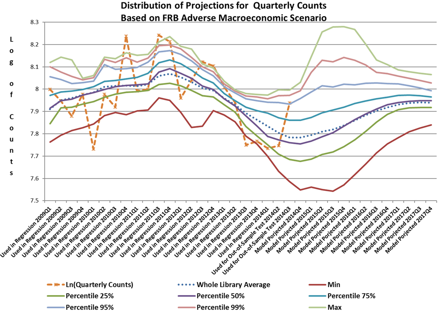
$\mathcal{L}$ - based distributions generated for the FRB Adverse Macroeconomic Scenario.

So after those reductions and applying the coefficient requirements listed in Table 5 and the model evaluating statistic requirements listed in Table 6, we built a PSRM $\mathcal{L}=(\mathcal{M},\wp)$ encompassing about 150,000 meaningful regression models. In accordance with Eq. (7), for each model $M\in\mathcal{M}$ its score was calculated by

$\displaystyle\kappa(M,\vec{w})=\sum^{8}_{i=1}w_{i}\cdot t_{i}(M),$

with the weights $w_{i},i=1,\dots,8$ as specified in Table 8.

Since the set $\mathcal{M}$ was sufficiently large, there was no need for distribution fitting similar to the one discussed in Section 2, and the Empirical Distribution Functions (EDF) yielded by PSRM $\mathcal{L}=(\mathcal{M},\wp)$ were used for the analysis required for the bank CCAR submission. Figure 5 shows an example of the distributions that were produced by $\mathcal{L}$ for the FRB Adverse Macroeconomic Scenario.

Whilst having a large model set $\mathcal{M}$ allows one to avoid uncertainty related to the distribution fitting, in some cases, dropping models with “wrong” coefficient signs and “poor” statistics might fail to reduce the model set $\mathcal{M}$ to a manageable size. One of the remedies that can be used to address the issue is the Branch and Bound Algorithm suggested in the early 1960s by Land and Doig (1960) and which is currently commonly used for discrete optimization problems (see, for example, Mehlhorn et al., 2008). This method can be effectively applied to reduce the number of regression models to a target number while assuring that the models with the “best” statistics are included in the model set $\mathcal{M}$ .

5. Conclusions

As we mentioned in Section 1, the major reason for creating and employing a PSRM is to develop a probability framework that encompasses and formalizes the model building process which is commonly employed in risk management. In practical risk management there is a significant degree of subjectivity in how models are built and which of them should be dropped or retained. Various historical periods covering different observations are commonly used in the model building process as well as lags and a variety of variable transformations (taking logarithm, applying moving averages, to mention a few). There are no universal recipes to follow or formal requirements to meet for those activities (two examples of building and using PSRMs described in Section 2 and Section 4 are illustrations.) They all are very project specific and frequently reflect expertise of the people involved.

The key idea underlying PSRM comes from the following methodological suggestion: as soon as the model building process is complete, i.e., the model set encompasses all the models that are deemed to be “meaningful,” this set can be considered to be “complete” and hence each model in this set is assigned a probability value calculated as described in Section 3. The employment of a PSRM allows one to make this subjectivity to be clearly stated and recognized (e.g., defining which statistics $\vec{S}$ are employed for model evaluation and what are the weights $\vec{w}$ used in calculating the model score $\kappa(M,\vec{w})$ .) When all decisions are made and all meaningful models are built, the PSRM allows one to see a clear probabilistic picture of what should be expected from the financial times series of interest during the projection period.

The idea of building an exhaustive (complete) space of regression models can probably be traced to the pioneering works of A. G. Ivakhnenko who introduced it in his publications dated back to the 1970s (please see Ivakhnenko and Madala, 1994). Since the recent advances in machine learning, the idea of building and working with large sets of various types of predictive models has become quite prevailing in many areas of research and practical applications including financial risk management (please see, for example, Leo et al. (2019), which includes an exhaustive list of references).

The notion of a meaningful model is commonly used in many areas of statistical research and applications and was introduced in 1980s, under the name of “intentional statistical analysis” (the reader can find a short description of it in Mandel (2014) and more details in Mandel (1988).

Assigning a probability measure to statistical models is a common feature of the Bayesian framework (see for example, George & McCulloch, 1993; George & McCulloch, 1997; and an excellent review on the subject (Fragoso & Neto, 2015)). The principal difference between the PSRM approach to calculating model’s probability and one employed in Bayesian framework is due to the absence of any prior or posterior distributions and explicit incorporation of expert opinions into the probability calculations.

Defining model probability measure as a “likelihood” that the model “will do a good job” in assessing future time development of the target variable is reminiscent to Peter L. Bernstein’s observation (Bernstein, 1998) that “In the first sense, probability means the degree of belief or approvability of an opinion – the gut view of probability.”

The author’s first attempt to explicitly incorporate model quality into developing time series projections goes back to the paper (Ladyzhets, 2012) published in 2012 where the Final House Price Model was built as a weighted average of Base Models with the weights that are proportional to Base models’ ability to estimate accurately the latest house prices. Using the terminology introduced in this paper, a Base Model is a member $M$ of the set $\mathcal{M}$ of meaningful regression model and the corresponding probability $P[M,\vec{w}]$ is defined by only one component, $w$ which is proportional to the model accuracy in estimating house prices one step ahead.

References

American Bankers Association (ABA). (March 2019). Retrieved from the association website: https://www.aba.com/Pages/default.aspx.

Basel Committee on Banking Supervision. (June 2004). International Convergence of Capital Measurement and Capital Standards, A Revised Framework. BIS.

Bernstein, P. L. (1998). Against the Gods: The Remarkable Story of Risk. Wiley.

Board of Governors of the Federal Reserve System. (February 2017). Comprehensive Capital Analysis and Review 2017 Summary Instructions for LISCC and Large and Complex Firms.

Board of Governors of the Federal Reserve System. (February 2019). 2019 Supervisory Scenarios for Annual Stress Tests Required under the Dodd-Frank Act Stress Testing Rules and the Capital Plan Rule.

Board of Governors of the Federal Reserve System. (October 2014). Comprehensive Capital Analysis and Review 2015 Summary Instructions and Guidance, Section 8.

Economic Research Division, Federal Reserve Bank of St. Louis. (March 2019). Retrieved from the Federal Reserve Bank of St. Louis website: https://fred.stlouisfed.org/series/GS10.

FedPrimeRate.com. (March 2019). Retrieved from the FedPrimeRate.com website: http://www.fedprimerate.com/mortgage_rates.htm.

Fragoso

T. M.

, & Neto

F. L.

(2015). Bayesian model averaging: A systematic review and conceptual classification. arXiv:1509.08864v1.

10.

George

E. I.

, & McCulloch

R. E.

(1993). Variable selection via Gibbs sampling. Journal of the American Statistical Association 88(423), 881-889.

11.

George

E. I.

, & McCulloch

R. E.

(1997). Approaches for Bayesian variable selection. Statistica Sinica 7(2), 339-373.

12.

Hastie

Tibshirani

, & Friedman

(2001). The Elements of Statistical Learning: Data Mining, Inference, and Prediction. Springer.

13.

Ivakhnenko

A. G.

, & Madala

H. R.

(1994). Inductive learning algorithms for complex systems modeling, CRC Press.

14.

Ladyzhets

(2012). What unemployment data can tell us about house prices: stabilizing a strong but unstable connection. in: 2012 Proceedings of the American Statistical Association, 1042-1053.

15.

Land

A. H.

, & Doig

A. G.

(1960). An automatic method of solving discrete programming problems. Econometrica, 28(3), 497-520.

16.

Leo

Sharma

, & Maddulety

(2019). Machine Learning in Banking Risk Management: A Literature Review. Risks 7(29), 1-22.

17.

Mandel

(1988). Cluster Analysis (Klasternyj analiz). Moscow: Finance and Statistics.

18.

Mandel

(2014). Three and one questions to Dr. Mirkin about complexity statistics. In Clusters, Orders, and Trees: Methods and Applications (Eds: Aleskerov, F., Goldengorin, B., & Pardalos, P.) Springer, 1-12.

19.

Mehlhorn

, & Sanders

(2008). Algorithms and Data Structures: The Basic Toolbox. Springer.

20.

Operational Riskdata eXchange Association (ORX). (March 2019). Retrieved from the association website: https://managingrisktogether.orx.org/about.

21.

Young

(1997). A Morgan Stanley Guide to Fixed Income Analysis. New York: Morgan Stanley.