Kernel-based spatial error model for analyzing spatial panel data

Abstract

Spatial panel data model captures spatial interactions across spatial units and over time. Lots of effort have been devoted to develop effective estimation methods for parametric and nonparametric spatial panel data models. Varying coefficient model has received a great deal of attention as an important tool for modeling panel data. In this paper we propose a kernel-based spatial error model for the purpose of analyzing spatial panel data. This model is based on the idea of fixed effect time-varying coefficient model and the kernel technique of support vector machine along with the technique of regularization. A generalized cross validation method is also considered for choosing the hyperparameters which affect the performance of the proposed model. The proposed model is evaluated through numerical studies.

Keywords

Fixed effect generalized cross validation kernel technique model selection spatial error model spatial panel data time-varying coefficient model

1. Introduction

When analyzing house price data, we need to consider spatial heterogeneity and spatial dependence across spatial units and over time. Spatial panel data model allows for these two specific spatial aspects of spatial house price data. The analysis of spatial panel data is a field of econometrics. For recent developments of spatial panel data models see Andrews (2010); Baltagi and Liu (2008, 2011); Debarsy and Ertur (2010); Elhorst (2003); Lee and Yu (2010a, b, c); LeSage and Pace (2009); Millo and Piras (2012); Pesaran and Tosetti (2011), and references therein.

Under the cross-sectional setting, spatial lag model (SLM) and spatial error model (SEM) deal with interactions between spatial units. The panel literature has recently considered panel regression models with spatially autocorrelated disturbances as in SEM. The fixed and random effects SEM have been recently elaborated to deal with spatial panel data like house price data with spatial and temporal variations. In general, the fixed effects model is particularly desirable when the regression analysis is limited to a precise set of subjects such as regions and firms, whereas the random effects model is more appropriate if we draw a certain number of subjects randomly from a larger population of reference (Baltagi, 2001) Varying coefficient model has recently received a great deal of attention as an important tool for modeling standard panel data (Park et al., 2015). For this reason we propose a kernel-based SEM (KBSEM) by utilizing the idea of fixed effect time-varying coefficient model and the kernel technique of support vector machine (SVM) along with the technique of regularization.

We are going to illustrate the fixed effects SEM for spatial panel data. First we need to describe the basic idea of SEM. If we try to model a spatial error process by including a proximity-weighted error term, it ends up with an SEM. The starting point of SEM is the linear cross-sectional model

$\displaystyle y_{i}=\beta_{0}+\bm{\beta}^{t}\bm{x}_{i}+\epsilon_{i},i=1,\ldots% ,n,$

where $y_{i}$ is the response variable, $\bm{x}_{i}\in R^{p}$ is a vector of covariates, $\beta_{0}$ is a unknown intercept parameter, $\bm{\beta}=(\beta_{1},\ldots,\beta_{p})^{t}\in R^{p}$ is a vector of unknown parameters, and $\epsilon_{i}$ ’s are measurement errors, which are assumed to be i.i.d. with $E(\epsilon_{i})=0$ and $\text{Var}(\epsilon_{i})=\sigma^{2}$ . The cross-sectional SEM is defined as

$\displaystyle y_{i}=\beta_{0}+\bm{\beta}^{t}\bm{x}_{i}+u_{i}$ $\displaystyle u_{i}=\rho\sum_{j=1}^{n}w_{ij}u_{j}+\epsilon_{i},|\rho|<1,i=1,% \ldots,n,$

where $\rho$ is the spatial autoregressive parameter and $\epsilon_{i}$ ’s are assumed to be i.i.d. with $E(\epsilon_{i})=0$ and $\text{Var}(\epsilon_{i})=\sigma^{2}$ .

The standard fixed effects model for panel data is

$\displaystyle y_{ij}=\beta_{0}+\bm{\beta}^{t}\bm{x}_{ij}+\mu_{i}+\epsilon_{ij}% ,i=1,\ldots,m,j=1,\ldots,n,$

where $i$ is an index for the cross-sectional dimension, $j$ is an index for the time dimension, $y_{ij}$ is the response variable, $\bm{x}_{ij}\in R^{p}$ is a vector of covariates, $\beta_{0}$ is a unknown intercept parameter, $\bm{\beta}=(\beta_{1},\ldots,\beta_{p})^{t}\in R^{p}$ is a vector of unknown parameters, $\mu_{i}$ reflects the unobserved subject effect such that $\sum_{i=1}^{m}\mu_{i}=0$ , and $\epsilon_{ij}$ ’s are idiosyncratic errors. For simplicity we consider the balanced case. The SEM for spatial panel data introduces fixed effects or random effects. The fixed effects SEM is defined as

$\displaystyle y_{ij}=\beta_{0}+\bm{\beta}^{t}\bm{x}_{ij}+\mu_{i}+u_{ij}$ (1) $\displaystyle u_{ij}=\rho\sum_{k=1}^{m}w_{ik}u_{kj}+\epsilon_{ij},|\rho|<1,$

where $w_{ik}$ is an element of an $m\times m$ spatial weights matrix $\bm{W}_{m}$ describing the spatial arrangement of the subjects in the sample, and $\epsilon_{ij}$ ’s assumed to be i.i.d. with $E(\epsilon_{ij})=0$ and $\text{Var}(\epsilon_{ij})=\sigma^{2}$ . The elements of $\bm{W}_{m}$ are standardized such that the elements in each row sum to 1. To utilize it later we rewrite the fixed effects SEM (1) in a matrix notation as follows:

$\displaystyle\bm{y}=(\bm{1}_{n}\otimes\bm{I}_{m})\bm{\mu}+\bm{X}\bm{\beta}+\bm% {u}$ (2) $\displaystyle\bm{u}=\rho(\bm{I}_{n}\otimes\bm{W}_{m})\bm{u}+\bm{\epsilon},{\rm i% .e.},\bm{u}=(\bm{I}_{N}-\rho(\bm{I}_{n}\otimes\bm{W}_{m}))^{-1}\bm{\epsilon},$

where $\otimes$ represents the Kronecker product, $N=mn$ , $\bm{1}_{d}$ is a vector of ones of dimension $d$ , $\bm{I}_{d}$ is an identity matrix of dimension $d$ , $\bm{W}_{m}$ is an $m\times m$ spatial weights matrix, $\bm{y}=(y_{11},\ldots,y_{1n},\ldots,y_{m1},\ldots,y_{mn})^{t}$ , $\bm{\mu}=(\mu_{1},\ldots,\mu_{m})^{t}$ , $\bm{\beta}=(\beta_{0},\beta_{1},\ldots,\beta_{p})^{t}$ , $\bm{X}=(\bm{1}_{N},\bm{X}_{0})$ is $N\times(p+1)$ matrix with $\bm{X}_{0}=(\bm{x}_{11},\ldots,\bm{x}_{1n},\ldots,\bm{x}_{m1},\ldots,\bm{x}_{% mn})^{t}$ , $\bm{u}=(u_{11},\ldots,u_{1n},\ldots,u_{m1},\ldots,u_{mn})^{t}$ , and $\bm{\epsilon}=(\epsilon_{11},\ldots,\epsilon_{1n},\ldots,\epsilon_{m1},\ldots,% \epsilon_{mn})^{t}$ .

For panel data Li et al. (2015) considered the following time-varying coefficients model (TVCM).

$\displaystyle y_{ij}=\beta_{0}(t_{ij})+\bm{\beta}(t_{ij})^{t}\bm{x}_{ij}+\mu_{% i}+\epsilon_{ij},i=1,\ldots,m,j=1,\ldots,n_{i},$ (3)

where $t_{ij}$ is the time of the $j$ th observation for the $i$ th subject, $\beta_{0}(t_{ij})$ represents the baseline effect, $\bm{\beta}(t_{ij})=(\beta_{1}(t_{ij}),\ldots,\beta_{p}(t_{ij}))^{t}$ , $\mu_{i}$ reflects the unobserved subject effect, and $\epsilon_{ij}$ is independent of $\mu_{i}$ and $\bm{x}_{ij}\in R^{p}$ . Here, $\mu_{i}$ is time-invariant and it accounts for the subject’s unobserved ability. Model (3) is called as a fixed effects TVCM when $\mu_{i}$ is allowed to be correlated with $\bm{x}_{ij}$ . For identification purpose, we impose the restriction for the fixed effects model that $\sum_{i=1}^{m}\mu_{i}=0$ .

For analysis of spatial panel data we are going to propose the KBSEM using the kernel technique of SVM firstly developed by Vapnik (1995) and his group at AT&T Bell Laboratories. To the best of our knowledge, the VC approach has not been applied to SEM for modeling spatial panel data. The rest of this paper is organized as follows. Section 2 describes the KBSEM along with its model selection procedure. Section 3 and Section 4 present numerical studies and conclusion, respectively.

2. The proposed KBSEM

In this section we illustrate KBSEM with estimation and model selection procedures. The KBSEM is derived by applying spatial error term and the kernel technique of SVM to the TVCM (3) with fixed effects. We consider the balanced case $n=n_{i}$ .

2.1 Estimation procedure

Given the training data set ${\mathcal{D}}=\{(t_{ij},\bm{x}_{ij},y_{ij})\}_{i,j=1}^{m,n}$ , we first consider a fixed effects TVCM of the form

$\displaystyle y_{ij}=f(t_{ij},\bm{x}_{ij})+u_{ij}=\bm{\beta}(t_{ij})^{t}\bm{x}% _{ij}+{\mu}_{i}+u_{ij},u_{ij}=\rho\sum_{k=1}^{m}w_{ik}u_{kj}+\epsilon_{ij},$ (4)

where $\mu_{i}$ reflects the unobserved subject effect such that $\sum_{i=1}^{m}\mu_{i}=0$ , $\bm{x}_{ij}=(1,x_{ij1},\ldots,x_{ijp})^{t}$ , $\bm{\beta}(t_{ij})=(\beta_{0}(t_{ij}),\beta_{1}(t_{ij}),\ldots,\beta_{p}(t_{ij% }))^{t}$ , and $\epsilon_{ij}$ ’s are idiosyncratic errors.

We now assume that coefficient function $\beta_{k}(t_{ij})$ in the model (4) for $k=0,1,\ldots,p$ is nonlinearly related to time $t_{ij}$ such that $\beta_{k}(t_{ij})=\bm{w}_{k}^{t}\bm{\phi}(t_{ij})+b_{k}$ where $\bm{w}_{k}$ is a corresponding $d_{\rm f}\times 1$ weight vector to $\bm{\phi}(t_{ij})$ . Here the nonlinear feature mapping function $\bm{\phi}:R\rightarrow R^{d_{f}}$ maps the input space to the higher dimensional feature space where the dimension $d_{f}$ is defined in an implicit way. An inner product in feature space has an equivalent kernel in input space, $K(t_{ij},t_{\rm uv})=\bm{\phi}(t_{ij})^{t}\bm{\phi}(t_{\rm uv})$ , provided certain conditions hold (Mercer, 1909). Several choices of the kernel function are possible. One popular choice of kernel function in practice is Gaussian kernel defined as

$\displaystyle K(t_{ij},t_{\rm uv})=\exp(-(t_{ij}-t_{\rm uv})^{2}/2\kappa),$

where $\kappa>0$ is prespecified kernel parameter.

We consider the nonlinear case, in which the regression function given $(t_{ij},\bm{x}_{ij})$ , can be regarded as a nonlinear function of $t_{ij}$ as follows:

$\displaystyle f(t_{ij},\bm{x}_{ij})=\sum_{k=0}^{p}x_{ijk}(\bm{w}_{k}^{t}\bm{% \phi}(t_{ij})+b_{k})+{\mu}_{i},\sum_{i=1}^{m}{\mu}_{i}=0.$ (5)

With the weighted quadratic loss with regard to error term $\bm{u}$ in Eq. (5) we define the optimization problem

$\displaystyle\min_{\bm{w}_{k},b_{k},\epsilon_{ij}}\frac{1}{2}\sum_{k=0}^{p}\|% \bm{w}_{k}\|^{2}+\frac{\lambda}{2}{\bm{u}}^{t}(\bm{I}_{N}-\rho\bm{W})^{t}(\bm{% I}_{N}-\rho\bm{W})\bm{u}$ (6)

subject to constraints

$\displaystyle y_{ij}=\sum_{k=0}^{p}x_{ijk}(\bm{w}_{k}^{t}\bm{\phi}(t_{ij})+b_{% k})+\mu_{i}+u_{ij}\text{and}\sum_{i=1}^{m}{\mu}_{i}=0,$

where $\lambda$ is penalty parameter and $\bm{W}=\bm{I}_{n}\otimes\bm{W}_{m}$ .

Then, by writing the constraints of the optimization problem (5) in a matrix notation, we can construct Lagrangian function for fixed $\rho$ as

$\displaystyle L=\frac{1}{2}\sum_{k=0}^{p}\|\bm{w}_{k}\|^{2}+\frac{\lambda}{2}{% \bm{u}}^{t}(\bm{I}_{N}-\rho\bm{W})^{t}(\bm{I}_{N}-\rho\bm{W})\bm{u}+\bm{\alpha% }^{t}(\bm{y}-\sum_{k=0}^{p}\bm{X}_{k}(\bm{\Phi}\bm{w}_{k}+\bm{1}_{N}b_{k})-\bm% {B}\bm{\mu}_{1}-\bm{u}),$ (7)

where $\bm{\alpha}=(\alpha_{11},\ldots,\alpha_{1n},\ldots,\alpha_{m1},\ldots,\alpha_{% mn})^{t}$ , $\bm{X}_{k}=\text{diag}\{x_{11k},\ldots,x_{1nk},\ldots,$ $x_{m1k},\ldots,x_{mnk}\}$ , $\bm{\Phi}=(\bm{\phi}(t_{11}),\ldots,\bm{\phi}(t_{1n}),\ldots,\bm{\phi}(t_{m1})% ,\ldots,\bm{\phi}(t_{mn}))^{t}$ , $\bm{\mu}_{1}=(\mu_{1},\ldots,\mu_{m-1})^{t}$ , and $\bm{B}=(\bm{B}_{1}^{t},\bm{B}_{2}^{t})^{t}$ is $N\times(m-1)$ matrix with $(m-1)n\times(m-1)$ block diagonal matrix $\bm{B}_{1}=\text{diag}\{\bm{1}_{n},\ldots,\bm{1}_{n}\}$ and $n\times(m-1)$ matrix $\bm{B}_{2}=(-\bm{1}_{n},\ldots,-\bm{1}_{n})$ . Here, $\bm{B}\bm{\mu}_{1}$ in Eq. (7) reflects the constraint $\sum_{i=1}^{m}\mu_{i}=0$ .

From the optimality conditions, we can get the followings:

$\displaystyle\frac{\partial L}{\partial\bm{w}_{k}}={\bf 0}_{d_{f}}\Rightarrow% \bm{w}_{k}=\bm{\Phi}^{t}\bm{X}_{k}\bm{\alpha}$ $\displaystyle\frac{\partial L}{\partial b_{k}}=0\Rightarrow\bm{\alpha}^{t}\bm{% X}_{k}\bm{1}_{N}=0,k=0,1,\ldots,p$ $\displaystyle\frac{\partial L}{\partial\bm{\mu}_{1}}=\textbf{0}_{m-1}% \Rightarrow\bm{B}^{t}\bm{\alpha}=\bm{0}_{m-1}$ $\displaystyle\frac{\partial L}{\partial\bm{\alpha}}=\bm{0}_{N}\Rightarrow\bm{y% }-\sum_{k=0}^{p}\bm{X}_{k}(\bm{\Phi}\bm{w}_{k}+b_{k}\bm{1}_{N})-\bm{B}\bm{\mu}% _{1}-\bm{u}=\bm{0}_{N}$ $\displaystyle\frac{\partial L}{\partial\bm{u}}={\bf 0}_{N}\Rightarrow\bm{u}=% \frac{1}{\lambda}[(\bm{I}_{N}-\rho\bm{W})^{t}(\bm{I}_{N}-\rho\bm{W})]^{-1}\bm{\alpha}$

where $\bm{0}_{d}$ is a vector of zeroes of dimension $d$ .

After eliminating $\bm{u}$ and $\bm{w}_{k}$ ’s, we have the optimal values $\hat{\bm{\alpha}}$ , $\hat{\bm{b}}$ and $\hat{\bm{\mu}}_{1}$ which are obtained from the linear equation as follows:

$\displaystyle\begin{pmatrix}\bm{Z}&\bm{X}&\bm{B}\\ \bm{X}^{t}&\bm{O}_{1}&\bm{O}_{2}\\ \bm{B}^{t}&\bm{O}_{2}^{t}&\bm{O}_{3}\end{pmatrix}\begin{pmatrix}\bm{\alpha}\\ \bm{b}\\ \bm{\mu}_{1}\end{pmatrix}=\begin{pmatrix}\bm{y}\\ \bm{0}_{p+1}\\ \bm{0}_{m-1}\end{pmatrix},$ (8)

where $\bm{Z}=(\bm{X}\bm{X}^{t})\odot\bm{K}+\frac{1}{\lambda}[(\bm{I}_{N}-\rho\bm{W})% ^{t}(\bm{I}_{N}-\rho\bm{W})]^{-1}$ with the $N\times(p+1)$ matrix $\bm{X}=(\bm{1}_{N},\bm{X}_{0})$ and the $N\times N$ kernel matrix $\bm{K}$ consisting of $K(t_{ik},t_{il}),i=1,\ldots,m,k,l=1,\ldots,n$ , $\bm{b}=(b_{0},b_{1},\ldots,b_{p})^{t}$ , $\bm{O}_{1}$ is the $(p+1)\times(p+1)$ zero matrix, $\bm{O}_{2}$ is the $(p+1)\times(m-1)$ zero matrix, and $\bm{O}_{3}$ is the $(m-1)\times(m-1)$ zero matrix. Here $\odot$ denotes a componentwise multiplication.

For a point $(t_{st},\bm{x}_{st}),s=1,\ldots,m$ , the estimator of $\beta_{k}(t_{st})$ takes the form:

$\displaystyle\hat{\beta}_{k}(t_{st})=\sum_{i=1}^{m}\sum_{j=1}^{n}x_{ijk}K(t_{% st},t_{ij})\hat{\alpha}_{ij}+\hat{b}_{k},k=0,1,\ldots,p,$ (9)

and then the estimator of regression function takes the form:

$\displaystyle\hat{f}(t_{st},\bm{x}_{st})=\begin{cases}\displaystyle\sum_{k=0}^% {p}x_{stk}\hat{\beta}_{k}(t_{st})+\hat{\mu}_{\rm s}&\text{if }s\neq m\\ \displaystyle\sum_{k=0}^{p}x_{stk}\hat{\beta}_{k}(t_{st})-\sum_{i=1}^{m-1}\hat% {\mu}_{i}&\text{if }s=m\end{cases}$ (10)

We remark that $(t_{st},\bm{x}_{st})$ could be an observation in the training data set ${\mathcal{D}}$ or a new observation. In particular, for any $(t_{st},\bm{x}_{st})\in{\mathcal{D}}$ we can express the estimator Eq. (10) as follows:

$\displaystyle\hat{f}(t_{st},\bm{x}_{st})=\bm{h}_{st}\bm{y},$

where $\bm{h}_{st}=(((1,\bm{x}_{st}^{t})\bm{X}^{t})\odot\bm{k}_{st},(1,\bm{x}_{st}^{t% })^{t},\bm{b}_{\rm s})\bm{H}_{0}$ , $\bm{b}_{\rm s}$ is a row of $\bm{B}$ corresponding to the $s$ th region, $\bm{k}_{st}$ is the $1\times N$ kernel vector consisting of $K(t_{\rm ts},t_{ik}),i=1,\ldots,m,k=1,\ldots,n$ , and $\bm{H}_{0}$ is defined as

$\displaystyle\bm{H}_{0}=\begin{pmatrix}\bm{Z}^{-1}-\bm{Z}^{-1}\bm{Z}_{1}(\bm{Z% }_{1}^{t}\bm{Z}^{-1}\bm{Z}_{1})^{-1}\bm{Z}_{1}^{t}\bm{Z}^{-1}\\ (\bm{Z}_{1}^{t}\bm{Z}^{-1}\bm{Z}_{1})^{-1}\bm{Z}_{1}^{t}\bm{Z}^{-1}\end{pmatrix}$ (11)

with $\bm{Z}_{1}=(\bm{X},\bm{B})$ .

The solution to Eq. (8) cannot be obtained in a single step since unknown $\rho$ is involved. Thus we need to apply an iterative procedure which starts with initialized values of $\rho$ . We describe an iterative procedure for the simultaneous estimation of $(\hat{\bm{\alpha}},\hat{\bm{b}},\hat{\bm{\mu}}_{1})$ and $\rho$ for given hyperparameters as follows:

Start with the initial value $\rho=0$ .

Calculate the solutions, $\hat{\bm{\alpha}},\hat{\bm{b}}$ and $\hat{\bm{\mu}}_{1}$ , of the linear equation Eq. (8) using the estimates $\rho$ obtained in the previous step.

Using $\hat{\bm{\alpha}},\hat{\bm{b}}$ and $\hat{\bm{\mu}}_{1}$ obtained in the previous step, calculate the estimates $\hat{\rho}$ as follows:

$\displaystyle\hat{\rho}=\frac{\hat{\bm{u}}\bm{W}^{t}\hat{\bm{u}}}{\hat{\bm{u}}% \bm{W}^{t}\bm{W}\hat{\bm{u}}},$

where $\hat{\bm{u}}$ is $N\times 1$ vector consisting of $\hat{u}_{ij}=y_{ij}-\hat{f}(t_{ij},\bm{x}_{ij}),i=1,\ldots,m,j=1,\ldots,n$ .

Iterate steps 2 and 3 until convergence.

The estimation procedure is iterated until the following stop criterion is satisfied:

$\displaystyle\frac{1}{N}\|\hat{\bm{\alpha}}^{(k)}-\hat{\bm{\alpha}}^{(k+1)}\|^% {2}<\epsilon,$

where the superscript $k$ denotes the $k$ th iteration. Here we take $\epsilon=10^{-6}$ as the tolerance level. The algorithm converges somewhat fast according to our experience.

2.2 Model selection

We now consider the model selection problem which determines the appropriate hyperparameters of the proposed KBSEM for spatial panel data. The functional structure of the proposed model is characterized by hyperparameters such as the regularization parameters $\lambda$ and the kernel parameter $\kappa$ . To choose the values of hyperparameters of the proposed model we first need to consider the cross validation (CV) function as follows:

$\displaystyle CV(\bm{\lambda})=\frac{1}{N}\sum_{i=1}^{m}\sum_{j=1}^{n}(y_{ij}-% {\hat{f}}^{(-ij)}(t_{ij},\bm{x}_{ij}|\bm{\lambda}))^{2},$

where $\bm{\lambda}$ is the set of hyperparameters, and $\hat{f}^{(-ij)}(t_{ij},\bm{x}_{ij}|\bm{\lambda})$ is the regression function estimated without $j$ th observation of $i$ th subject.

But the computational cost associated with CV function is formidable since $\hat{f}^{(-ij)}(t_{ij},\bm{x}_{ij}|\bm{\lambda})$ should be evaluated for each candidate set of hyperparameters. By leaving-out-one lemma (Craven & Wahba, 1979),

$\displaystyle({y}_{ij}-\hat{f}^{(-ij)}(t_{ij},\bm{x}_{ij}|\bm{\lambda}))-(y_{% ij}-\hat{f}(t_{ij},\bm{x}_{ij}|\bm{\lambda}))=\hat{f}(t_{ij},\bm{x}_{ij}|\bm{% \lambda})-\hat{f}^{(-ij)}(t_{ij},\bm{x}_{ij}|\bm{\lambda})$ $\displaystyle\simeq\frac{\partial\hat{f}(t_{ij},\bm{x}_{ij}|\bm{\lambda})}{% \partial y_{ij}}(y_{ij}-\hat{f}^{(-ij)}(t_{ij},\bm{x}_{ij}|\bm{\lambda})),$

we have

$\displaystyle(y_{i}-\hat{f}^{(-ij)}(t_{ij},\bm{x}_{ij}|\bm{\lambda}))\simeq% \frac{y_{ij}-\hat{f}(t_{ij},\bm{x}_{ij}|\bm{\lambda})}{1-{\displaystyle\frac{% \partial\hat{f}(t_{ij},\bm{x}_{ij}|\bm{\lambda})}{\partial y_{ij}}}}.$

Then the ordinary cross validation (OCV) function can be obtained as

$\displaystyle OCV({\bm{\lambda}})=\frac{1}{N}\sum_{i=1}^{m}\sum_{j=1}^{n}\left% (\frac{y_{ij}-{\hat{f}}(t_{ij},\bm{x}_{ij}|\bm{\lambda})}{1-{\displaystyle% \frac{\partial\hat{f}(t_{ij},\bm{x}_{ij}|\bm{\lambda})}{\partial y_{ij}}}}% \right)^{2}.$

Thus, the generalized cross validation (GCV) function can be obtained as

$\displaystyle GCV(\bm{\lambda})=\frac{N\bm{y}^{t}(\bm{I}_{N}-\bm{H})^{t}(\bm{I% }_{N}-\bm{H})\bm{y}}{(N-{\rm tr}(\bm{H}))^{2}}.$ (12)

In fact, this GCV function Eq. (11) is utilized when determining the optimal value of $\bm{\lambda}$ . Here $\bm{H}$ is the hat matrix such that

$\displaystyle\hat{\bm{f}}\equiv({\hat{f}}(t_{11},\bm{x}_{11}|\bm{\lambda}),% \ldots,{\hat{f}}(t_{mn},\bm{x}_{mn}|\bm{\lambda}))^{t}=\bm{H}\bm{y},$

where the $i j$ th element of $\bm{H}$ is $h_{ij}=\frac{\partial{\hat{f}}(t_{ij},\bm{x}_{ij}|\bm{\lambda})}{\partial y_{% ij}}$ . In fact, $\bm{H}$ turns out to be equal to

$\displaystyle\bm{H}=((\bm{X}\bm{X}^{t})\odot\bm{K},\bm{X},\bm{B})\bm{H}_{0},$

where $\bm{H}_{0}$ is given Eq. (11).

3. Numerical studies

In this section we investigate the estimation performance of the KBSEM for one synthetic example and one real example related to analyzing house price data. In these examples we compare the KBSEM with a spatial panel fixed effects model (SPFEM). The estimation of the SPFEM is performed by using splm module in R package. Throughout the paper, to determine the optimal parameters of the KBSEM we use the corresponding GCV function.

3.1 Synthetic example

In this example we conduct the simulation study on the efficacy of the proposed KBSEM, and compare our model with SPFEM. We use the following data generating process:

$\displaystyle y_{ij}=\beta_{0}(t_{ij})+\beta_{1}(t_{ij})x_{ij1}+\beta_{2}(t_{% ij})x_{ij2}+\mu_{i}+u_{ij}$ $\displaystyle u_{ij}=\rho\sum_{k=1}^{m}w_{ik}u_{kj}+\epsilon_{ij},i=1,\ldots,m% ,j=1,\ldots,n$

where $\beta_{0}(t_{ij})=\sin(0.5t_{ij}/\pi)+\cos(0.5t_{ij}/\pi)$ , $\beta_{1}(t_{ij})=\sin(0.5t_{ij}/\pi)$ , $\beta_{2}(t_{ij})=\cos(0.5t_{ij}/\pi)$ , $t_{ij}=j$ , $\rho=0.36$ , $x_{ij1}\sim U(0,2)$ , $x_{ij2}\sim U(0,2)$ , $\mu_{i}\sim N(0,1)$ and $\epsilon_{ij}\sim N(0,0.5^{2})$ . We set $m$ equal to 8 and $n$ to 20. Further, the elements $w_{ik}$ of the spatial weights matrix are obtained from the map in Fig. 1.

Table 1
Performance comparison of the proposed KBSEM and SPFEM for the synthetic example (standard error in parenthesis)

Data type	KBSEM	SPFEM
Training data	0.3004 (0.0414)	3.4963 (0.0913)
Test data	1.0572 (0.0413)	3.5194 (0.0919)

Figure 1.

The synthetic region map.

For this example we generate 50 training and 50 test data sets. For each training data set and test data set we compute MSE with regard to $f_{ij}=\beta_{0}(t_{ij})+\beta_{1}(t_{ij})x_{ij1}+\beta_{2}(t_{ij})x_{ij2}+\mu% _{i}$ . The results are reported in Table 1, which describes the proposed KBSEM yields the smaller means of MSEs for both training and test data. The test statistics and $p$ -values associated with two sample $t$ -test for a null hypothesis that the mean of MSEs of the KBSEM is equal to that of SPFEM are obtained as 55.5535 (0.0) and 74.3936 (0.0), respectively for training and test data sets. The relevant $p$ -values are given in parenthesis. We observe that the means of MSEs of KBSEM are significantly smaller than those of SPFEM for both training and test data. Thus we conclude that the proposed KBSEM shows the better fitting performance and the better generalization performance for this synthetic example.

3.2 Hedonic house price example

3.2.1 Data explanation

In order to estimate the hedonic house price function of the US, we set up 48 states and District of Columbia (DC) of the United States of America as targeting areas. At this, the reason that we restrict 48 states out of total 50 states is only because Alaska (AK) and Hawaii (HI) are located apart and noncontiguous from the main land of the US. We collect the data from various sources. First of all, we use housing price index (HPI) from Federal Housing Finance Agency as a dependent variable. According to Federal Housing Finance Agency, this data is broadly measured from the repeat sale prices average of single-family house prices, so that it seems to have sufficient representativeness for the movement of housing sale prices of the US.

On the other hand, we collect data focusing on the variables empirically proven by large literatures. At this, we only include collectable variables with panel data format out of the entire candidate variables. To begin with, it is well known that GDP or income are closely related to housing market (Davis & Heathcote, 2005; Iacoviello & Neri, 2010; Goodhart & Hofmann, 2008; Adams & Füss, 2010). In this regard, we use GDP in current dollars from Bureau of Economic Analysis and median household income by state (denoted as INCOME) from United States Census Bureau as independent variables. Besides, interest is also a well-known factor for determination of housing prices: especially, negative relationship. This is because rise of interest can make lessen the financing ability of the prospective buyers, so this explains that interest and housing prices are negatively related (Apergis & Rezitis, 2003; Anselin et al., 2010; Igan et al., 2011). In this context, this research uses mortgage interest rate (MIR) from Federal Housing Finance Agency as an another independent variable for estimating HPI.

Lastly, employment also functions as an important factor for the real estate activity of individuals (Lerbs, 2011; Giussani et al., 1993; Baffoe-Bonnie, 1998). Therefore, we set up employment status of the civilian noninstitutional population (denoted as EMP) from Bureau of Labor Statistics as the fourth independent variable. In regard of obtaining data, we set up time period from 1991 to 2015 in which data can be annually collected as many as possible. While there are only missing data on MIR in Oklahoma (OK) period 2005–2008 out of entire panel data. Hence, we fill in the missing data with the average value between 2004 and 2009 MIR values.

3.2.2 Estimation results

We now investigate the estimation performance of the KBSEM for house sales price data, for which the repeat sale prices average of single-family house prices is recorded from 1991 to 2015 in 48 states and District of Columbia (DC) of the United States of America. We now consider the parametric and nonparametric specifications for the hedonic price function and the estimation procedures. We compare the KBSEM with the SPFEM in terms of estimating regression function and fixed effects. We also report the estimation results for varying coefficient functions. For analysis, each independent variable and time variable are standardized using $(x-\min(x))/(\max(x)-\min(x))$ .

Table 2
Definition and description of the variables for house sales price data

Variable	Description
HPI	Housing price index
GDP	GDP in current dollars
INCOME	Median household income by state
MIR	Mortgage interest rate
EMP	Employment status of the civilian noninstitutional population

Let $\bm{x}$ and $y$ represent a vector of four independent variables and dependent variable, respectively. The SPFEM for this house price data is

$\displaystyle\log(y_{ij})=\beta_{0}+\sum_{k=1}^{4}\beta_{k}x_{ijk}+\mu_{i}+u_{% ij},$ $\displaystyle u_{ij}=\rho\sum_{k=1}^{49}w_{ik}u_{kj}+\epsilon_{ij},\sum_{i=1}^% {49}\mu_{i}=0,$

where $\epsilon_{ij}\sim\text{i.i.d.}N(0,\sigma^{2})$ for $i=1,\ldots,49,j=1,\ldots,14$ . Note that $m=49$ and $n=14$ for house price data. The KBSEM for this house price data is

$\displaystyle\log(y_{ij})=\beta_{0}(t_{ij})+\sum_{k=1}^{4}\beta_{k}(t_{ij})x_{% ijk}+\mu_{i}+u_{ij}$ $\displaystyle u_{ij}=\rho\sum_{k=1}^{49}w_{ik}u_{kj}+\epsilon_{ij},\sum_{i=1}^% {49}\mu_{i}=0,$

where $\epsilon_{ij}\sim\text{i.i.d.}N(0,\sigma^{2})$ for $i=1,\ldots,49,j=1,\ldots,14$ .

First we develop the SPFEM using the given data, which is then used to investigate estimation performance. The regression equation representing the average relationships of the spatial units between the level of housing price and four factors is presented in Table 3. We also examine MSE with regard to $\log(y_{ij})$ and $\hat{\log(y_{ij})}$ for the given data set. The MSE is defined as

$\displaystyle\frac{1}{49\times 14}\sum_{i=1}^{49}\sum_{j=1}^{14}(\log(y_{ij})-% \hat{\log(y_{ij})})^{2}.$

The value of MSE of the SPFEM is 0.0752. These results indicate that the assessed house values can be modeled by the selected four variables. Therefore, the hypothesized relationships between the independent variables and the house values are supported by the data. Indeed, GDP, INCOME and EMP determinants are statistically significant at 95% confidence level according to their $t$ -probabilities. In particular, GDP, median household income and employment status are positively associated with house values, whereas mortgage interest rate is negatively associated with the house values. The estimated value of the spatial parameter $\rho$ is 0.6497 and turns out to be statistically significant at 95% confidence level according to their $t$ -probabilities. This indicates the relative importance of the spatial context to the model.

Table 3

Hedonic model (SPFEM) parameter estimate summaries

	Estimate	Std. error	$t$ -statistic	$t$ -probability
Intercept	4.8006	0.0303	158.3800	2.2e-16
GDP	0.6939	0.0644	10.7698	2.2e-16
INCOME	0.3886	0.0679	5.7250	1.034e-08
MIR	$-$ 0.0136	0.0555	$-$ 0.2454	0.8062
EMP	0.2297	0.0696	3.3001	0.00097
$\rho$	0.6497	0.0311	20.9031	2.2e-16

Table 4

Hedonic model (KBSEM) parameter estimate summaries

$\beta_{0}$	$\beta_{1}$	$\beta_{2}$	$\beta_{3}$	$\beta_{4}$
4.7973	0.9951	0.3081	$-$ 0.2643	0.3220
(0.0474)	(0.1156)	(0.0366)	(0.0797)	(0.0425)

Figure 2.

The estimated 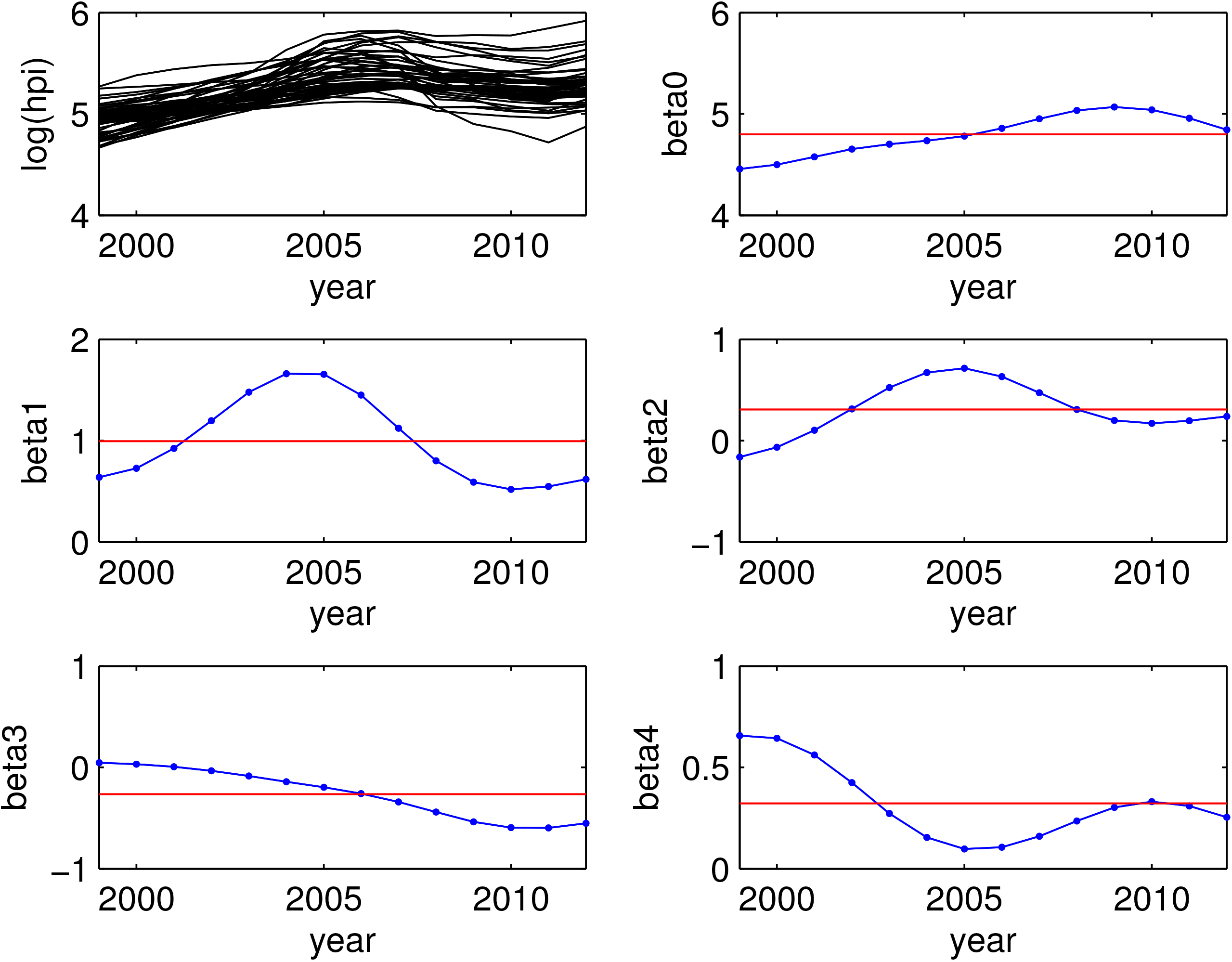$\log(hpi)$ and estimated coefficient functions by KBSEM.

We now develop the KBSEM using the given data. The values of hyperparameters $(\lambda,\kappa)$ are determined by GCV function Eq. (12) as $(20,0.1)$ in this case study. The estimation results for $\beta_{k}$ ’s are shown in Table 4. Table 4 presents averages and standard errors of the estimated values for $\beta_{k}$ ’s. Standard errors are given in parenthesis. Here, the estimated values for $\beta_{k}$ ’s are obtained by Eq. (9), and the standard errors are computed using the jackknife method. These values show the pattern similar to those for the SPFEM in terms of size and sign. The estimated value of the spatial parameter $\rho$ is 0.5787. The value of MSE of the KBSEM is 0.0044, which is much smaller than the value of MSE of the SPFEM. This implies that the KBSEM performs better than the SPFEM in estimating regression function. Figure 2 depicts the estimated coefficient functions obtained by the KBSEM. The red line indicates the average of the estimated values over time of each coefficient function $\beta_{k}$ . The blue curve indicates the estimated coefficient function. From the estimated coefficient functions, we can see they have different degrees of smoothness for this data set. Figure 2describes the extent to which the coefficients vary with time. Figure 2 shows that the smoothing variable time gives strong effect on the regression coefficients. Figure 3 depicts the estimated values of spatial specific effects $\mu_{i}$ ’s obtained by SPFEM and KBSEM.

Figure 3.

The estimated values of spatial specific effects $\mu_{i}$ ’s obtained by SPFEM (left panel) and KBSEM (right panel).

4. Conclusions

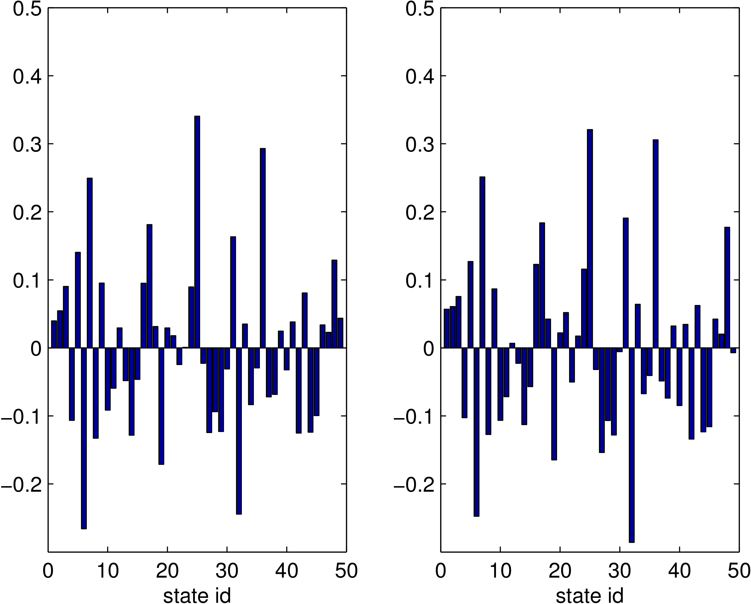
In this paper we proposed the KBSEM to account for spatial interactions across spatial units and over time that exist in the house prices. The underlying idea of the proposed KBSEM is that SEM is approximated by a combination of linear least squares SVM (LS-SVM) and nonlinear feature mapping function of the coordinate $t_{ij}$ . The limitation of the KBSEM is that it constrains on balanced data case for the time observation. An application to estimating the hedonic house price function of the United States of America is used to provide support for the case which we make for the SEM.

This paper analyzed data incorporating spatial effects through error term and reflecting spatial interactions of house prices across spatial units and over time. The SPFEM and KBSEM used in the study were built based on synthetic data and house price data collected from 1991 to 2015 in 48 states and District of Columbia (DC) of the United States of America. The performances of these models were then compared based on MSE. This paper demonstrates that the proposed KBSEM provides good results in goodness of fit for the given two examples. To conclude, we proposed a more efficient KBSEM to capture spatial interactions across spatial units and over time.

Footnotes

Acknowledgments

This research was supported by Basic Science Research Program through the National Research Foundation of Korea (NRF) funded by the Ministry of Education, Science and Technology with grant no. (NRF-2018R1D1A1B07042349). This research was supported by the Bio & Medical Technology Development Program of the National Research Foundation (NRF) funded by the Korean government (MSIT) (No. 2019M3E5D4066897). This research was supported by the Human Resources Program in Energy Technology of the Korea Institute of Energy Technology Evaluation and Planning (KETEP) granted financial resource from the Ministry of Trade, Industry & Energy, Republic of Korea (No. 20174030201740).

References

Adams

, & Füss

(2010). Macroeconomic determinants of international housing markets. Journal of Housing Economics, 19, 38-50.

Andrews

(2010). Real house prices in OECD Countries: The role of demand shocks and structural and policy factors. OECD Publishing.

Anselin

Gallo

J. L.

, & Jayet

(2008). Spatial panel econometrics. In: Matyas

Sevestre

(eds), The Econometrics of Panel Data. Springer-Verlag, Berlin Heidelberg, 625-660.

Apergis

, & Rezitis

(2003). Housing prices and macroeconomic factors in Greece: Prospects within the EMU. Applied Economics Letters, 10, 799-804.

Baffoe-Bonnie

(1998). The dynamic impact of macroeconomic aggregates on housing prices and stock of houses. Journal of Real Estate Finance & Economics, 17, 179-197.

Baltagi

B. H.

(2001). Econometric analysis of panel data. Wiley, Chichester.

Baltagi

B. H.

, & Liu

(2008). Testing for random effects and spatial lag dependence in panel data models. Statistics & Probability Letters, 78, 3304-3306.

Baltagi

B. H.

, & Liu

(2011). Instrumental variable estimation of a spatial autoregressive panel model with random effects. Economics Letters, 111, 135-137.

Craven

, & Wahba

(1979). Smoothing noisy data with spline functions: Estimating the correct degree of smoothing by the method of generalized cross-validation. Numerical Mathematics, 31, 377-403.

10.

Davis

, & Heathcote

(2005). Housing and the business cycle. International Economic Review, 46, 751-784.

11.

Debarsy

, & Ertur

(2010). Testing for spatial autocorrelation in a fixed effects panel data model. Regional Science and Urban Economics, 40, 453-470.

12.

Elhorst

J. P.

(2003). Specication and estimation of spatial panel data models. International Regional Sciences Review, 26, 244-268.

13.

Elhorst

J. P.

(2008). Serial and spatial error correlation. Economics Letters, 100, 422-424.

14.

Elhorst

J. P.

(2010). Dynamic panels with endogenous interactions effects when t is small. Regional Science and Urban Economics, 40, 272-282.

15.

Giussani

Hsia

, & Tsolacos

(1993). A comparative analysis of the major determinants of office rental values in Europe. Journal of Property Valuation and Investment, 11, 157-173.

16.

Goodhart

, & Hofmann

(2008). House prices, money, credit, and the macroeconomy. Oxford Review of Economic Policy, 24, 180-205.

17.

Iacoviello

, & Neri

(2010). Housing market spillovers: Evidence from an estimated DSGE model. American Economic Journal: Macroeconomics, 2, 125-164.

18.

Igan

Kabundi

De Simone

F. N.

Pinheiro

, & Tamirisa

(2011). Housing, credit, and real activity cycles: Characteristics and comovement. Journal of Housing Economics, 20, 210-231.

19.

Lee

L. F.

, & Yu

(2010). A spatial dynamic panel data model with both time and individual fixed effects. Econometric Theory, 26, 564-597.

20.

Lee

L. F.

, & Yu

(2010). Estimation of spatial autoregressive panel data models with fixed effects. Journal of Econometrics, 154, 165-185.

21.

Lee

L. F.

, & Yu

(2010). Some recent development in spatial panel data models. Regional Science and Urban Economics, 40, 255-271.

22.

Lerbs

(2011). Is there a link between homeownership and unemployment? Evidence from German regional data. International Economics and Economic Policy, 8, 407-426.

23.

Le Sage

J. P.

, & Pace

R. K.

(2009). Introduction to spatial econometrics. Chapman and Hall/CRC, New York.

24.

G. R.

Lian

Lai

, & Peng

(2015). Variable selection for fixed effects varying coefficient models. Acta Mathematica Sinica, English Series 31, 91-110.

25.

Mercer

(1909). Function of positive and negative type and their connection with theory of integral equations. Philosophical Transactions of Royal Society A, 415-446.

26.

Millo

, & Piras

(2012). splm: Spatial panel data models in R. Journal of Statistical Software, 47, 1-38.

27.

Park

B. U.

Mammen

Lee

Y. K.

, & Lee

E. R.

(2015). Varying coefficient regression models: A review and new developments. International Statistical Review, 83, 36-64.

28.

Pesaran

H. M.

, & Tosetti

(2011). Large panels with common factors and spatial correlations. Journal of Econometrics, 161, 182-202.

29.

Vapnik

V. N.

(1995). The nature of statistical learning theory. Springer, New York.

Kernel-based spatial error model for analyzing spatial panel data

Abstract

Keywords

1. Introduction

2.1 Estimation procedure

3.1 Synthetic example

Table 1 Performance comparison of the proposed KBSEM and SPFEM for the synthetic example (standard error in parenthesis)

3.2.1 Data explanation

3.2.2 Estimation results

Table 2 Definition and description of the variables for house sales price data

Footnotes

Acknowledgments

References

Table 1
Performance comparison of the proposed KBSEM and SPFEM for the synthetic example (standard error in parenthesis)

Table 2
Definition and description of the variables for house sales price data