Illustrating advantages and challenges of Bayesian statistical modelling: An empirical perspective

Abstract

We provide four case studies that use Bayesian machinery to making inductive reasoning. Our main motivation relies in offering several instances where the Bayesian approach to data analysis is exploited at its best to perform complex tasks, such as description, testing, estimation, and prediction. This work is not meant to be either a reference text or a survey in Bayesian statistical inference. Our goal is simply to provide several examples that use Bayesian methodology to solve data-driven problems. The topics we cover here include analysis of times series and analysis of spatial data.

Keywords

Bayesian models Gibbs sampler hierarchical models Markov chain Monte Carlo statistical inference

1. Introduction

In this manuscript, we provide four case studies that use Bayesian machinery to making inductive reasoning. Our main motivation relies in offering several instances where the Bayesian approach to data analysis is exploited at its best to perform complex tasks, such as description (probabilistic summary of main data patterns), testing (evaluation of competing theories of data formation), estimation (evaluation of parameters in a presumed model), and prediction (forecast of missing or future observations).

We focus on model-based approaches to perform statistical inference. In particular, our case studies are totally based on Bayesian statistics. A statistical model fully describes the data generating process under which a given dataset might have arisen. Thus, the vector of observations $\bm{y}=(y_{1},\ldots,y_{n})$ is assumed to be generated by an unknown probability distribution $P$ with probability density/mass function $p$ . Therefore, we have that all information in the data is contained in $P$ .

Furthermore, in Bayesian statistics we treat the model parameters that index $P$ , $\bm{\theta}=(\theta_{1},\theta_{2},\ldots)\in\Theta$ , as random variables, which in turn are assigned a prior distribution $\Pi$ with probability density/mass function $p$ (even though it is an abuse of mathematical notation, since the probability density/mass function associated with $P$ is also denoted with $p$ ). The prior distribution captures the uncertainty of the researcher about the value of $\bm{\theta}$ before observing $\bm{y}$ (another way to think about the prior is as summarizing all information about $\bm{\theta}$ that is external to $\bm{y}$ ).

If we use probability theory to express all forms of uncertainty associated with our statistical model $\mathcal{M}=(p(\bm{y}\mid\bm{\theta}),p(\bm{\theta}))$ , then Bayes theorem can be used to update our knowledge about $\bm{\theta}$ , through the posterior distribution

$\displaystyle p(\bm{\theta}\mid\bm{y})=\frac{p(\bm{y}\mid\bm{\theta})p(\bm{% \theta})}{\int_{\Theta}p(\bm{y}\mid\bm{\theta})p(\bm{\theta})\text{d}\bm{% \theta}}.$

The posterior combines information in the data with any other information external to it that has been encoded in the prior. Again, we slightly abuse notation by using $p$ to denote the distribution of $\bm{y}\mid\bm{\theta}$ as well as that of $\bm{\theta}\mid\bm{y}$ .

The Bayesian approach is convenient for several reasons. First of all, in a Bayesian setting all forms of uncertainty quantification are granted. Moreover, it is natural to think about hierarchies, and therefore, borrowing of information (hierarchical models can be also fitted employing non-Bayesian approaches, but they are not as natural). Also, with the advent of Markov chain Monte Carlo (MCMC) and other simulation-based approaches, computation has become in some ways easier than computation for non-Bayesian approaches (particularly for complex models). Lastly, since both observations and parameters are random variables, dealing with missing and censored data is simpler.

This work is not meant to be either a reference text or a survey in Bayesian statistical inference. Our goal is simply to provide several examples that use Bayesian methodology to solve data-driven problems. Therefore, we expect that the reader has a working understating of Bayesian methods for model building and computation (both code and data are available for all those readers that explicitly ask it from the corresponding author). For a deep treatment of Bayesian data analysis methods, we refer the reader to Gelman et al. (2014), Robert (2007), Jackman (2009), among many others. Finally, the topics we cover here, include problems in Bayesian nonparametrics (e.g., Müller et al., 2015), Bayesian analysis of times series (e.g., Prado & West, 2010), and Bayesian analysis of spatial data (e.g., Banerjee et al., 2014).

The rest of the document is structured as follows: Section 2 presents an example using synthetic data in the context of nonparamteric regression; Section 3 offers the analysis of a times series using dynamic linear models; Section 4 provides an illustration of a space-time model for areal unit data; finally, Section 5 gives a brief discussion.

2. Nonparametric regression modelling

Consider the Gaussian process (GP) regression setting (e.g., Taddy & Kottas, 2010) with a single continuous covariate,

$\displaystyle y_{i}=f(x_{i})+\epsilon_{i},\quad i=1,\ldots,n,$ (1)

where $y_{i}$ and $x_{i}$ are the response and covariate observations, respectively, $\epsilon_{i}$ are independent and identically distributed (iid) random errors from a $\textsf{N}(0,\sigma^{2})$ distribution, and $f(\cdot)$ is the regression function, which is assigned a GP prior with constant mean function $\textsf{E}(f(x)\mid\mu)=\mu$ , and power exponential covariance function $\textsf{Cov}(f(x),f(x^{\prime})\mid\tau,\phi)=\tau^{2}\exp{\{-\phi|x-x^{\prime% }|^{\alpha}\}}$ , with unknown $\tau>0$ and $\phi>0$ , but fixed $0<\alpha\leqslant 2$ (the special cases for $\alpha=1$ and $\alpha=2$ correspond to the Exponential and Gaussian covariance functions, respectively). Here, $\alpha$ defines the smoothness of the function, $\tau^{2}$ determines the amplitude of oscillation, and $\phi$ captures the volatility of orientation. Lastly, recall that based on the GP definition, for any collection of index points $t_{1},\ldots,t_{n}$ , the random vector $(x_{t_{1}},\ldots,x_{t_{n}})$ follows an $n$ -variate Normal distribution with mean vector $(\mu(t_{1}),\ldots,\mu(t_{n}))$ , and positive definite covariance matrix whose $(i,j)$ -th element is given by $\textsf{Cov}(x_{t_{i}},x_{t_{j}})=\tau^{2}\exp{\{-\phi|t_{i}-t_{j}|^{\alpha}\}}$ .

In order to perform full Bayesian inference under this setting, we consider the following independent prior distributions for the remaining model parameters:

$\displaystyle\sigma^{2}\sim\textsf{IG}(a_{\sigma},b_{\sigma}),\quad\mu\sim% \textsf{N}(a_{\mu},b_{\mu}),\quad\tau^{2}\sim\textsf{IG}(a_{\tau},b_{\tau}),% \quad\phi\sim\textsf{U}(a_{\phi},b_{\phi}).$

Note that by letting $\bm{\theta}=(\theta_{1},\ldots,\theta_{n})$ , with $\theta_{i}=f(x_{i})$ for $i=1,\ldots,n$ , denote the unknown function values, it follows that $\bm{y}\mid\bm{\theta},\sigma^{2}\sim\textsf{N}_{n}(\bm{\theta},\sigma^{2}% \mathbf{I})$ and $\bm{\theta}\mid\bm{\mu},\mathbf{H}\sim\textsf{N}_{n}(\bm{\mu},\mathbf{H})$ , with $\bm{y}=(y_{1},\ldots,y_{n})$ , $\bm{\mu}=\mu\mathbf{1}$ and $\mathbf{H}=\tau^{2}\mathbf{C}$ , where $\mathbf{C}=[\exp{\{-\phi|x_{i}-x_{j}|^{\alpha}\}}]$ , which means that once $\bm{\theta}$ has been integrated out $\bm{y}\mid\bm{\mu},\sigma^{2},\mathbf{H}\sim\textsf{N}_{n}(\bm{\mu},\sigma^{2}% \mathbf{I}+\mathbf{H})$ .

Now, we provide a Gibbs sampling algorithm designed to draw samples from the posterior distribution

$\displaystyle p(\mathbf{\Upsilon}\mid\bm{y})\propto p(\bm{y}\mid\bm{\theta},% \sigma^{2})p(\bm{\theta}\mid\bm{\mu},\mathbf{H})p(\mu)p(\sigma^{2})(\tau^{2})p% (\phi),$

where $\mathbf{\Upsilon}=(\bm{\theta},\sigma^{2},\mu,\tau^{2},\phi)$ . Let $\mathbf{\Upsilon}^{(b)}$ be the vector of model parameters at iteration $b$ of the algorithm, for $b=1,\ldots,B$ . Given a starting point $\mathbf{\Upsilon}^{(0)}$ , we consider a Gibbs sampler (with a Metropolis step) updating $\mathbf{\Upsilon}^{(b-1)}$ to $\mathbf{\Upsilon}^{(b)}$ until convergence as follows:

Sample $\bm{\theta}\mid\sigma^{2},\mu,\tau^{2},\phi,\bm{y}\sim\textsf{N}_{n}(\mathbf{m% }_{\bm{\theta}},\mathbf{V}_{\bm{\theta}})$ , with

$\displaystyle\mathbf{V}_{\bm{\theta}}=(\sigma^{-2}\mathbf{I}+\mathbf{H}^{-1})^% {-1}\quad\text{and}\quad\mathbf{m}_{\bm{\theta}}=\mathbf{V}_{\bm{\theta}}(% \sigma^{-2}\bm{y}+\mathbf{H}^{-1}\bm{\mu}).$

Sample $\sigma^{2}\mid\bm{\theta}\sim\textsf{IG}\left(a_{\sigma}+\frac{n}{2},b_{\sigma% }+\frac{1}{2}\sum_{i=1}^{n}(y_{i}-\theta_{i})^{2}\right)$ .

Sample $\mu\mid\bm{\theta},\tau^{2},\phi\sim\textsf{N}(m_{\mu},V_{\mu})$ , with

$\displaystyle V_{\mu}=(b_{\mu}^{-1}+\mathbf{1}^{\textsf{T}}\mathbf{H}^{-1}% \mathbf{1})^{-1}\quad\text{and}\quad m_{\mu}=V_{\mu}[a_{\mu}b_{\mu}^{-1}+% \mathbf{1}^{\textsf{T}}\mathbf{H}^{-1}\bm{\theta}].$

Sample $\tau^{2}\mid\bm{\theta},\mu,\phi\sim\textsf{IG}(a_{\tau}+\frac{n}{2},b_{\tau}+% \frac{1}{2}(\bm{\theta}-\bm{\mu})^{\textsf{T}}\mathbf{C}^{-1}(\bm{\theta}-\bm{% \mu}))$ .

Sample $\phi$ using a Metropolis step:

Set $\eta=\text{logit}((\phi-a_{\phi})/(b_{\phi}-a_{\phi}))$ .

Sample $\eta^{*}\sim\textsf{N}(\eta,\delta)$ , with $\delta$ a tuning parameter.

Compute $r=\exp{\{\log p_{\eta}(\eta^{*}\mid\bm{\theta},\mu,\tau^{2})-\log p_{\eta}(% \eta\mid\bm{\theta},\mu,\tau^{2})\}}$ , with

$\displaystyle\log p_{\eta}(x\mid\bm{\theta},\mu,\tau^{2})={\textstyle\frac{1}{% 2}}(\log|\mathbf{H}^{-1}|-(\bm{\theta}-\bm{\mu})^{\textsf{T}}\mathbf{H}^{-1}(% \bm{\theta}-\bm{\mu}))+x-2\log(1+e^{x})+k,$

where $k$ is a constant.

Update $\phi$ to $\phi^{*}=(b_{\phi}-a_{\phi})\text{expit}(\eta^{*})+a_{\phi}$ with probability $r$ .

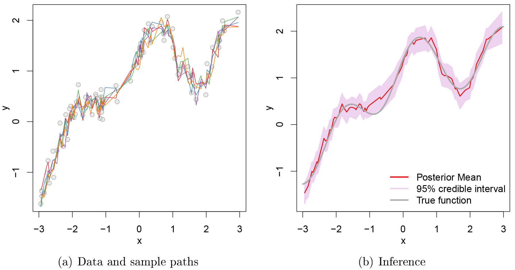
Now, in order to test the previous algorithm, we generate synthetic data according to Eq. (1) with $\sigma=0.2$ , $x_{i}\mathrel{\overset{\makebox[0.0pt]{\mbox{\@setsize{\tiny}{6pt}{\vpt}{\@vpt% }iid}}}{\sim}}\textsf{U}(-3,3)$ , for $i=1,\ldots,100$ , and the true regression function $f(x)=0.3+0.4x+0.5\sin(2.7x)+\frac{1.1}{1+x^{2}}$ (this example is included in a technical report by Radford Neal, which is available on-line from http://www.cs.toronto.edu/∼radford/mc-gp.abstract.html). Panel (a) in Fig. 1 shows the simulated dataset. Here, we adopt an empirical Bayes approach by setting $a_{\mu}=\bar{y}$ , $a_{\sigma}=a_{\tau}=2$ , $b_{\mu}=b_{\sigma}=b_{\tau}=s^{2}_{y}/3$ , since marginally $\textsf{E}(y_{i})=a_{\mu}=\bar{y}$ and $\textsf{Var}(y_{i})=b_{\mu}+b_{\sigma}+b_{\tau}=s^{2}_{y}$ ; and also, $a_{\phi}=0.1$ and $b_{\phi}=10$ , which let $\phi$ vary across a wide range of values. Thus, we fit the model with $\alpha=1$ and run the algorithm choosing $\delta$ (step 5.) carefully to produce a reasonable average mixing rate between 30% and 50%.

Table 1

Posterior summaries for $\sigma^{2}$ , $\mu$ , $\tau^{2}$ , and $\phi$

Parameter	Mean	SD	2.5%	50%	97.5%
$\sigma^{2}$	0.0334	0.0063	0.0228	0.0327	0.0476
$\mu$	0.6117	0.3932	$-$ 0.1654	0.6144	1.3862
$\tau^{2}$	0.8075	0.4035	0.3303	0.7009	1.8700
$\phi$	0.3590	0.1740	0.1200	0.3296	0.7710

Fig. 1.

Data along with five sample paths chosen at random from the posterior distribution of $\bm{\theta}$ , and posterior inference on $f(\cdot)$ .

The results presented below are based on $B=25000$ samples from the posterior distribution $p(\mathbf{\Upsilon}\mid\bm{y})$ obtained after thinning the original chain every 10 observations and a burn-in period of 5000 iterations. Chains mixed reasonably well and effective sample sizes for $\bm{\theta}$ range from 22921 to 26436. Panel (a) in Fig. 1 shows five sample paths chosen at random from the posterior distribution of $\bm{\theta}$ . We see how these paths fit very well to the data. On the other hand, Table 1 presents summaries the posterior distribution of $\sigma^{2}$ , $\mu$ , $\tau^{2}$ , and $\phi$ . Note that the 95% quantile-based credible interval for $\sigma^{2}$ includes the true value (0.04). Finally, Panel (b) in Fig. 1 shows the posterior mean along with 95% credible intervals for $f(\cdot)$ . Almost the entire true function falls within the credible bands, which shows that the model specification as well as the prior elicitation was suitable in this case.

3. Dynamic linear modelling

Figure 2 shows the detrended zero-centered weekly change series $y_{1},\ldots,y_{T}$ associated with the U.S. 3-year Treasury Constant Maturity Interest Rate from March 18, 1988 to September 10, 1999. We have $T=600$ equally spaced measurements in total. This series does not exhibit additional trends and seems to be stationary (which is confirmed below), so we do not differentiate the data again.

3.1 Autoregressive model

As a naive analysis of the series, we consider a model of the form

$\displaystyle y_{t}=\phi_{1}y_{t-1}+\ldots+\phi_{p}y_{t-p}+\epsilon_{t},\quad% \epsilon_{t}\mid v\mathrel{\overset{\makebox[0.0pt]{\mbox{\@setsize{\tiny}{6pt% }{\vpt}{\@vpt}iid}}}{\sim}}\textsf{N}(0,\upsilon),$ (2)

which corresponds to an autoregressive model of order $p$ , $\textsf{AR}(p)$ . We fit this model to the data using a reference prior distribution of the form $p(\bm{\phi},\upsilon)\propto 1/\upsilon$ , with $\bm{\phi}=(\phi_{1},\ldots,\phi_{p})$ , and the conditional likelihood

$\displaystyle p(\bm{y}\mid y_{1},\ldots,y_{p},\bm{\phi},\upsilon)=\prod_{t=p+1% }^{T}\textsf{N}(y_{t}\mid\mathbf{f}_{t}^{\textsf{T}}\bm{\phi},\upsilon)=% \textsf{N}_{T-p}(\bm{y}\mid\mathbf{F}^{\textsf{T}}\bm{\phi},\upsilon\mathbf{I})$ (3)

where $\bm{y}=(y_{p+1},\ldots,y_{T})$ since the first $p$ observations are considered as initial values, $\mathbf{f}_{t}=(y_{t-1},\ldots,y_{t-p})$ for $t=p+1,\ldots,T$ , and $\mathbf{F}=[\mathbf{f}_{p+1},\ldots,\mathbf{f}_{T}]$ . This formulation corresponds to a regular linear model setting, and therefore, we can apply standard theory (Prado & West, 2010, pp. 19–22).

Combining the likelihood Eq. (3) with the prior distribution $p(\bm{\phi},\upsilon)$ , we can easily obtain samples from the posterior distribution $p(\bm{\phi},\upsilon\mid\bm{y})$ using direct sampling as follows: first, sample $\upsilon$ from $\textsf{IG}((n-p)/2,(n-p)\hat{\upsilon}^{2}/2)$ , and then, for each $\upsilon$ in the previous step sample $\bm{\phi}$ from a $\textsf{N}_{p}(\hat{\bm{\phi}}_{\text{mle}},\upsilon(\mathbf{F}\mathbf{F}^{% \textsf{T}})^{-1})$ . Using $p=3$ , it follows that $n=T-p=597$ , $(n-p)\hat{\upsilon}^{2}=7.6759$ is the residual sum of squares, which in turn leads to $\hat{v}_{\text{mle}}=0.0128$ the MLE of $v$ , and $\hat{\bm{\phi}}_{\text{mle}}=(\mathbf{F}\mathbf{F}^{\textsf{T}})^{-1}\mathbf{F% }\bm{y}=(0.2283,0.0018,0.1146)$ is the MLE of $\bm{\phi}$ . Posterior summaries of 25000 samples from $p(\bm{\phi},\upsilon\mid\bm{y})$ are provided in Table 2. We see that the posterior parameter estimates are very similar to their MLE counterpart.

Table 2

Posterior summaries for $\bm{\phi}$ and $\upsilon$

Parameter	Mean	SD	2.5%	50%	97.5%
$\phi_{1}$	0.2267	0.0407	0.1462	0.2267	0.3066
$\phi_{2}$	0.0063	0.0420	$-$ 0.0753	0.0058	0.0896
$\phi_{3}$	0.1132	0.0408	0.0334	0.1132	0.1936
$\upsilon$	0.0130	0.0007	0.0116	0.0129	0.0145

Fig. 2.

Detrended zero-centered weekly change series of the U.S. 3-year Treasury Constant Maturity Interest Rate from March 18, 1988 to September 10, 1999.

3.2 Dynamic linear model

Now, going forward in the analysis, we consider a popular model given in (Tsay, 2010, p. 632) for detecting outliers:

$\displaystyle y_{t}=\gamma_{t}\alpha_{t}+x_{t}+\epsilon_{t},\quad\gamma_{t}% \mathrel{\overset{\makebox[0.0pt]{\mbox{\@setsize{\tiny}{6pt}{\vpt}{\@vpt}iid}% }}{\sim}}\textsf{Ber}(0.2),\quad\alpha_{t}\mathrel{\overset{\makebox[0.0pt]{% \mbox{\@setsize{\tiny}{6pt}{\vpt}{\@vpt}iid}}}{\sim}}\textsf{N}(0,0.1),\quad% \epsilon_{t}\mathrel{\overset{\makebox[0.0pt]{\mbox{\@setsize{\tiny}{6pt}{\vpt% }{\@vpt}iid}}}{\sim}}\textsf{N}(0,0.01),$ $\displaystyle x_{t}=\phi_{1}x_{t-1}+\ldots+\phi_{p}x_{t-p}+\eta_{t},\quad\eta_% {t}\mid\omega\mathrel{\overset{\makebox[0.0pt]{\mbox{\@setsize{\tiny}{6pt}{% \vpt}{\@vpt}iid}}}{\sim}}\textsf{N}(0,\omega).$ (4)

Under this formulation, $\gamma_{t}$ denotes the presence or absence of an additive outlier at time $t$ , and $\alpha_{t}$ its corresponding magnitude when present. Thus, additive outliers are allowed to occur at every time point with a probability equal to 0.2 (further details about the prior elicitation can be found in Tsay, 2010, p. 636). Furthermore, $x_{t}$ defines an autoregressive process with order $p$ . Then, we have $3T+p+1$ model parameters, namely, $\bm{\gamma}=(\gamma_{1},\ldots,\gamma_{T})$ , $\bm{\alpha}=(\alpha_{1},\ldots,\alpha_{T})$ , $\bm{x}=(x_{1},\ldots,x_{T})$ , $\bm{\phi}=(\phi_{1},\ldots,\phi_{p})$ , and $\omega$ . Also, we also assume the conjugate priors $\phi_{j}\mathrel{\overset{\makebox[0.0pt]{\mbox{\@setsize{\tiny}{6pt}{\vpt}{% \@vpt}iid}}}{\sim}}\textsf{N}(a_{\phi},b_{\phi})$ , for $j=1,\ldots,p$ , and $\omega\sim\textsf{IG}(a_{\omega},b_{\omega})$ .

Note that Eq. (3.2) is a non-Gaussian dynamic linear model (DLM). However, conditional on the outlier indicators $\gamma_{t}$ , this model can be written as a standard DLM. For instance, with $p=3$ the model aquires the form:

$\displaystyle y_{t}=\mathbf{F}^{\textsf{T}}\bm{\theta}_{t}+\nu_{t},\quad\nu_{t% }\mid V_{t}\mathrel{\overset{\makebox[0.0pt]{\mbox{\@setsize{\tiny}{6pt}{\vpt}% {\@vpt}ind}}}{\sim}}\textsf{N}(0,V_{t}),$ $\displaystyle\bm{\theta}_{t}=\mathbf{G}\bm{\theta}_{t-1}+\bm{\omega}_{t},\quad% \bm{\omega}_{t}\mid\mathbf{W}_{t}\mathrel{\overset{\makebox[0.0pt]{\mbox{% \@setsize{\tiny}{6pt}{\vpt}{\@vpt}ind}}}{\sim}}\textsf{N}_{p}(\bm{0},\mathbf{W% }_{t}),$ (5)

with

$\displaystyle\mathbf{F}=(1,0,0),\quad\bm{\theta}_{t}=(x_{t},x_{t-1},x_{t-2}),% \quad V_{t}=v_{\gamma_{t}}=\left\{\begin{array}[]{ll}0.01,&\hbox{$\gamma_{t}=0% $;}\\ 0.11,&\hbox{$\gamma_{t}=1$,}\end{array}\right.$

and

$\displaystyle\mathbf{G}=\begin{pmatrix}\phi_{1}&\phi_{2}&\phi_{3}\\ 1&0&0\\ 0&1&0\\ \end{pmatrix},\quad\bm{\omega}_{t}=(\eta_{t},0,0),\quad\mathbf{W}_{t}=\mathbf{% W}=\begin{pmatrix}\omega&0&0\\ 0&0&0\\ 0&0&0\\ \end{pmatrix}.$

We use the previous fact to develop the second step of the MCMC algorithm described below. There, we implement a forward filtering backward sampling algorithm (Prado & West, 2010, p. 137) to get samples from $p(\bm{\theta}_{1:T}\mid\bm{\gamma},\bm{\phi},\omega)$ , which automatically allow us to draw samples from $p(\bm{x}\mid\bm{\gamma},\bm{\phi},\omega)$ .

Now, we describe the general form of the MCMC to obtain samples from the posterior distribution

$\displaystyle p(\mathbf{\Upsilon}\mid\bm{y})\propto p(\bm{y}\mid\bm{\gamma},% \bm{\alpha},\bm{x})p(\bm{x}\mid\bm{\phi},w)p(\bm{\gamma})p(\bm{\alpha})p(\bm{% \phi})p(w),$

where $\mathbf{\Upsilon}=(\bm{\gamma},\bm{\alpha},\bm{x},\bm{\phi},\omega)$ and $\bm{y}=(y_{1},\ldots,y_{T})$ . Full conditional distributions are derived looking at the dependencies in $p(\mathbf{\Upsilon}\mid\bm{y})$ . Let $\mathbf{\Upsilon}^{(b)}$ be the vector of model parameters at iteration $b$ of the algorithm, for $b=1,\ldots,B$ . Given a starting point $\mathbf{\Upsilon}^{(0)}$ , we consider a Gibbs sampler (with a FFBS step) updating $\mathbf{\Upsilon}^{(b-1)}$ to $\mathbf{\Upsilon}^{(b)}$ until convergence as follows:

Sample $\alpha_{t}\mid\theta_{t,1},\gamma_{t},y_{t}\sim\textsf{N}(m_{t},V_{t})$ , for $t=1,\ldots,T$ , with

$\displaystyle V_{t}=\frac{1}{10(10\gamma_{t}+1)}\quad\text{and}\quad m_{t}=100% V_{t}\gamma_{t}(y_{t}-\theta_{t,1}).$

Sample $\gamma_{t}\mid\theta_{t,1},y_{t}\sim\textsf{Ber}(p_{t})$ , for $t=1,\ldots,T$ , with

$\displaystyle\frac{p_{t}}{1-p_{t}}=\frac{1}{4\sqrt{11}}\exp\left\{-{\textstyle% \frac{1}{2}}(y_{t}-\theta_{t,1})^{2}(1/0.11-1/0.01)\right\}.$

Sample $\bm{\phi}\mid\bm{\theta}_{1:T},\omega\sim\textsf{N}_{p}(\mathbf{m}_{\phi},% \mathbf{V}_{\bm{\phi}})$ , with

$\displaystyle\mathbf{V}_{\bm{\phi}}=\left(b_{\phi}^{-1}\mathbf{I}+\frac{1}{% \omega}\sum_{t=1}^{T}\bm{\theta}_{t-1}\bm{\theta}_{t-1}^{\textsf{T}}\right)^{-% 1}\quad\text{and}\quad\mathbf{m}_{\phi}=\mathbf{V}_{\bm{\phi}}\left(a_{\phi}b_% {\phi}^{-1}\mathbf{1}+\frac{1}{\omega}\sum_{t=1}^{T}\theta_{t,1}\bm{\theta}_{t% -1}\right).$

Sample $\omega\mid\bm{\theta}_{1:T},\bm{\phi}\sim\textsf{IG}(A_{\omega},B_{\omega})$ , with

$\displaystyle A_{\omega}=a_{\omega}+\frac{T}{2}\quad\text{and}\quad B_{\omega}% =b_{\omega}+\frac{1}{2}\sum_{t=1}^{T}(\theta_{t,1}-\bm{\phi}^{\textsf{T}}\bm{% \theta}_{t})^{2}.$

Sample $\bm{\theta}_{t}$ , for $t=1,\ldots,T$ , using a FFBS step. Here we use standard DLM notation, in particular that corresponding to the Kalman filter (West & Harrison, 1999, Theorem 4.1, pp. 103–105):

Use the filter equations to compute $\mathbf{a}_{t}$ , $\mathbf{R}_{t}$ , $\mathbf{m}_{t}$ , and $\mathbf{C}_{t}$ , for $t=1,\ldots,T$ :

$\displaystyle\mathbf{a}_{t}=\mathbf{G}_{t}\mathbf{m}_{t-1},\mathbf{R}_{t}=% \mathbf{G}_{t}\mathbf{C}_{t-1}\mathbf{G}_{t}^{\textsf{T}}+\mathbf{W}_{t},% \mathbf{m}_{t}=\mathbf{a}_{t}+\mathbf{A}_{t}e_{t},\mathbf{C}_{t}=\mathbf{R}_{t% }-Q_{t}\mathbf{A}_{t}\mathbf{A}_{t}^{\textsf{T}},$

with $e_{t}=y_{t}-f_{t}$ , $f_{t}=\mathbf{F}_{t}^{\textsf{T}}\mathbf{a}_{t}$ , and $Q_{t}=\mathbf{F}_{t}^{\textsf{T}}\mathbf{R}_{t}\mathbf{F}_{t}+V_{t}$ .

At time $t=T$ , sample $\bm{\theta}_{T}\sim\textsf{N}_{p}(\mathbf{m}_{T},\mathbf{C}_{T})$ .

For $t=(T-1),\ldots,0$ , sample $\bm{\theta}_{t}\sim\textsf{N}(\mathbf{m}_{t}^{*},\mathbf{C}_{t}^{*})$ , where

$\displaystyle\mathbf{m}_{t}^{*}=\mathbf{m}_{t}+\mathbf{B}_{t}(\bm{\theta}_{t+1% }-\mathbf{a}_{t+1})\quad\text{and}\quad\mathbf{C}_{t}^{*}=\mathbf{C}_{t}-% \mathbf{B}_{t}\mathbf{R}_{t+1}\mathbf{B}_{t}^{\textsf{T}},$

with $\mathbf{B}_{t}=\mathbf{C}_{t}\mathbf{G}_{t+1}^{\textsf{T}}\mathbf{R}_{t+1}^{-1}$ .

Now, we implement the MCMC provided above. To do so, we need to choose appropriate values for $a_{\phi}$ , $b_{\phi}$ , $a_{\omega}$ , and $b_{\omega}$ . First, $a_{\phi}=0$ and $b_{\phi}=0.25$ are reasonable values in accordance with our introductory analysis of the series using a standard autoregressive model. On the other hand, we weakly concentrate the prior distribution of $\omega$ around $\hat{\upsilon}_{\text{mle}}=0.0128$ from our introductory analysis, by setting $a_{\omega}=2$ and $b_{\omega}=\hat{\upsilon}_{\text{mle}}$ , which leads to $\textsf{E}(\omega)=\hat{\upsilon}_{\text{mle}}$ with infinite variance. The results presented below are based on $B=25000$ samples from the posterior distribution $p(\mathbf{\Upsilon}\mid\bm{y})$ obtained after a burn-in period of 5000 iterations. Chains mixed very well and there is no sign of lack of convergence. Effective sample sizes range from 398.7 to 29019.3.

Table 3

Posterior summaries for $\bm{\phi}$ and $\omega$

Parameter	Mean	SD	2.5%	50%	97.5%
$\phi_{1}$	0.4692	0.1605	0.1618	0.4665	0.7904
$\phi_{2}$	0.1341	0.1932	$-$ 0.2694	0.1492	0.4727
$\phi_{3}$	0.1296	0.1367	$-$ 0.1495	0.1309	0.4029
$\omega$	0.0017	0.0004	0.0010	0.0016	0.0026

Fig. 3.

(a) Posterior probability that an observation is an outlier (lines correspond to 0.5 and 0.8, which serve as probability thresholds). (b) Posterior mean of an outlier size.

Table 3 displays summaries for the posterior distribution of $\bm{\phi}$ and $\omega$ . Estimates for $\phi_{3}$ and $\omega$ are consistent with those obtained in Table 2 using a standard autoregressive model. However, estimates for $\phi_{1}$ and $\phi_{2}$ are utterly different. Such a difference is expected since the autoregressive model does not consider additive outliers, and as a consequence, is not able to characterize fundamental features of the series such as its mean evolution. On the other hand, Fig. 3 shows the posterior probability that an observation is an outlier $\textsf{Pr}(\gamma_{t}=1\mid\bm{y})$ along with the corresponding posterior mean of an outlier size $\textsf{E}(\alpha_{t}\mid\bm{y})$ , for $t=1,\ldots,T$ . We identify 18 observations such that $\textsf{Pr}(\gamma_{t}=1\mid\bm{y})>0.5$ , seven of which are greater than 0.8, namely, observation at weeks 65, 74, 201, 323, 415, 418, and 513. Tsay (2010, p. 564) also classifies these points as outliers (employing an approach with mild differences from the one described here) and highlight observations at times $t=323$ (May 20, 1994) and $t=201$ (January 17, 1992). At the former, there was a 0.6% drop in the weekly interest rate, while at the later, there was a jump of about 0.35%. Finally, Fig. 4 displays the estimated autoregressive process as well as the fitted values along with the original data. We see that the model captures reasonably well the “volatility” of the series.

Fig. 4.

(a) Posterior inference on the autoregressive process. (b) Data (gray) and fitted values (red).

4. Areal unit space-time modelling

We consider an ecological study in which a spatiotemporal model for areal unit data is considered for modelling a set of binary observations $y_{i,t}=y_{t}(\bm{s}_{i})$ , for $i=1,\ldots,I$ and $t=1,\ldots,T$ , in a discrete time period over a fixed lattice $\bm{s}_{1},\ldots,\bm{s}_{I}$ . Here, we consider the Google flu data corresponding to the first 12 weeks of 2013 for the contiguous continental states in the United States (Alaska and Hawaii are omitted from the analysis). Thus, we record a binary variable $y_{i,t}$ that is equal to 1 if the Google flue index for state $i$ during week $t$ is greater than 7500 cases, and 0 otherwise.

We have that the observations $y_{i,t}$ are Bernoulli distributed with probability of success $\pi_{i,t}$ , i.e., $y_{i,t}\mid\pi_{i,t}\sim\textsf{Ber}(\pi_{i,t})$ . Here, we consider the following areal hierarchical generalized linear model (Banerjee et al., 2014, Sec. 6.4) including a temporal component:

$\displaystyle y_{i,t}\mid\omega_{i,t}=\left\{\begin{array}[]{ll}1,&\text{if }% \omega_{it}>0;\\ 0,&\text{if }\omega_{it}\leqslant 0,\\ \end{array}\right.$ $\displaystyle\omega_{i,t}\mid\bm{\beta},\bm{\gamma},\xi,\theta_{i,t},\phi_{i,t% },\kappa_{t}\mathrel{\overset{\makebox[0.0pt]{\mbox{\@setsize{\tiny}{6pt}{\vpt% }{\@vpt}ind}}}{\sim}}\textsf{N}(\bm{x}_{i}^{\textsf{T}}\bm{\beta}+\bm{z}_{i}^{% \textsf{T}}\bm{\gamma}+\xi t+\theta_{i,t}+\phi_{i,t},1/\kappa_{t}),$ (6)

with a hierarchical prior distribution of the form

$\displaystyle\begin{array}[]{lll}\beta_{k}\mathrel{\overset{\makebox[0.0pt]{% \mbox{\@setsize{\tiny}{6pt}{\vpt}{\@vpt}iid}}}{\sim}}\textsf{N}(0,\sigma^{2}_{% 0}),&\gamma_{\ell}\mathrel{\overset{\makebox[0.0pt]{\mbox{\@setsize{\tiny}{6pt% }{\vpt}{\@vpt}iid}}}{\sim}}\textsf{CAR}(1/\sigma^{2}_{0}),&\xi\sim\textsf{N}(0% ,\sigma^{2}_{0}),\\ \theta_{i,t}\mid\tau_{t}\mathrel{\overset{\makebox[0.0pt]{\mbox{\@setsize{% \tiny}{6pt}{\vpt}{\@vpt}ind}}}{\sim}}\textsf{N}(0,1/\tau_{t}),&\phi_{i,t}\mid% \lambda_{t}\mathrel{\overset{\makebox[0.0pt]{\mbox{\@setsize{\tiny}{6pt}{\vpt}% {\@vpt}ind}}}{\sim}}\textsf{CAR}(\lambda_{t}),&\kappa_{t}\mathrel{\overset{% \makebox[0.0pt]{\mbox{\@setsize{\tiny}{6pt}{\vpt}{\@vpt}iid}}}{\sim}}\textsf{G% }(\nu_{0}/2,\nu_{0}/2),\\ \tau_{t}\mathrel{\overset{\makebox[0.0pt]{\mbox{\@setsize{\tiny}{6pt}{\vpt}{% \@vpt}iid}}}{\sim}}\textsf{G}(a_{\tau},b_{\tau}),&\lambda_{t}\mathrel{\overset% {\makebox[0.0pt]{\mbox{\@setsize{\tiny}{6pt}{\vpt}{\@vpt}iid}}}{\sim}}\textsf{% G}(a_{\lambda},b_{\lambda}),\\ \end{array}$ (7)

for $k=1\ldots,K$ , $\ell=1,\ldots,L$ , where $\nu_{0}$ is a fixed positive integer, $\sigma^{2}_{0},a_{\tau},b_{\tau},a_{\lambda},b_{\lambda}$ are fixed positive real numbers, and $\bm{\beta}=(\beta_{1},\ldots,\beta_{K})$ , $\bm{x}_{i}=\bm{x}(\bm{s}_{i})=(x_{1}(\bm{s}_{i}),\ldots,x_{K}(\bm{s}_{i}))$ are location-specific fixed effects, $\bm{\gamma}=(\gamma_{1},\ldots,\gamma_{L})$ , and $\bm{z}_{i}=\bm{z}_{t}(\bm{s}_{i})=(z_{1}(\bm{s}_{i}),\ldots,z_{L}(\bm{s}_{i}))$ are location-specific random effects. Thus, $L$ denotes the number of random effects associated with the locations. Finally, notice that in Eq. (4) we have included the auxiliary variables $\omega_{i,t}$ in order to ease computation and performance Chib (1995).

The link function $g(\cdot)$ relating the $\pi_{i,t}$ and the linear predictor is based in a Student-t distribution with $\nu_{0}$ degrees of freedom, which is particularly useful to detect rare events (those with small $\pi_{i,t}$ ). Since $\omega_{i,t}=\eta_{i,t}+\epsilon_{i,t}$ with $\eta_{i,t}=\bm{x}_{i}^{\textsf{T}}\bm{\beta}+\bm{z}_{i}^{\textsf{T}}\bm{\gamma% }+\xi t+\theta_{i,t}+\phi_{i,t}$ , $\epsilon_{i,t}\sim\textsf{N}(0,1/\kappa_{t})$ and $\kappa_{t}\sim\textsf{G}(\nu_{0}/2,\nu_{0}/2)$ , then the marginal distribution of $\epsilon_{i,t}$ (and therefore $\omega_{it}$ ) is Student-t with $\nu_{0}$ degrees of freedom. Thus, due to the symmetry of the t distribution, we have that $\textsf{Pr}\left(y_{i,t}=1\mid\omega_{i,t}\right)=\textsf{Pr}\left(\epsilon_{% it}\leqslant\eta_{i,t}\right)$ , and therefore, $\pi_{i,t}=F_{\nu_{0}}(\eta_{i,t})$ , where $F_{\nu_{0}}$ is the cumulative distribution functions of a random variable following a t distribution with $\nu_{0}$ degrees of freedom, which means that the link function is $g=F_{\nu_{0}}$ .

Note that the main effects for non-spatiotemporal covariates have a standard linear regression structure $\bm{x}_{i}^{\textsf{T}}\bm{\beta}$ , with a weakly informative prior for $\bm{\beta}$ (Gelman et al., 2014, p. 55). Also, the main effects for space covariates have a standard linear regression structure $\bm{z}_{i}^{\textsf{T}}\bm{\gamma}$ , following an improper conditionally autoregressive (CAR) model for $\bm{\gamma}$ (Banerjee et al., 2014, p. 81). Furthermore, the main effects for time are included in the linear predictor through $\delta_{t}=\xi t$ , with a weakly informative prior for $\xi$ . Lastly, the main effects for spatiotemporal interactions $\theta_{i,t}+\phi_{i,t}$ have two components. On the one hand, $\theta_{i,t}$ captures region-wide heterogeneity (unstructured variation) by means of $\textsf{N}(0,1/\tau_{t})$ , where $\tau_{t}$ is a precision parameter controlling the magnitude of $\theta_{i,t}$ . And on the other, $\phi_{i,t}$ captures regional clustering (spatially structured variability) via $\textsf{CAR}(\lambda_{t})$ , where $\lambda_{t}$ is a precision parameter as before.

CAR models are very convenient computationally, since the method for exploring the posterior distribution is in itself a conditional algorithm, the Gibbs sampler, which also eliminates the need for matrix inversion. However, CAR models have two main theoretical and computational challenges, namely, model impropriety and precision parameter selection. Banerjee et al. (2014, p. 155) recommend to ignore impropriety and work with the intrinsic CAR specification, since we are using it just as a prior distribution and not to model the data directly. Even though this is the usual approach it requires some care: This improper CAR prior is a pairwise difference prior that is identified only up to an additive constant. Thus, in order to identify an intercept term (say $\beta_{1}$ ), we must add the constraint $\sum_{i=1}^{I}\phi_{i,t}=0$ (this constrain is imposed numerically during computation). Moreover, $\tau_{t}$ and $\lambda_{t}$ cannot be chosen arbitrarily large, since $\theta_{i,t}$ and $\phi_{i,t}$ would become unidentifiable. After all, we have only a single $y_{i,t}$ in order to estimate two random effects for each $i$ and each $t$ . To make the prior specification $\tau_{t}\sim\textsf{G}(a_{\tau},b_{\tau})$ and $\lambda_{t}\sim\textsf{G}(a_{\lambda},b_{\lambda})$ sensible, Banerjee et al. (2014, p. 156) recommend a prior specification that leads to

$\displaystyle\textsf{SD}(\theta_{i,t})=\frac{1}{\sqrt{\tau_{t}}}\approx\frac{1% }{0.7\sqrt{\bar{m}\lambda_{t}}}\approx\textsf{SD}(\phi_{i,t}),$ (8)

where $\bar{m}$ is the average number of neighbors.

Fig. 5.

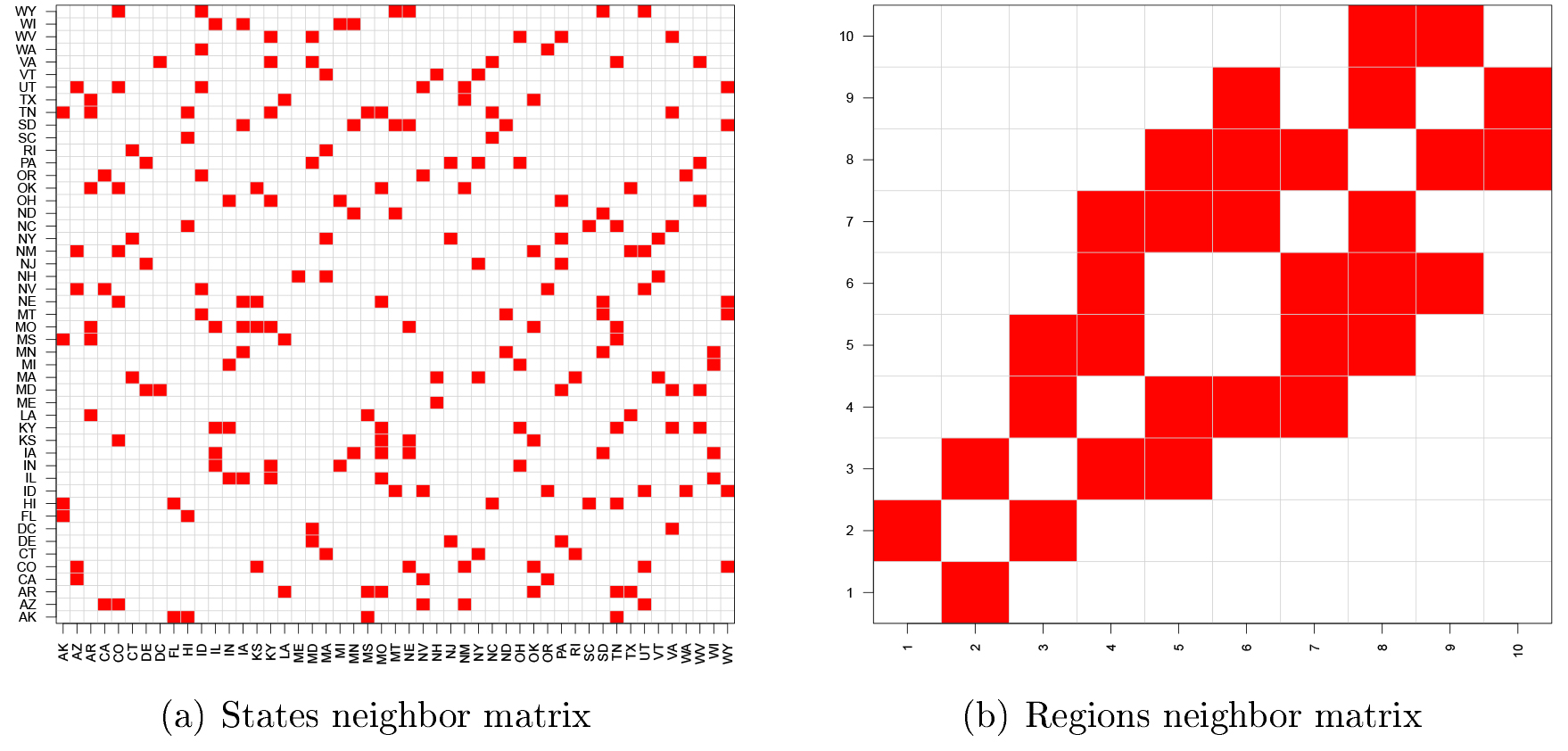
States and regions neighbors used to specify precision matrices. Red boxes denote neighbor elements.

Define $\bm{y}=(y_{1,1},\ldots,y_{I,T})$ , $\bm{\omega}=(\omega_{1,1},\ldots,\omega_{I,T})$ , $\bm{\theta}=(\theta_{1,1},\ldots,\theta_{I,T})$ , $\bm{\phi}=(\phi_{1,1},\ldots,\phi_{I,T})$ , $\bm{\kappa}=(\kappa_{1},\ldots,\kappa_{T})$ , $\bm{\tau}=(\tau_{1},\ldots,\tau_{T})$ , $\bm{\lambda}=(\lambda_{1},\ldots,\lambda_{T})$ , and also, $\mathbf{\Upsilon}=(\bm{\omega},\bm{\theta},\bm{\phi},\bm{\beta},\bm{\gamma},\xi)$ . Parameter estimates can be obtained from the posterior distribution

$\displaystyle p(\mathbf{\Upsilon}\mid\bm{y})\propto p(\bm{y}\mid\bm{\omega})p(% \bm{\omega}\mid\bm{\theta},\bm{\phi},\bm{\beta},\bm{\gamma},\xi,\bm{\kappa})p(% \bm{\theta}\mid\bm{\tau})p(\bm{\phi}\mid\bm{\lambda})p(\bm{\beta})p(\bm{\gamma% })p(\xi)p(\bm{\kappa})p(\bm{\tau})p(\bm{\lambda}),$

where according to Eqs (4) and (7),

$\displaystyle p(\bm{\omega}\mid\bm{\beta},\bm{\gamma},\bm{\theta},\xi,\bm{\phi% },\bm{\kappa})=\prod_{i=1}^{I}\prod_{t=1}^{T}\textsf{N}(\omega_{i,t}\mid\bm{x}% _{i}^{\textsf{T}}\bm{\beta}+\bm{z}_{i}^{\textsf{T}}\bm{\gamma}+\xi t+\theta_{i% ,t}+\phi_{i,t},1/\kappa_{t}),$ $\displaystyle p(\bm{\theta}\mid\bm{\tau})=\textsf{N}_{IT}(\bm{\theta}\mid\bm{0% },\textsf{diag}[(1/\tau_{1})\mathbf{I}_{I},\ldots,(1/\tau_{T})\mathbf{I}_{I}]),$ $\displaystyle p(\bm{\phi}\mid\bm{\lambda})=\textsf{CAR}(\bm{\phi}\mid\textsf{% diag}[\lambda_{1}\mathbf{W},\ldots,\lambda_{T}\mathbf{W}]),$ $\displaystyle p(\bm{\beta})p(\bm{\gamma})p(\xi)p(\bm{\kappa})p(\bm{\tau})p(\bm% {\lambda})=p(\xi)\times\prod_{k=1}^{K}p(\beta_{k})\times\prod_{\ell=1}^{L}p(% \gamma_{\ell})\times\prod_{t=1}^{T}p(\kappa_{t})p(\tau_{t})p(\lambda_{t}),$

with $p(\xi),p(\beta_{k}),p(\gamma_{\ell}),p(\kappa_{t}),p(\tau_{t}),p(\lambda_{t})$ specified as in Eq. (7), and $\mathbf{W}=[W_{i,j}]$ is a square matrix of size $I\times I$ such that

$\displaystyle W_{i,j}=\left\{\begin{array}[]{ll}m_{i},&{i=j;}\\ -1,&{i\sim j;}\\ 0,&\text{otherwise},\\ \end{array}\right.$

where $m_{i}$ is the number of neighbors of $\bm{s}_{i}$ (see Fig. 5), and $i\sim j$ means that units $i$ and $j$ are neighbors. Full conditional distributions are derived looking at the dependencies in $p(\mathbf{\Upsilon}\mid\bm{y})$ . Let $\mathbf{\Upsilon}^{(b)}$ be the vector of model parameters at iteration $b$ of the algorithm, for $b=1,\ldots,B$ . Given a starting point $\mathbf{\Upsilon}^{(0)}$ , we consider a Gibbs sampler (with a step with a numerical constraint) updating $\mathbf{\Upsilon}^{(b-1)}$ to $\mathbf{\Upsilon}^{(b)}$ until convergence as follows:

Sample

$\displaystyle\omega_{i,t}\mid\text{rest}\sim\left\{\begin{array}[]{ll}\textsf{% TN}_{(-\infty,0]}(\bm{x}_{i}^{\textsf{T}}\bm{\beta}+\bm{z}_{i}^{\textsf{T}}\bm% {\gamma}+\xi t+\theta_{i,t}+\phi_{i,t},1/\kappa_{t}),&y_{it}=0;\\ \textsf{TN}_{(0,+\infty)}(\bm{x}_{i}^{\textsf{T}}\bm{\beta}+\bm{z}_{i}^{% \textsf{T}}\bm{\gamma}+\xi t+\theta_{i,t}+\phi_{i,t},1/\kappa_{t}),&y_{it}=1,% \\ \end{array}\right.$

for $i=1,\ldots,I$ , $t=1,\ldots,T$ .

Sample

$\displaystyle\bm{\beta}\mid\text{rest}\sim\textsf{N}_{K}(\mathbf{V}_{\bm{\beta% }}\left[\mathbf{X}^{\textsf{T}}\mathbf{\Sigma}^{-1}_{\bm{\omega}}(\bm{w}-% \mathbf{Z}\bm{\gamma}-\bm{t}\xi-\bm{\theta}-\bm{\phi})\right],\mathbf{V}_{\bm{% \beta}})$

where $\mathbf{V}_{\bm{\beta}}=(\sigma_{0}^{-2}\mathbf{I}_{K}+\mathbf{X}^{\textsf{T}}% \mathbf{\Sigma}^{-1}_{\bm{\omega}}\mathbf{X})^{-1}$ , $\mathbf{\Sigma}^{-1}_{\bm{\omega}}=\text{diag}\left[\bm{1}_{I}\otimes\bm{% \kappa}\right]$ , $\bm{t}=\bm{1}_{I}\otimes[t_{1},\ldots,t_{T}]^{\textsf{T}}$ , $\mathbf{X}=[\mathbf{X}_{1}^{\textsf{T}},\ldots,\mathbf{X}_{I}^{\textsf{T}}]^{% \textsf{T}}$ , with $\mathbf{X}_{i}=\bm{1}_{T}\otimes\bm{x}_{i}^{\textsf{T}}$ for $i=1,\ldots,I$ , $\mathbf{Z}=[\mathbf{Z}_{1}^{\textsf{T}},\ldots,\mathbf{Z}_{I}^{\textsf{T}}]^{% \textsf{T}}$ , with $\mathbf{Z}_{i}=\bm{1}_{T}\otimes\bm{z}_{i}^{\textsf{T}}$ for $i=1,\ldots,I$ .

Sample

$\displaystyle\bm{\gamma}\mid\text{rest}\sim\textsf{N}_{L}\left(\mathbf{V}_{\bm% {\gamma}}\left[\mathbf{Z}^{\textsf{T}}\mathbf{\Sigma}^{-1}_{\bm{\omega}}(\bm{w% }-\mathbf{X}\bm{\beta}-\bm{t}\xi-\bm{\theta}-\bm{\phi})\right],\mathbf{V}_{\bm% {\gamma}}\right)$

where $\mathbf{V}_{\bm{\gamma}}=(\sigma_{0}^{-2}\mathbf{W}^{*}+\mathbf{Z}^{\textsf{T}% }\mathbf{\Sigma}^{-1}_{\bm{\omega}}\mathbf{Z})^{-1}$ and $\mathbf{W}^{*}$ is a precision matrix (covariance matrix inverse) of size $L\times L$ defined accordingly (see Fig. 5, panel b).

Sample

$\displaystyle\xi\mid\text{rest}\sim\textsf{N}\left(V_{\xi}\left[\bm{t}^{% \textsf{T}}\mathbf{\Sigma}^{-1}_{\bm{\omega}}(\bm{w}-\mathbf{X}\bm{\beta}-% \mathbf{Z}\bm{\gamma}-\bm{\theta}-\bm{\phi})\right],V_{\xi}\right)$

where $V_{\xi}=(\sigma_{0}^{-2}+\bm{t}^{\textsf{T}}\mathbf{\Sigma}^{-1}_{\bm{\omega}}% \bm{t})^{-1}$ .

Fig. 6.

Regional offices according to the U.S. Department of Health and Human Services.

Sample

$\displaystyle\bm{\theta}_{t}\mid\text{rest}\sim\textsf{N}_{I}\left(\mathbf{V}_% {t}\left[\kappa_{t}(\bm{\omega}_{t}-\mathbf{X}_{t}\bm{\beta}-\mathbf{Z}_{t}\bm% {\gamma}-\bm{t}_{t}\xi-\bm{\phi}_{t})\right],\mathbf{V}_{t}\right)$

where $\bm{\theta}_{t}=(\theta_{1t},\ldots,\theta_{It})$ , $\mathbf{V}_{t}=(\tau_{t}+\kappa_{t})^{-1}\mathbf{I}_{I}$ , $\bm{\omega}_{t}=(\omega_{1t},\ldots,\omega_{It})$ , $\mathbf{X}_{t}=[\bm{x}_{1},\ldots,\bm{x}_{I}]^{\textsf{T}}$ , $\mathbf{Z}_{t}=[\bm{z}_{1},\ldots,\bm{z}_{I}]^{\textsf{T}}$ , and $\bm{t}_{t}=t\bm{1}_{I}$ , for $t=1,\ldots,T$ .

Sample

$\displaystyle\bm{\phi}_{t}\mid\text{rest}\sim\textsf{N}_{I}\left(\mathbf{V}_{t% }\left[\kappa_{t}(\bm{\omega}_{t}-\mathbf{X}_{t}\bm{\beta}-\mathbf{Z}_{t}\bm{% \gamma}-\bm{t}_{t}\xi-\bm{\theta}_{t})\right],\mathbf{V}_{t}\right)$

where $\bm{\phi}_{t}=(\phi_{1t},\ldots,\phi_{It})$ and $\mathbf{V}_{t}=(\lambda_{t}\mathbf{W}+\kappa_{t}\mathbf{I}_{I})^{-1}$ , for $t=1,\ldots,T$ .

Center $\bm{\phi}_{t}$ around its own mean in order to impose the constrain $\sum_{i=1}^{I}\phi_{i,t}=0$ , for $t=1,\ldots,T$ .

Sample $\kappa_{t}\mid\text{rest}\sim\textsf{G}\left(({\nu_{0}+I})/2,\left({\nu_{0}+\|% \bm{w}_{t}-\mathbf{X}_{t}\bm{\beta}-\mathbf{Z}_{t}\bm{\gamma}-\bm{t}_{t}\xi-% \bm{\theta}_{t}-\bm{\phi}_{t}\|^{2}}\right)/2\right)$ , for $t=1,\ldots,T$ .

Sample $\tau_{t}\mid\text{rest}\sim\textsf{G}(a_{\tau}+{\textstyle\frac{I}{2}},b_{\tau% }+{\textstyle\frac{1}{2}}{\|\bm{\theta}_{t}\|^{2}})$ , for $t=1,\ldots,T$ .

10.

Sample $\lambda_{t}\mid\text{rest}\sim\textsf{G}(a_{\lambda}+{\textstyle\frac{1}{2}}{% \operatorname*{rank}(\mathbf{W})},b_{\lambda}+{\textstyle\frac{1}{2}}{\bm{\phi% }_{t}^{\textsf{T}}\mathbf{W}\bm{\phi}_{t}})$ , for $t=1,\ldots,T$ .

Now, we implement the model by considering the Google flu data corresponding to the first 12 weeks of 2013. Outbreaks of influenza are commonly observed during weeks 1 to 8 (Winter season). The proportion of states with Google flue index greater than 7500 cases goes down straight to zero after week 8. Then, we have an align dataset with $I=49$ states (subjects) and $T=12$ weeks (period times) that lead to 637 observations possibly correlated in time and space. Thus, we consider the linear predictor given by

$\displaystyle F_{\nu_{0}}^{-1}(\pi_{i,t})=\beta_{1}+\beta_{2}x_{i,1}+\beta_{3}% x_{i,2}+\gamma_{\ell}z_{i,\ell}+\xi t+\theta_{i,t}+\phi_{i,t}$ (9)

where $x_{i,1}$ and $x_{i,2}$ are the proportion of white population and the proportion of population over 65 years old, respectively, for state $i$ in 2013, according to Kaiser Family Foundation (http://kff.org/), and $z_{i,\ell}$ is an indicator variable pointing out if state $i$ belongs to region $\ell$ or not, according to according to the U.S. Department of Health and Human Services (HHS, http://www.hhs.gov/iea/regional/; see Fig. 6). Therefore, $\beta_{1}$ is the mean global effect, $\beta_{k}$ is the fixed effect of covariate $k$ , for $k=2,3$ , $\gamma_{\ell}$ is the fixed spacial effect of region $\ell$ , for $\ell=1,\ldots,10$ , $\xi$ is the fixed effect of time, and $\theta_{i,t}+\phi_{i,t}$ is the random spatiotemporal effect considering heterogeneity and clustering.

Fig. 7.

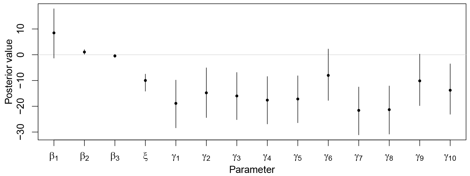
Posterior mean and 95% quantile-based credible intervals for $\bm{\beta}$ , $\xi$ , and $\bm{\gamma}$ .

Fig. 8.

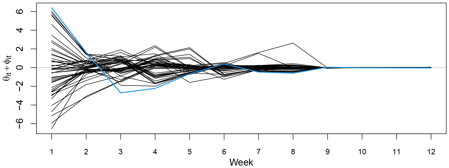
Posterior mean for the dynamic random effects $\theta_{i,t}+\phi_{i,t}$ . The blue line corresponds to Maine, which is the state with the highest proportion of white population in 2013.

We implement the MCMC algorithm given above drawing $B=25000$ samples from the posterior distribution $p(\mathbf{\Upsilon}\mid\bm{y})$ after thinning the original chain every 10 observations and a burn-in period of 5000 iterations. To do so, we weakly concentrate the prior distribution of $\beta_{k}$ , $\gamma_{\ell}$ , and $\xi$ around 0, and that of $\kappa_{t}$ , $\tau_{t}$ , and $\lambda_{t}$ around 1, by following the prior specification given in Eq. (8) with $\sigma^{2}_{0}=100$ , $\nu_{0}=a_{\tau}=b_{\tau}=a_{\lambda}=2$ , and $b_{\lambda}=(0.7^{2})\bar{m}b_{\tau}$ . Notice that $\nu_{0}$ is set equal to 2 because a $\textsf{t}_{2}$ distribution has an infinite variance. Trace and autocorrelation plots of the regression parameters show that the corresponding chains achieve convergence quickly. However, in some particular cases, there are signs of serious autocorrelation (in order to address this issue we thin the chain as specified).

Figure 7 summarizes the posterior distribution of $\bm{\beta}$ , $\xi$ , and $\bm{\gamma}$ . The proportion of the white population have a positive significant impact on the response, which leads to an increment in the probability that the state is above the threshold, whereas the global mean and the proportion of population over 65 do not. Even thought most deaths associated with influenza in industrialized countries occur among the elderly over 65 years of age, this covariate results not significant because it has little variation across the states ( $\textsf{CV}\doteq 11\%$ ) and the proportion of population over 65 in each state is just a small fraction of the whole state population (be aware of the “ecological fallacy”). In addition, such a finding makes sense because we are considering incidence as opposed to mortality. Furthermore, all the regions delimited by the HHS have a significant impact on the response, excepting regions 6 and 9 (see Fig. 6). This finding is reasonable since these regions are neighbors and are the smallest regions in terms of extension and population. In addition, it is not surprising that in general regions have a negative influence on the response since these regions independently address needs of communities and individuals through HHS programs and policies. Finally, the effect of time is also significant since it is well known that outbreaks of flue are highly correlated with seasons and we consider a time transition frame.

On the other hand, Fig. 8 displays the posterior mean for the sum of the heterogeneity and clustering random effects $\theta_{i,t}+\phi_{i,t}$ . As expected, these effects clearly go down toward 0 after week 8 due to the seasonal behavior of the response. Even though all the states reveal similar patterns, the model is also useful to identify subject-specific dynamic effects. For instance, consider the case of Maine (ME), which is the state with the highest proportion of white population in 2013.

5. Discussion

In this work we have offered four detailed case studies that use Bayesian modelling techniques in order to answer complex questions. At every instance, we have provided specifics about model formulation, prior elicitation, simulation-based algorithms computation, and posterior inference. We hope that the reader benefits from such effort and considers the Bayesian paradigm a natural way to solve data-driven problems.

From a frequentist point of view, an extra effort is needed in order to fit the kind of models that we consider in this work. On the one hand, for “random effects”, once we specify a stochastic dependence for a given parameter (this is quite natural under the Bayesian paradigm because all parameters are random quantities), its condition becomes unclear for carrying out frequentist inference: Are random effects parameters or not? On the other hand, from a Bayesian perspective, since both observations and parameters are random variables, dealing with missing and censored data as well as uncertainty quantification is straightforward, even more so since simulation-based approaches became widely available in the early 90s (Robert & Casella, 2011). Finally, it is noteworthy that frequentists deal directly (in an ad-hoc fashion) with hierarchical models by maximizing either marginal likelihoods or restricted maximum likelihoods Patterson and Thompson (1971), or treating random effects (or any other set of parameters) as missing data and estimate them using and EM algorithm (Dempster et al., 1977).

Even though the Bayesian approach to statistical inference is extremely beneficial, some challenges remain. The most challenging aspects of Bayesian statistical inference correspond to eliciting prior distributions and performing the prior-to-posterior updates in non-conjugate models.

The prior distribution is an integral part of the model and needs as much attention as the likelihood function. If the prior information is “bad”, then it could negatively affect the results (on the flip side, “good” prior information can substantially improve the quality of your results, particularly for small sample sizes). Also, the prior elicitation can be very complex when many hyperparameters need to be set (often associated to parametric families). Even after the introduction of more powerful computational tools based on simulations, the choice of prior distributions is often driven by a desire to facilitate computation.

Typically, the prior-to-posterior updates is a much more challenging problem than that encountered in classical statistical methods. Computation for frequentist methods requires that we compute maximums and derivatives. Computation for Bayesian methods usually requires that we compute integrals. This was a major obstacle for the practical adoption of Bayesian methods before cheap and powerful computers were widely available until the early 90s (see our discussion above). Finally, we recommend consider alternative inference methods in order to account for “big data”, which is currently an active research area in computational statistics (e.g., variational methods). See for example Ormerod and Wand (2010).

Lastly, we devote a few words in order to demystify the gap between frequentist and Bayesian thinking. After reviewing some advantages and challenges of the Bayesian paradigm, the reader should be aware that several links with the frequentist world remain. For instance, as part of the revision process, one of the referees pointed out the connection between the frequentist treatment of mixed effects models and empirical Bayes methods: The best linear unbiased prediction for random effects under the frequentist paradigm can also be obtain directly from empirical Bayes principles (e.g., Karunamuni, 2002). Other similarities are available, mostly under noninformative prior distributions and large sample sizes, but they will be discussed elsewhere.

Footnotes

Appendix

Notation and acronyms

The cardinality of a set $A$ is denoted by $|A|$ . If P is a logical proposition, then $\mathbf{1}\left\{\text{P}\right\}=1$ if P is true, and $\mathbf{1}\left\{\text{P}\right\}=0$ if P is false. $\lfloor x\rfloor$ denotes the floor of $x$ , whereas $[n]$ denotes the set of all integers from 1 to $n$ , i.e., $\{1,\ldots,n\}$ . The Gamma function is given by $\Gamma(x)=\int_{0}^{\infty}u^{x-1}e^{-u}\text{d}u$ .

Matrices and vectors with entries consisting of subscripted variables are denoted by a boldfaced version of the letter for that variable. For example, $\bm{x}=(x_{1},\ldots,x_{n})$ denotes an $n\times 1$ column vector with entries $x_{1},\ldots,x_{n}$ . We use $\bm{0}$ and $\bm{1}$ to denote the column vector with all entries equal to 0 and 1, respectively, and $\mathbf{I}$ to denote the identity matrix. A subindex in this context refers to the corresponding dimension; for instance, $\mathbf{I}_{K}$ denotes the $K\times K$ identity matrix. The transpose of a vector $\bm{x}$ is denoted by $\bm{x}^{T}$ ; analogously for matrices. Moreover, if $\mathbf{X}$ is a square matrix, we use $\textsf{tr}(\mathbf{X})$ to denote its trace and $\mathbf{X}^{-1}$ to denote its inverse. The norm of $\bm{x}$ , given by $\sqrt{\bm{x}^{T}\bm{x}}$ , is denoted by $\|\bm{x}\|$ .

The following list summarizes all the acronyms used in this manuscript. All the probability distributions can be found in Appendix A of (Gelman et al., 2014):

•

E: Expected value.

•

Var: Variance.

•

SD: Standard deviation.

•

CV: Coefficient of variation.

•

Pr: Probability.

•

Ber: Bernoulli distribution.

•

N: Normal distribution.

•

TN: Truncated normal distribution.

•

G: Gamma distribution.

•

IG: Inverse-gamma distribution.

•

U: Uniform distribution.

•

CAR: Conditionally autoregressive model.

•

GP: Gaussian process.

References

Banerjee

Carlin

, & Gelfand

(2014). Hierarchical modeling and analysis for spatial data. Crc Press.

Chib

(1995). Marginal likelihood from the gibbs output. Journal of the American Statistical Association, 90(432), 1313-1321.

Dempster

A.P.

Laird

N.M.

, & Rubin

D.B.

(1977). Maximum likelihood from incomplete data via the em algorithm. Journal of the Royal Statistical Society: Series B (Methodological), 39(1), 1-22.

Gelman

Carlin

Stern

, & Rubin

(2014). Bayesian data analysis, Vol. 2. Taylor & Francis.

Jackman

(2009). Bayesian analysis for the social sciences, Vo. 846. John Wiley & Sons.

Karunamuni

R.J.

(2002). An empirical bayes derivation of best linear unbiased predictors. International Journal of Mathematics and Mathematical Sciences, 31(12), 703-714.

Mü ller

Quintana

F.A.

Jara

, & Hanson

(2015). Bayesian nonparametric data analysis. Springer.

Ormerod

, & Wand

M.P.

(2010). Explaining variational approximations. The American Statistician, 64(2), 140-153.

Patterson

H.D.

, & Thompson

(1971). Recovery of inter-block information when block sizes are unequal. Biometrika, 58(3), 545-554.

10.

Prado

, & West

(2010). Time Series: Modeling, Computation, and Inference. Chapman and Hall/CRC.

11.

Robert

(2007). The Bayesian choice: from decision-theoretic foundations to computational implementation, Vol. 2. Springer.

12.

Robert

, & Casella

(2011). A short history of markov chain monte carlo: Subjective recollections from incomplete data. Statistical Science, 26(1), 102-115.

13.

Taddy

, & Kottas

(2010). A bayesian nonparametric approach to inference for quantile regression. Journal of Business & Economic Statistics, 28(3), 357-369.

14.

Tsay

R.S.

(2010). Analysis of Financial Time Series. CourseSmart. Wiley.

15.

West

, & Harrison

(1999). Bayesian Forecasting and Dynamic Models. Springer Series in Statistics. Springer New York.