The exponential power-G family of distributions: Properties,simulations,regression modeling and applications

Abstract

The new exponential power-G is introduced following Alzaatreh et al. (2013). Some of its main statistical properties are provided in terms of the exponentiated-G properties. Maximum likelihood estimation and simulations are addressed using the log-logistic for the baseline distribution. The log-exponential power log-logistic regression model is constructed and applied to censored data. The utility of the new models is proved by means of two real data sets.

Keywords

COVID-19 exponential power distribution maximum likelihood quantile function regression Transformed-Transformer

1. Introduction

Classical distributions, such as exponential, Weibull, Burr XII, log-logistic, normal, beta, and gamma, have been adopted to model data in various fields. Engineering, medicine, biology, and economics are just a few of them. However, with the progress of science, more flexible distributions have become mandatory.

Several studies have been conducted over the past three decades to construct new families by adding parameters to known distributions to achieve more flexibility. Among well-known generators, one can cite the Marshall-Olkin-G (Marshall & Olkin, 1997), exponentiated-G (Gupta et al., 1998), beta generated (Beta-G) (Eugene et al., 2002),, gamma-G (Zografos & Balakrishnan, 2009), Kumaraswamy-generalized (Kw-G) (Cordeiro & de Castro, 2011), McDonald-G (Mc-G) (Alexander et al., 2012), exponentiated generalized-G (Cordeiro et al., 2013), Transformed-Transformer (T-X) (Alzaatreh et al., 2013), Weibull-G (Bourguignon et al., 2014), Lomax-G (Cordeiro et al., 2014), Kumaraswamy odd log-logistic-G (Alizadeh et al., 2015), type I half-logistic-G (Cordeiro et al., 2016), generalized odd log-logistic-G (Cordeiro et al., 2017), transmuted Gompertz-G (Reyad et al., 2018), Kumaraswamy odd Lindley-G (Chipepa et al., 2019), modified Kies-G (Al-Babtain et al., 2020), and exponentiated Fréchet-G (Baharith and Alamoudi, 2021).

Let $R(v)=R(v;\bm{\xi})$ be the cumulative distribution function (cdf) of a random variable $V\in[0,\infty]$ with $q$ parameter vector $\bm{\xi}$ , and let $G(x)=G(x;\bm{\theta})$ be the cdf of any random variable $X$ depending on a $p$ parameter vector $\bm{\theta}$ . The Transformed-Transformer (T-X) family cdf $F(x)=F(x;\bm{\xi},\bm{\theta})$ has the form (Alzaatreh et al., 2013)

$\displaystyle F(x)=R\left\{-\log\left[1-G(x)\right]\right\}.$ (1)

The cdf and probability density function (pdf) of the exponential power (EP) distribution (Smith & Bain, 1975) with two parameters $\alpha,\beta>0$ (for $v>0$ ) are, respectively,

$\displaystyle R(v)=1-\exp\left\{1-\exp\left[\left(\frac{v}{\alpha}\right)^{% \beta}\right]\right\}\,,$ (2)

and

$\displaystyle r(v)=\frac{\beta}{\alpha}\left(\frac{v}{\alpha}\right)^{\beta-1}% \exp\left[\left(\frac{v}{\alpha}\right)^{\beta}\right]\exp\left\{1-\exp\left[% \left(\frac{v}{\alpha}\right)^{\beta}\right]\right\}\,.$

If $V$ has the cdf Eq. (2), the exponential power-G (EP-G) family cdf $F(x)=F(x;\alpha,\beta,\bm{\theta})$ follows from Eq. (1) as

$\displaystyle F(x)=1-\exp\left\{1-\exp\left[\left(\frac{-\log[1-G(x)]}{\alpha}% \right)^{\beta}\right]\right\},\ x\in\text{I\!R}\,.$ (3)

By differentiating Eq. (3), the EP-G density reduces to

$\displaystyle f(x)=\frac{\beta\,g(x)\left\{-\log[1-G(x)]\right\}^{\beta-1}}{% \alpha^{\beta}\,[1-G(x)]}\exp\left[\left(\frac{-\log[1-G(x)]}{\alpha}\right)^{% \beta}\right]\times\exp\left\{1-\exp\left[\left(\frac{-\log[1-G(x)]}{\alpha}% \right)^{\beta}\right]\right\},\ x\in\text{I\!R}\,,$ (4)

where $g(x)=\text{d}\,G(x)/\text{d}x$ .

The hazard rate function (hrf) corresponding to Eq. (4) has the form

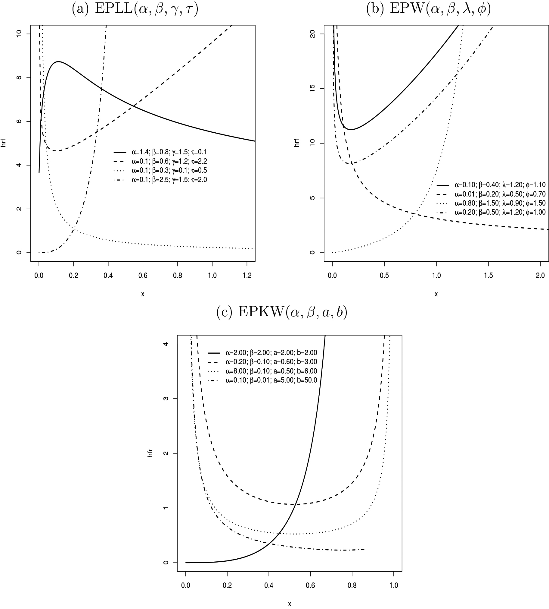
$\displaystyle h(x)=\frac{\beta\,g(x)\left\{-\log[1-G(x)]\right\}^{\beta-1}}{% \alpha^{\beta}\,[1-G(x)]}\exp\left[\left(\frac{-\log[1-G(x)]}{\alpha}\right)^{% \beta}\right]\,.$

Henceforth, $X\sim\text{EP-G}\,(\alpha,\beta,\bm{\theta})$ denotes a random variable with pdf Eq. (4), which has excellent flexibility and different hrf shapes, including the bathtub-shaped in Fig. 2, where the Weibull and log-logistic distributions do not have this shape.

The remainder of the article is structured as follows: Section 2 provides three EP-G sub-models. A linear representation for the pdf family Eq. (4) is derived in Section 3, and some of its structural properties are addressed in Section 4. The estimation of the parameters and a new regression model are reported in Sections 5 and 6, respectively. A simulation study is presented in Section 7. The potentiality of the new models is illustrated in two real-data applications in Section 8, and some conclusions are offered in Section 9.

2. Special distributions

This section provides three EP-G sub-models. All calculations are done using the R software (R Core Team, 2020).

2.1 Exponential power log-logistic (EPLL)

Consider the baseline log-logistic (LL) with two parameters $\gamma,\tau>0$ and cdf (for $x>0$ )

$\displaystyle G(x)=1-\left[1+\left(\frac{x}{\tau}\right)^{\gamma}\right]^{-1}\,.$

Then, the pdf from Eq. (4) and hrf of the EPLL model are

$\displaystyle f(x)=\frac{\beta\,\gamma\,\tau^{-\gamma}x^{\gamma-1}\left\{\log% \left[1+\left(\frac{x}{\tau}\right)^{\gamma}\right]\right\}^{\beta-1}}{\alpha^% {\beta}\,\left[1+\left(\frac{x}{\tau}\right)^{\gamma}\right]}\exp\left[\left(% \frac{\log\left[1+\left(\frac{x}{\tau}\right)^{\gamma}\right]}{\alpha}\right)^% {\beta}\right]\times\exp\left\{1-\exp\left[\left(\frac{\log\left[1+\left(\frac% {x}{\tau}\right)^{\gamma}\right]}{\alpha}\right)^{\beta}\right]\right\}$ (5)

and

$\displaystyle h(x)=\frac{\beta\,\gamma\,\tau^{-\gamma}x^{\gamma-1}\left\{\log% \left[1+\left(\frac{x}{\tau}\right)^{\gamma}\right]\right\}^{\beta-1}}{\alpha^% {\beta}\,\left[1+\left(\frac{x}{\tau}\right)^{\gamma}\right]}\exp\left[\left(% \frac{\log\left[1+\left(\frac{x}{\tau}\right)^{\gamma}\right]}{\alpha}\right)^% {\beta}\right]\,,$

respectively.

2.2 Exponential power Weibull (EPW)

The Weibull cdf with parameters $\lambda,\phi>0$ is (for $x>0$ )

$\displaystyle G(x)=1-\exp\left[-\left(\lambda x\right)^{\phi}\right]\,.$

Thus, the EPW density can be obtained from Eq. (4) as

$\displaystyle f(x)=\beta\,\alpha^{-\beta}\phi\,\lambda^{\phi\beta}x^{\phi\beta% -1}\exp\left\{\frac{(\lambda x)^{\phi\beta}}{\alpha^{\beta}}+1-\exp\left[\frac% {(\lambda x)^{\phi\beta}}{\alpha^{\beta}}\right]\right\}$

and its corresponding hrf has the form

$\displaystyle h(x)=\beta\,\alpha^{-\beta}\phi\,\lambda^{\phi\beta}x^{\phi\beta% -1}\exp\left[\frac{(\lambda x)^{\phi\beta}}{\alpha^{\beta}}\right]\,.$

2.3 Exponential power Kumaraswamy (EPKW)

The Kumaraswamy cdf (for $0<x<1$ , $a,b>0$ ) is

$\displaystyle G(x)=1-(1-x^{a})^{b}\,.$

Then, the pdf and hrf of the EPKW model are

$\displaystyle f(x)=\frac{\beta\,a\,b\,x^{a-1}\left\{-\log[(1-x^{a})^{b}]\right% \}^{\beta-1}}{\alpha^{-\beta}\,(1-x^{a})}\exp\left[\left(\frac{-\log[(1-x^{a})% ^{b}]}{\alpha}\right)^{\beta}\right]\times\exp\left\{1-\exp\left[\left(\frac{-% \log[(1-x^{a})^{b}]}{\alpha}\right)^{\beta}\right]\right\}$

and

$\displaystyle h(x)=\frac{\beta\,a\,b\,x^{a-1}\left\{-\log[(1-x^{a})^{b}]\right% \}^{\beta-1}}{\alpha^{-\beta}\,(1-x^{a})}\exp\left[\left(\frac{-\log[(1-x^{a})% ^{b}]}{\alpha}\right)^{\beta}\right]\,,$

respectively.

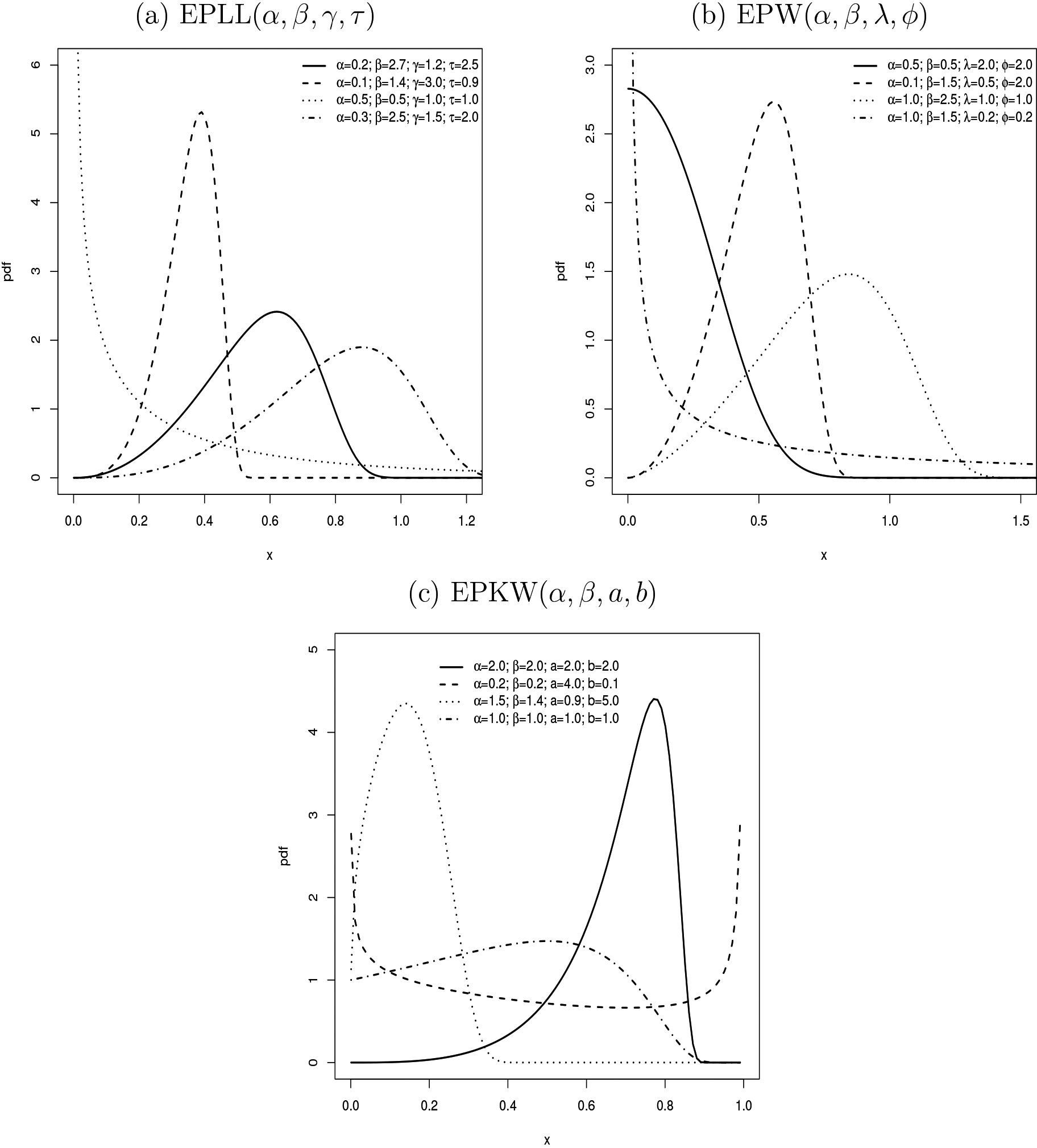
Figure 1 displays the EPLL, EPW, and EPKW densities for some parameters, which can model symmetric, right-skewed, and left-skewed data. Their hrfs are reported in Fig. 2, which have different shapes, including the bathtub-shaped.

Figure 1.

Some EP-G density shapes.

Figure 2.

Some EP-G hazard rate shapes.

3. Linear representation

Firstly, using Taylor expansion, the cdf of the EP-G family in Eq. (3) can be expressed as

$\displaystyle F(x)=-\sum^{\infty}_{i=1}\frac{\left\{1-\exp\left[\left(\frac{-% \log[1-G(x)]}{\alpha}\right)^{\beta}\right]\right\}^{i}}{i!}\,.$

Applying the binomial theorem to $\left\{1-\exp\left[\left(\frac{-\log[1-G(x)]}{\alpha}\right)^{\beta}\right]% \right\}^{i}$ ,

$\displaystyle F(x)=\sum^{\infty}_{i=1}\sum^{i}_{j=0}\frac{(-1)^{j+1}}{i!}% \binom{i}{j}\exp\left[j\left(\frac{-\log[1-G(x)]}{\alpha}\right)^{\beta}\right% ]\,.$

Again, using Taylor expansion in $\exp\left[j\left(\frac{-\log[1-G(x)]}{\alpha}\right)^{\beta}\right]$ ,

$\displaystyle F(x)=\sum^{\infty}_{i=1}\sum^{i}_{j=0}\sum^{\infty}_{k=0}\frac{(% -1)^{j+1}j^{k}}{i!k!\alpha^{\beta k}}\binom{i}{j}\left\{-\log[1-G(x)]\right\}^% {\beta k}\,.$ (6)

From the proposition 2 of Castellares and Lemonte (2015), we can written

$\displaystyle[-\log(1-\upsilon)]^{c}=\upsilon^{c}\,\sum_{m=0}^{\infty}p_{m}(c)% \,\upsilon^{m},$ (7)

where $c\in\text{I\!R}$ , $|\upsilon|<1$ , $p_{0}(c)=1$ , $p_{m}(c)=c\,\psi_{m-1}(m+c-1)$ for $m\geqslant 1$ , and the quantities $\psi_{0}(w)=1/2$ , $\psi_{1}(w)=(2+3w)/24$ , $\psi_{2}(w)=(w+w^{2})/48$ , etc., are the Stirling polynomials.

For any arbitrary $G(x)$ , the density of the exponentiated-G class (exp-G) with power parameter $\delta>0$ is defined as

$\displaystyle\pi_{\delta}(x)=\delta\,g(x)\,G(x)^{\delta-1}\,.$

See Table 1 of Tahir and Nadarajah (2015) for properties of various published distributions in the exp-G class, including well-known models such as exp-Weibull (Mudholkar & Srivastava, 1993), exp-gamma (Nadarajah & Gupta, 2007), and exp-Fréchet (Nadarajah and Kotz, 2003).

Applying Eq. (7) into Eq. (6), we get

$\displaystyle F(x)=\sum^{\infty}_{i=1}\sum^{i}_{j=0}\sum^{\infty}_{k,m=0}\frac% {(-1)^{j+1}j^{k}}{i!k!\alpha^{\beta k}}\binom{i}{j}p_{m}(\beta k)\,\,G(x)^{m+% \beta k}\,.$

writing $G(x)^{m+\beta k}=\left\{1-[1-G(x)]\right\}^{m+\beta k}$ and applying the binomial theorem twice,

$\displaystyle F(x)=\sum^{\infty}_{i=1}\sum^{i}_{j=0}\sum^{\infty}_{k,m=0}\frac% {(-1)^{j+1}j^{k}}{i!k!\alpha^{\beta k}}\binom{i}{j}p_{m}(\beta k)\sum^{\infty}% _{\ell=0}\sum^{\ell}_{b=0}\,(-1)^{\ell+b}\binom{m+\beta k}{\ell}\binom{\ell}{b% }\,G(x)^{b}\,.$ (8)

Replacing $\sum^{\infty}_{\ell=0}\sum^{\ell}_{b=0}$ by $\sum^{\infty}_{b=0}\sum^{\infty}_{\ell=b}$ and rearranging the terms in Eq. (8),

$\displaystyle F(x)=\sum^{\infty}_{b=0}\,\varphi_{b}\,G(x)^{b}\,,$ (9)

where

$\displaystyle\varphi_{b}=\varphi_{b}(\alpha,\beta)=\sum^{\infty}_{i=1}\sum^{i}% _{j=0}\sum^{\infty}_{k,m=0}\sum^{\infty}_{\ell=b}\frac{(-1)^{j+\ell+b+1}j^{k}}% {i!k!\alpha^{\beta k}}\binom{i}{j}\binom{m+\beta k}{\ell}\binom{\ell}{b}p_{m}(% \beta k)\,.$

By differentiating Eq. (9), the pdf of the EP-G family takes the form

$\displaystyle f(x)=\sum^{\infty}_{b=0}\varphi_{b+1}\,\pi_{b+1}(x)\,,$ (10)

where $\pi_{b+1}(x)$ is the exp-G density with power $b+1$ .

Hence, some mathematical properties of the EP-G family can be determined from Eq. (10) and those of the exp-G class.

4. Main properties

The quantile function (qf) of $X$ follows by inverting Eq. (3) as (for $0<u<1$ )

$\displaystyle Q_{X}(u)=Q_{X}(u;\alpha,\beta,\bm{\theta})=Q_{G}\left(1-\exp% \left\{-\alpha\sqrt[\beta]{\log\left[1-\log(1-u)\right]}\right\}\right)\,,$ (11)

where $Q_{G}(\cdot)=G^{-1}(\cdot)$ is the baseline qf. So, the EP-G observations for given $G(x)$ can be easily generated from Eq. (11). Further, the Bowley skewness (Kenney & Keeping, 1962) and Moors kurtosis (Moors, 1988) of this family are

$\displaystyle\mathcal{B}=\frac{Q_{X}(3/4)+Q_{X}(1/4)-2Q_{X}(1/2)}{Q_{X}(3/4)-Q% _{X}(1/4)}$

and

$\displaystyle\mathcal{M}=\frac{Q_{X}(7/8)-Q_{X}(5/8)+Q_{X}(3/8)-Q_{X}(1/8)}{Q_% {X}(6/8)-Q_{X}(2/8)}\,,$

respectively. Plots of these measures for the EPLL distribution as functions of $\beta$ ( $\alpha$ and $\gamma$ fixed and $\tau=0.1$ ) reported in Fig. 3 show that both measures decrease when $\beta$ increases.

Figure 3.

Bowley skewness and Moors kurtosis of the EPLL distribution.

The $s$ th ordinary moment of $X$ is $\mu^{\prime}_{s}=\text{I\!E}(X^{s})=\int^{\infty}_{-\infty}x^{s}f(x)\,\text{d}x$ . We can write from Eq. (10)

$\displaystyle\mu^{\prime}_{s}=\sum^{\infty}_{b=0}\varphi_{b+1}\,\text{I\!E}% \left(Y^{s}_{b+1}\right)=\sum^{\infty}_{b=0}\,\,(b+1)\,\varphi_{b+1}\,\int^{1}% _{0}\left[Q_{G}(u)\right]^{s}u^{b}\text{d}u\,,$

where $Y_{b+1}$ denotes the exp-G $\left(b+1\right)$ random variable.

The $s$ th incomplete moment $m_{s}(z)=\int^{z}_{-\infty}x^{s}f(x)\,\text{d}x$ of $X$ follows from Eq. (10) as

$\displaystyle m_{s}(z)=\sum^{\infty}_{b=0}\varphi_{b+1}\int^{z}_{-\infty}x^{s}% \pi_{b+1}(x)\,\text{d}x=\sum^{\infty}_{b=0}\,(b+1)\,\varphi_{b+1}\int^{G(z)}_{% 0}[Q_{G}(u)]^{s}u^{b}\text{d}u\,.$

For a given probability $\nu$ , the Bonferroni and Lorenz curves are

$\displaystyle B(\nu)=\frac{m_{1}(w)}{\nu\mu^{\prime}_{1}}\ \text{and}\ L(\nu)=% \frac{m_{1}(w)}{\mu^{\prime}_{1}}\,,$

respectively, where $w=Q_{X}(\nu)$ is determined from Eq. (11). Plots of these curves for the EPLL distribution versus $\nu$ for specific values of $\alpha$ and $\beta$ ( $\gamma=0.8$ and $\tau=1.5$ ) are reported in Fig. 4.

Figure 4.

Bonferroni and Lorenz curves of the EPLL distribution.

The generating function (gf) of $X$ can be determined from Eq. (10) as

$\displaystyle M_{X}(t)=\text{I\!E}(\text{e}^{tx})=\sum^{\infty}_{b=0}\varphi_{% b+1}\,M_{b+1}(t)=\sum^{\infty}_{b=0}\,\,(b+1)\,\varphi_{b+1}\,\int^{1}_{0}\exp% \left[t\,Q_{G}(u)\right]\,u^{b}\text{d}u\,,$

where $M_{b+1}(t)$ is the gf of $Y_{b+1}$ .

5. Estimation

The parameters of the new family are estimated utilizing the maximum likelihood method. Let $x_{1},\ldots,x_{n}$ be independent and identically distributed (iid) observations from the pdf Eq. (4). Then, the log-likelihood function for $\bm{\Theta}=(\alpha,\beta,\bm{\theta})^{\top}$ is

$\displaystyle\ell(\bm{\Theta})=n\,[\,\log(\beta)-\beta\log(\alpha)\,]+\sum^{n}% _{i=1}\log\,[\,g(x_{i})\,]-\sum^{n}_{i=1}\log\,[\,1-G(x_{i})\,]+(\beta-1)\sum^% {n}_{i=1}\log\,\{-\log[\,1-G(x_{i})\,]\}+\frac{1}{\alpha^{\beta}}\sum^{n}_{i=1% }\{-\log\,[\,1-G(x_{i})\,]\}^{\beta}+\sum^{n}_{i=1}\left\{1-\exp\left[\left(% \frac{-\log\,[\,1-G(x_{i})\,]}{\alpha}\right)^{\beta}\right]\right\}\,.$ (12)

The maximum likelihood estimate (MLE) can be determined by maximizing numerically Eq. (12) using the functions optim, MaxBFGS, or PROC NLMIXED in R, Ox, or SAS software, respectively.

6. Regression

Here, the log-exponential power log-logistic (LEPLL) random variable $Y$ is defined by the transformation $Y=\log(X)$ , where $X$ has pdf Eq. (5). The LEPLL density reparameterized by $\gamma=1/\sigma$ and $\tau=\text{e}^{\mu}$ has the form

$\displaystyle f(y)=\frac{\beta\,\text{e}^{\left(\frac{y-\mu}{\sigma}\right)}% \left\{\log\left[1+\text{e}^{\left(\frac{y-\mu}{\sigma}\right)}\right]\right\}% ^{\beta-1}}{\sigma\,\alpha^{\beta}\,\left[1+\text{e}^{\left(\frac{y-\mu}{% \sigma}\right)}\right]}\exp\left\{\left(\frac{\log\left[1+\text{e}^{\left(% \frac{y-\mu}{\sigma}\right)}\right]}{\alpha}\right)^{\beta}\right\}\times\exp% \left\{1-\exp\left[\left(\frac{\log\left[1+\text{e}^{\left(\frac{y-\mu}{\sigma% }\right)}\right]}{\alpha}\right)^{\beta}\right]\right\}\ y\in\text{I\!R},$ (13)

where $\alpha,\beta,\sigma>0$ and $\mu\in\text{I\!R}$ . Equation (13) has the location-scale form, where $\mu$ and $\sigma$ are location and scale parameters, respectively. Therefore, if $X\sim\text{EPLL}\,(\alpha,\beta,\gamma,\tau)$ , then $Y\sim\text{LEPLL}\,(\alpha,\beta,\mu,\sigma)$ .

The survival function referring to Eq. (13) and the density of $Z=(Y-\mu)/\sigma$ are

$\displaystyle S(y)=\exp\left\{1-\exp\left[\left(\frac{\log\left[1+\text{e}^{% \left(\frac{y-\mu}{\sigma}\right)}\right]}{\alpha}\right)^{\beta}\right]\right\}$

and

$\displaystyle f(z)=\frac{\beta\,\text{e}^{z}\left[\,\log\left(1+\text{e}^{z}% \right)\,\right]^{\beta-1}}{\alpha^{\beta}\,\left(1+\text{e}^{z}\right)}\exp% \left\{\left[\frac{\log\left(1+\text{e}^{z}\right)}{\alpha}\right]^{\beta}% \right\}\times\exp\left\{1-\exp\left[\left(\frac{\log\left[1+\text{e}^{z}% \right]}{\alpha}\right)^{\beta}\right]\right\},\ z\in\text{I\!R}\,.$ (14)

Equation (14) is the standard LEPLL density. In addition, we construct a regression model for the response variable $y_{i}$ and the explanatory variable vector $\bm{v}_{i}^{\top}=(v_{i1},\ldots,v_{ip})$ based on Eq. (13) as

$\displaystyle y_{i}=\bm{v}_{i}^{\top}\bm{\eta}+\sigma z_{i},\quad i=1,\ldots,n\,,$ (15)

where $\mu_{i}=\bm{v}^{\top}_{i}\bm{\eta}$ , $\bm{\eta}=(\eta_{1},\ldots,\eta_{p})^{\top}$ is the $p$ vector of unknown coefficients, and $z_{i}$ is the random error with density function Eq. (14).

The survival and density functions of $Y_{i}$ are

$\displaystyle S(y_{i})=\exp\left\{1-\exp\left[\left(\frac{\log\left[1+\text{e}% ^{z_{i}}\right]}{\alpha}\right)^{\beta}\right]\right\}$

and

$\displaystyle f(y_{i})=\frac{\beta\,\text{e}^{z_{i}}\left[\,\log\left(1+\text{% e}^{z_{i}}\right)\,\right]^{\beta-1}}{\sigma\,\alpha^{\beta}\,\left(1+\text{e}% ^{z_{i}}\right)}\exp\left\{\left[\frac{\log\left(1+\text{e}^{z_{i}}\right)}{% \alpha}\right]^{\beta}\right\}\times\exp\left\{1-\exp\left[\left(\frac{\log% \left[1+\text{e}^{z_{i}}\right]}{\alpha}\right)^{\beta}\right]\right\}\,,$

respectively, where $z_{i}=(y_{i}-\bm{v}_{i}^{\top}\bm{\eta})/\sigma$ .

Let $Y_{i}$ be the lifetime and $C_{i}$ be the non-informative censoring time, assuming that $Y_{i}$ and $C_{i}$ are independent random variables, and $y_{i}=\min(Y_{i},C_{i})$ . The log-likelihood function for $\bm{\theta}=(\alpha,\beta,\sigma,\bm{\eta}^{\top})^{\top}$ from the regression model Eq. (15) (for right censored data) has the form

$\displaystyle\ell(\bm{\theta})=d\,[\,\log(\beta)-\log(\sigma)-\beta\log(\alpha% )\,]+(\beta-1)\sum_{i\in F}\log\left[\,\log\left(1+\text{e}^{z_{i}}\right)\,% \right]-\sum_{i\in F}\log\left(1+\text{e}^{z_{i}}\right)+\sum_{i\in F}\left\{% \left[\frac{\log\left(1+\text{e}^{z_{i}}\right)}{\alpha}\right]^{\beta}\right% \}+\sum_{i\in F}\left\{1-\exp\left[\left(\frac{\log\left[1+\text{e}^{z_{i}}% \right]}{\alpha}\right)^{\beta}\right]\right\}+\sum_{i\in C}\left\{1-\exp\left% [\left(\frac{\log\left[1+\text{e}^{z_{i}}\right]}{\alpha}\right)^{\beta}\right% ]\right\}\,,$ (16)

where $d$ is the number of failures, $F$ and $C$ are sets of uncensored and censored observations, respectively. Equation (16) reduces to the usual log-likelihood for $d=n$ and $y_{i}\in F\,\,\forall i$ .

The MLE $\bm{\widehat{\theta}}$ of $\bm{\theta}$ is calculated by maximizing numerically Eq. (16) using R, Ox, or SAS software.

7. Simulations

A first simulation study is done to check the accuracy of the MLEs in the EPLL distribution under three different scenarios. We perform one thousand Monte Carlo trials using the log-logistic qf in Eq. (11) for four sample sizes $(n=50,100,200,500)$ . The average estimates (AEs), biases, and mean squared errors (MSEs) calculated in Table 1 show that the AEs converge to the true values of the parameters and that the biases and MSEs tend to zero when $n$ increases.

Table 1
Simulation results from the EPLL distribution

		(1.8, 0.4, 5.3, 7.8)						(1.7, 0.6, 1.6, 0.3)						(2.0, 0.8, 1.7, 0.2)
$n$	Par	AE		Bias		MSE		AE		Bias		MSE		AE		Bias		MSE
50	$\alpha$	3	.358	1	.558	23	.710	3	.654	1	.954	26	.249	5	.097	3	.097	49	.876
	$\beta$	0	.662	0	.262	0	.379	1	.103	0	.503	0	.962	1	.362	0	.562	1	.189
	$\gamma$	5	.879	0	.579	8	.040	1	.963	0	.363	1	.838	2	.576	0	.876	4	.464
	$\tau$	6	.938	$-$ 0	.861	8	.090	0	.267	$-$ 0	.032	0	.110	0	.179	$-$ 0	.020	0	.050
ANI		31.7077						31.3941						33.5482
100	$\alpha$	2	.357	0	.557	5	.901	2	.395	0	.695	5	.004	3	.287	1	.287	13	.443
	$\beta$	0	.542	0	.142	0	.138	0	.889	0	.289	0	.386	1	.133	0	.333	0	.513
	$\gamma$	5	.361	0	.061	3	.442	1	.689	0	.089	0	.586	2	.013	0	.313	1	.129
	$\tau$	7	.156	$-$ 0	.643	4	.107	0	.274	$-$ 0	.025	0	.061	0	.182	$-$ 0	.017	0	.024
ANI		16.4643						18.6651						18.3673
200	$\alpha$	1	.939	0	.139	0	.358	1	.956	0	.256	0	.613	2	.449	0	.449	1	.906
	$\beta$	0	.451	0	.051	0	.020	0	.738	0	.138	0	.123	0	.982	0	.182	0	.212
	$\gamma$	5	.239	$-$ 0	.060	1	.389	1	.597	$-$ 0	.002	0	.204	1	.768	0	.068	0	.258
	$\tau$	7	.498	$-$ 0	.301	0	.006	0	.275	$-$ 0	.024	0	.027	0	.183	$-$ 0	.016	0	.013
ANI		7.8456						12.6940						14.5364
500	$\alpha$	1	.852	0	.052	0	.126	1	.786	0	.086	0	.165	2	.142	0	.142	0	.288
	$\beta$	0	.421	0	.026	0	.006	0	.652	0	.052	0	.031	0	.876	0	.076	0	.064
	$\gamma$	5	.252	$-$ 0	.047	0	.538	1	.586	$-$ 0	.013	0	.074	1	.702	0	.002	0	.079
	$\tau$	7	.680	$-$ 0	.119	0	.546	0	.289	$-$ 0	.010	0	.011	0	.191	$-$ 0	.008	0	.005
ANI		6.6297						9.3544						11.7072

For the second simulation, the observations $y_{1},\ldots,y_{n}$ are generated from $Y_{i}\sim\text{LEPLL}\,(\alpha,\beta,\sigma,\mu_{i})$ , where $\mu_{i}=\eta_{0}+\eta_{1}v_{i1}$ , and $v_{i1}$ is obtained from a uniform $(0,1)$ distribution. The precision of the MLEs is investigated for $1,000$ samples by taking $\alpha=1.8,\beta=0.4,\sigma=0.6,\eta_{0}=1.7$ , $\eta_{1}=0.2$ , and $n=50,100,200$ , and $500$ . A uniform distribution $(0,b)$ is also used to generate the censoring times $c_{1},\ldots,c_{n}$ , where $b$ determines the censoring percentage (0%, 10%, 30%). The censoring indicator $\delta_{i}=1$ if $y_{i}\leqslant c_{i}$ and $\delta_{i}=0$ otherwise, and $y^{*}_{i}=\min(y_{i},c_{i})$ provides the observed times.

Table 2

Simulation results from the LEPLL regression model

		0%						10%						30%
$n$	Par	AE		Bias		MSE		AE		Bias		MSE		AE		Bias		MSE
50	$\alpha$	2	.370	0	.570	4	.928	2	.420	0	.620	5	.697	2	.752	0	.952	12	.942
	$\beta$	0	.588	0	.188	0	.287	0	.560	0	.160	0	.414	0	.524	0	.124	0	.803
	$\sigma$	0	.690	0	.090	0	.278	0	.635	0	.035	0	.368	0	.603	0	.003	1	.002
	$\eta_{0}$	1	.261	$-$ 0	.438	2	.458	1	.367	$-$ 0	.332	2	.812	1	.571	$-$ 0	.128	3	.151
	$\eta_{1}$	0	.195	$-$ 0	.004	1	.183	0	.227	0	.027	1	.152	0	.244	0	.044	1	.080
ANI		36.855						36.863						35.365
100	$\alpha$	2	.058	0	.258	1	.238	2	.173	0	.373	1	.977	2	.374	0	.574	4	.317
	$\beta$	0	.508	0	.108	0	.108	0	.560	0	.160	0	.238	0	.578	0	.178	0	.433
	$\sigma$	0	.657	0	.057	0	.085	0	.671	0	.071	0	.139	0	.664	0	.064	0	.329
	$\eta_{0}$	1	.403	$-$ 0	.296	1	.185	1	.301	$-$ 0	.398	2	.116	1	.295	$-$ 0	.404	2	.683
	$\eta_{1}$	0	.179	$-$ 0	.020	0	.532	0	.169	$-$ 0	.030	0	.649	0	.184	0	.015	0	.664
ANI		14.225						21.724						25.760
200	$\alpha$	1	.936	0	.136	0	.462	1	.967	0	.167	0	.657	2	.071	0	.271	0	.983
	$\beta$	0	.443	0	.043	0	.027	0	.470	0	.070	0	.062	0	.515	0	.115	0	.175
	$\sigma$	0	.622	0	.022	0	.022	0	.640	0	.040	0	.047	0	.656	0	.056	0	.114
	$\eta_{0}$	1	.552	$-$ 0	.147	0	.413	1	.491	$-$ 0	.208	0	.657	1	.381	$-$ 0	.318	1	.277
	$\eta_{1}$	0	.199	$-$ 0	.000	0	.226	0	.185	$-$ 0	.014	0	.266	0	.176	$-$ 0	.023	0	.341
ANI		7.667						8.393						10.559
500	$\alpha$	1	.832	0	.032	0	.132	1	.835	0	.035	0	.159	1	.853	0	.053	0	.223
	$\beta$	0	.417	0	.017	0	.006	0	.426	0	.026	0	.012	0	.435	0	.035	0	.027
	$\sigma$	0	.613	0	.013	0	.008	0	.620	0	.020	0	.016	0	.626	0	.026	0	.035
	$\eta_{0}$	1	.654	$-$ 0	.045	0	.121	1	.629	$-$ 0	.070	0	.168	1	.612	$-$ 0	.087	0	.236
	$\eta_{1}$	0	.198	$-$ 0	.001	0	.084	0	.206	0	.006	0	.091	0	.207	0	.007	0	.101
ANI		7.166						7.304						8.182

The findings in Table 2 reveal that the AEs converge to the true parameter values and the biases and MSEs decay when $n$ increases, thus proving the consistency of the estimators. In general, the AEs, biases, and MSEs become larger as $b$ increases.

These simulations were performed using a script in R with the function optim using the quasi-Newton method (BFGS), which has a maximum limit of 100 interactions by default. We calculate the average number of interactions (ANI) at each sample size considering the scenarios in Tables 1 and 2, which indicate that the ANI decreases when $n$ increases and that the ANI increases when the censoring percentage increases. The choice of the parameters for the distribution is done in order to achieve a faster simulation speed. The simulation process is slower when the parameters $\alpha<1$ and $\beta>1$ .

8. Applications

The potential of the proposed family is evaluated on two data sets for the log-logistic as the baseline distribution. The Cramér-von Mises $(W^{*})$ , Anderson-Darling $(A^{*})$ , Akaike information criterion (AIC), Consistent Akaike information criterion (CAIC), Bayesian information criterion (BIC), Hannan-Quinn information criterion (HQIC), and Kolmogorov-Smirnov (KS) (with its $p$ -value) are chosen to compare the fitted models. All calculations in Section 8.1 are determined via the AdequacyModel package (Marinho et al., 2019) in R software, and the optim function is used in a script in R to produce all the results in Section 8.2.

8.1 COVID-19 data

The data set corresponds to the recovery times (in days) of patients diagnosed with COVID-19 in the city of Cuiabá (Brazil) in 2020. This study consists of 70 infected individuals confirmed by laboratory tests. The recovery time is defined as the period between the onset of symptoms and the cure of the disease. This data set are: 34, 33, 43, 33, 75, 33, 47, 48, 52, 53, 56, 41, 58, 58, 37, 55, 31, 59, 43, 43, 42, 43, 43, 30, 63, 32, 30, 30, 26, 43, 82, 31, 69, 32, 45, 45, 35, 34, 37, 64, 25, 28, 71, 62, 34, 44, 53, 47, 74, 42, 54, 27, 49, 44, 65, 44, 45, 50, 70, 71, 37, 66, 67, 36, 53, 37, 47, 37, 42, 32. See http://www.saude.mt.gov.br/painelcovidmt2.

Some descriptive statistics for these data include: mean $=$ 46.30, median $=$ 43.50, standard deviation $=$ 13.78, skewness $=$ 0.60, kurtosis $=$ 2.49, minimum $=$ 25, and maximum $=$ 82.

Next, the EPLL distribution is compared with seven other models widely studied in the literature, namely, the beta log-logistic (BLL) (Lemonte, 2014), Kumaraswamy log-logistic (KLL) (De Santana et al., 2012), beta Weibull (BW) (Lee et al., 2007), Kumaraswamy Weibull (KW) (Cordeiro et al., 2010), gamma Burr XII (GBXII) (Guerra et al., 2017), gamma log-logistic (GLL) (Ramos et al., 2013), and gamma Weibull (GW) (Nadarajah et al., 2015) models.

Table 3
Findings from the fitted models to COVID-19 data

Model	MLEs (SEs)
EPLL $(\alpha,\beta,\gamma,\tau)$	25.22	1.65	28.25	24.18
	(1.12)	(0.17)	(0.02)	(0.01)
BLL $(a,b,\gamma,\tau)$	31.41	9.49	1.28	17.01
	(86.86)	(20.97)	(1.34)	(39.81)
KLL $(a,b,\gamma,\tau)$	30.36	5.07	1.86	10.53
	(73.74)	(6.39)	(0.93)	(16.83)
BW $(a,b,\alpha,\beta)$	28.14	0.12	0.06	2.11
	(11.58)	(0.02)	(0.01)	(0.05)
KW $(a,b,\alpha,\beta)$	7.07	0.14	2.61	0.04
	(0.06)	(0.04)	(0.02)	(0.01)
GBXII $(a,\gamma,k,\tau)$	18.92	9.47	1.54	12.14
	(2.10)	(0.22)	(0.17)	(0.20)
GLL $(a,\gamma,\tau)$	18.58	12.27	14.46
	(0.84)	(0.50)	(0.39)
GW $(a,\alpha,\beta)$	18.36	0.79	1.18
	(1.93)	(0.04)	(0.27)

Table 3 lists the MLEs and their respective standard errors (SEs) in parentheses of the fitted distributions to the current data. The estimates are accurate for the EPLL, BW, KW, GBXII, GLL, and GW distributions. In contrast, the SEs for the BLL and KLL distributions are higher compared to their estimates. The EPLL distribution has the lowest values of the adequacy measures in Table 4.

Table 4

Some measures of the fitted models to COVID-19 data

Model	$W^{*}$	$A^{*}$	AIC	CAIC	BIC	HQIC	KS	$p$ -value
EPLL	0.05	0.30	560.39	561.00	569.38	563.96	0.07	0.89
BW	0.06	0.32	561.66	562.27	570.65	565.23	0.08	0.74
KW	0.07	0.45	563.49	564.11	572.49	567.07	0.09	0.60
GBXII	0.07	0.46	565.12	565.74	574.12	568.69	0.08	0.69
GLL	0.07	0.46	563.48	563.49	569.87	565.80	0.08	0.68
GW	0.09	0.61	564.56	564.93	571.31	567.25	0.09	0.56

Table 5

Findings from the fitted regression to AIDS data and the adequacy measures

	LEPLL		LGL		Logistic
Parameter	MLE (SE)		MLE (SE)		MLE (SE)
$\alpha$	0	.90 (0.34)	$-$ ( $-$ )		$-$ ( $-$ )
$\beta$	0	.18 (0.03)	0	.69 (0.10)	$-$ ( $-$ )
$\sigma$	0	.20 (0.03)	0	.84 (0.22)	0	.74 (0.06)
$\eta_{0}$	7	.88* (0.05)	7	.30* (0.44)	7	.08* (0.28)
$\eta_{1}$	1	.17* (0.03)	1	.16* (0.17)	1	.16* (0.17)
$\eta_{2}$	$-$ 1	.23* (0.05)	$-$ 1	.17* (0.18)	$-$ 1	.17* (0.18)
AIC	410.58		410.94		411.31
CAIC	411.03		411.72		412.10
BIC	423.63		430.51		430.89
HQIC	415.86		418.86		419.24

${}^{*}p$ -value $<$ 0.0001.

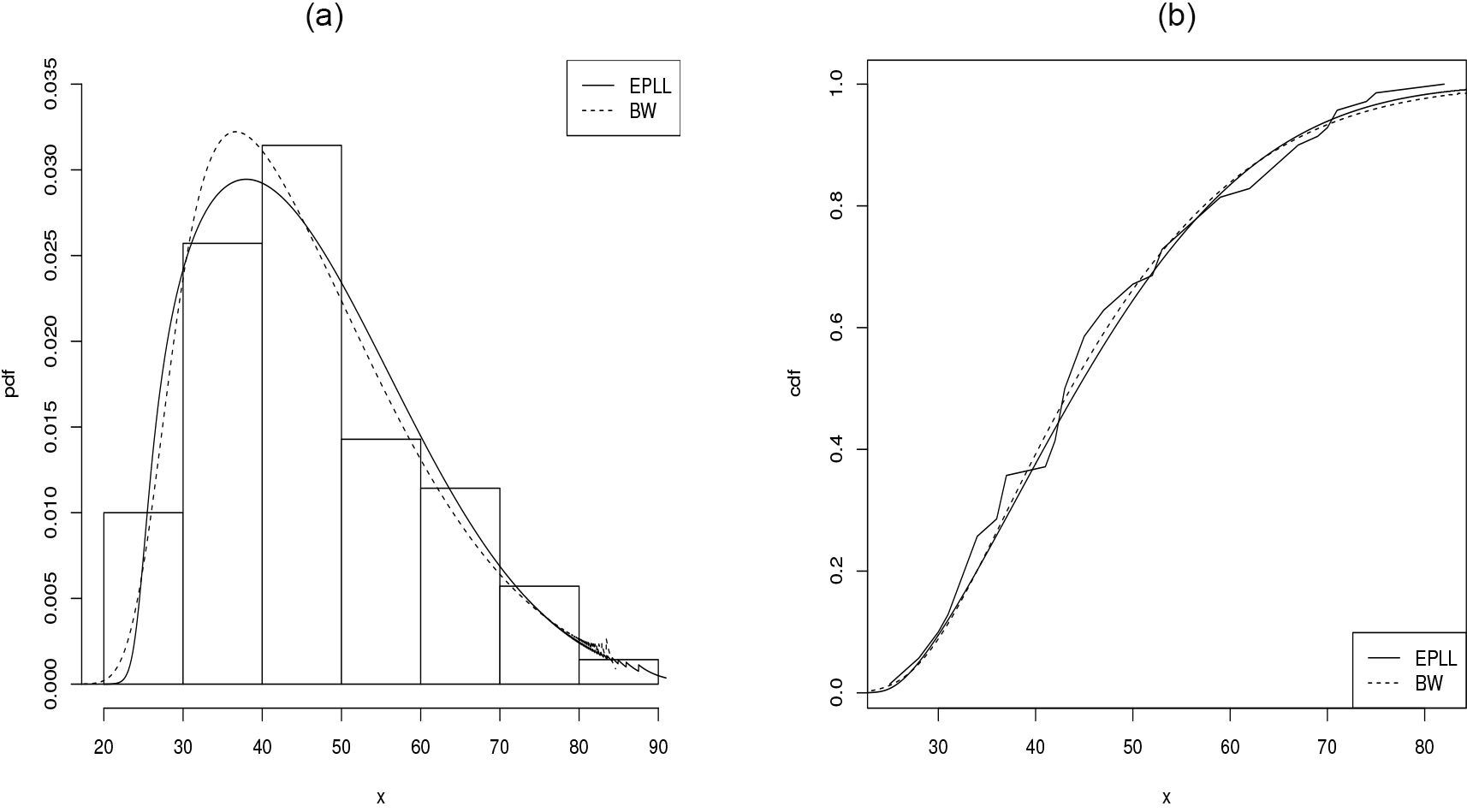
Figure 5 shows that the estimated pdf and cdf of the EPLL distribution are closer to the histogram and the empirical cdf, respectively. Based on these results, the EPLL distribution provides the best fit for these data.

Figure 5.

(a) Estimated pdfs, (b) estimated cdfs and the empirical cdf.

8.2 AIDS data

We consider 193 individuals diagnosed with AIDS treated at the Instituto de Pesquisa Clínica Evandro Chagas (IPEC-FIOCRUZ) between 1986 and 2002. These data can be downloaded directly from the link http://sobrevida. fiocruz.br/aidsclassico.html. The analysis does not include individuals younger than 13 years of age or with less than 15 days of follow-up. See Campos et al. (2005) for a complete exploratory data analysis.

Survival time (in months) is the period elapsed from the date of AIDS diagnosis to the date of death (failure) or last attendance. Deaths not related to AIDS were considered censoring times (0 $=$ censored and 1 $=$ observed lifetime). The censoring percentage is 53.33%. The explanatory variable $v_{1}$ denotes the antiretroviral therapy (0 $=$ none, 1 $=$ mono, 2 $=$ combined, 3 $=$ potent) and the explanatory variable $v_{2}$ represents the type of follow-up (0 $=$ outpatient/day hospital, 1 $=$ later admission, 2 $=$ immediate admission).

The proposed regression model for these data has the form

$\displaystyle y_{i}=\eta_{0}+\eta_{1}v_{i1}+\eta_{2}v_{i2}+\sigma z_{i},\quad i% =1,\ldots,193\,,$

where $z_{i}$ has density Eq. (14). The results are compared with the log-gamma logistic (Hashimoto et al., 2017) and logistic regression models. Table 5 provides the MLEs, SEs in parentheses, $p$ -values, and adequacy measures for the three regression models fitted to the AIDS data. The estimates determined by the three regression models are accurate. The explanatory variables $v_{1}$ and $v_{2}$ are statistically significant for all models, thus meaning that antiretroviral therapy tends to prolong the failure times of patients. On the other hand, the negative sign of $\eta_{2}$ indicates that the greater the need for admission, the shorter the failure time.

The adequacy measures indicate that the LEPLL regression model is the best model among the three. Further, we use the generalized LR test (GLR) ((Vuong, 1989)) given by

$\displaystyle T_{\textit{LR,NN}}=\frac{1}{\widehat{\omega}^{2}\sqrt{n}}\sum^{n% }_{i=1}{\log}\frac{f(y_{i}|\bm{x}_{i},\hat{\bm{\theta}})}{g(y_{i}|\bm{x}_{i},% \hat{\bm{\gamma}})}\,,$ (17)

where

$\displaystyle\widehat{\omega}^{2}=\frac{1}{n}\sum^{n}_{i=1}\left[{\log}\frac{f% (y_{i}|\bm{x}_{i},\hat{\bm{\theta}})}{g(y_{i}|\bm{x}_{i},\hat{\bm{\gamma}})}% \right]^{2}-\left[\frac{1}{n}\sum^{n}_{i=1}\log\frac{f(y_{i}|\bm{x}_{i},\hat{% \bm{\theta}})}{g(y_{i}|\bm{x}_{i},\hat{\bm{\gamma}})}\right]^{2}$

is an estimate of the variance of Eq. (17), $f(y_{i}|\bm{x}_{i},\hat{\bm{\theta}})$ and $g(y_{i}|\bm{x}_{i},\hat{\bm{\gamma}})$ correspond to the estimated densities. If $n\rightarrow\infty$ , $T_{\textit{LR,NN}}\overset{D}{\rightarrow}N(0,1)$ . Thus, the null hypothesis is not rejected at significance level $\alpha$ if $|T_{\textit{LR,NN}}|\,\,\leqslant z_{\alpha/2}$ . In the first case, $f$ and $g$ denote the LEPLL and LGL regressions, respectively, which yields $T_{\textit{LR,NN}}=7.668$ . In the second case, $f$ and $g$ are the LEPLL and logistic regressions, respectively, yielding $T_{\textit{LR,NN}}=8.551$ . Therefore, the null hypothesis is rejected for $\alpha=0.05$ in favor of the LEPLL regression in both cases, confirming the results of Table 5.

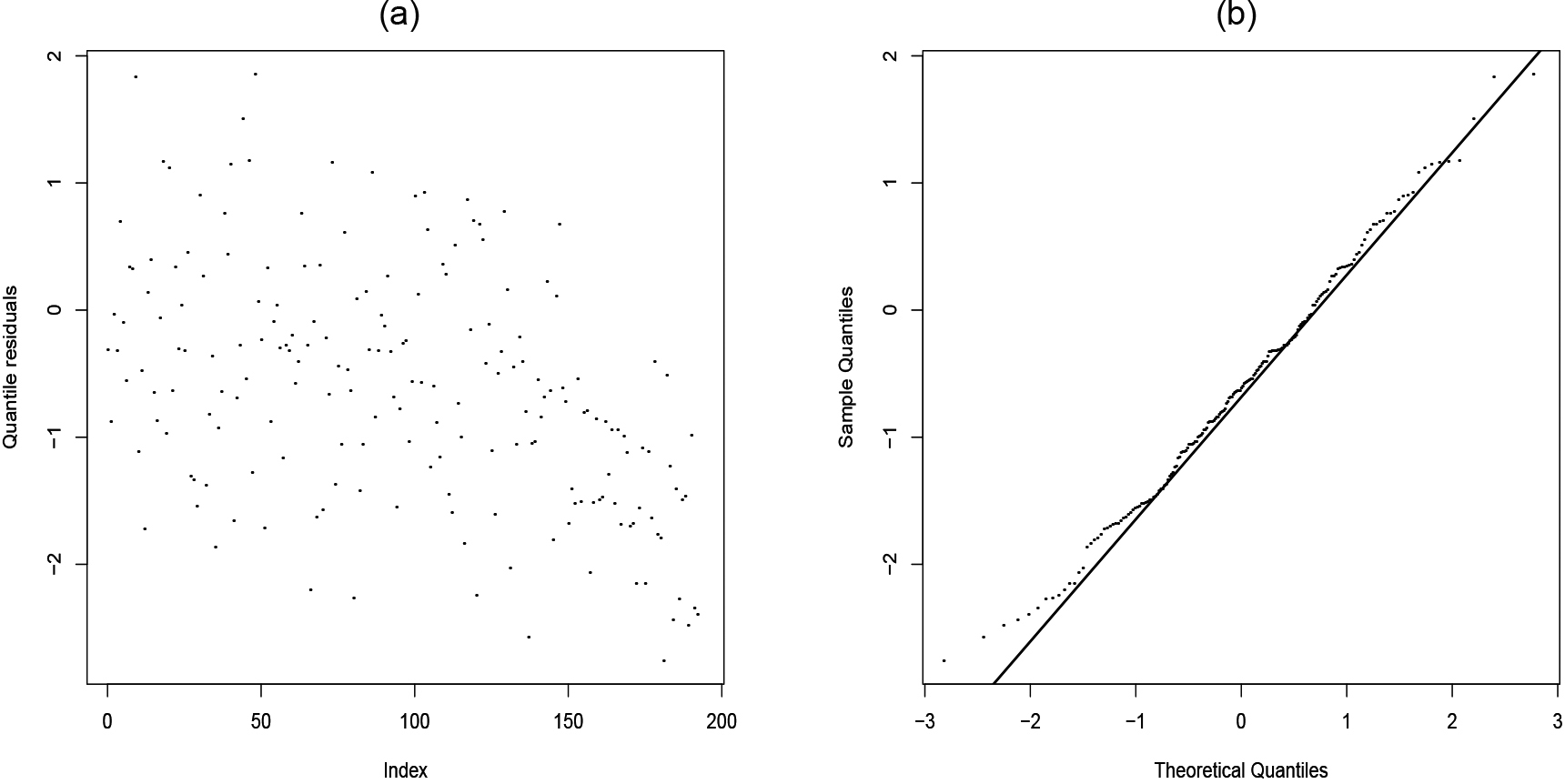
For a residual analysis of this fitted regression, we adopt the quantile residuals (qrs) (Dunn & Smyth, 1996), namely

$\displaystyle qr_{i}=\Phi^{-1}\left(1-\exp\left\{1-\exp\left[\left(\frac{\log% \left[1+\text{e}^{\hat{z}_{i}}\right]}{\hat{\alpha}}\right)^{\hat{\beta}}% \right]\right\}\right)\,,$

where $\Phi^{-1}(\cdot)$ is the standard normal qf and $\hat{z}_{i}=(y_{i}-\bm{v}_{i}^{\top}\bm{\hat{\eta}})/\hat{\sigma}$ . The residual index plot reported in Fig. 6(a) reveals that the qrs are randomly distributed and that no observations are outside the [ $-$ 3.3] range. The normal probability plot for the qrs in Fig. 6(b) indicates that the residuals approximately follow a standard normal distribution. Hence, there is no evidence against the LEPLL regression assumptions for this data set.

Figure 6.

(a) Index plot and (b) normal probability plot of the qrs.

9. Conclusions

We defined the exponential power-G family of distributions and discussed some of its mathematical properties. Also, we constructed a new log-exponential power log-logistic regression model. The simulation results reveal that the maximum likelihood estimators are consistent. Two applications to real data indicated that the new models obtained by the new family of distributions are competitive compared to the models generated by the beta-G, gamma-G, and Kumaraswamy-G generators. As a result, this new family can generate promising distributions and may be attractive for practical applications in other areas.

Footnotes

Acknowledgments

This work was supported by the Fundação de Amparo C̀iência e Tecnologia do Estado de Pernambuco (FACEPE) [IBPG-1448-1.02/20]. The authors thank the associate editor and the anonymous referees for some comments that improved the original version of the paper.

References

Al-Babtain

A. A.

Shakhatreh

M. K.

Nassar

, & Afify

A. Z.

(2020). A new modified Kies family: Properties, estimation under complete and type-II censored samples, and engineering applications. Mathematics, 8, 1345.

Alexander

Cordeiro

G. M.

Ortega

E. M. M.

, & Sarabia

(2012). Generalized beta-generated distributions. Computational Statistics & Data Analysis, 56, 1880-1897.

Alizadeh

Emadi

Doostparast

Cordeiro

G. M.

Ortega

E. M. M.

, & Pescim

R. R.

(2015). A new family of distributions: the kumaraswamy odd log-logistic, properties and applications. Hacettepe Journal of Mathematics and Statistics, 44, 1491-1512. Alzaatreh et al., 2013 Alzaatreh, A., Lee, C., & Famoye, F. (2013). A new method for generating families of continuous distributions. METRON, 71, 63-79. Baharith and Alamoudi, 2021 Baharith, L. A., & Alamoudi, H. H. (2021). The Exponentiated Fréchet Generator of Distributions with Applications. Symmetry, 13, 572. Bourguignon et al., 2014 Bourguignon, M., Silva, R., & Cordeiro, G. M. (2014). The Weibull-G Family of Probability Distributions. Journal of Data Science, 12, 53-68. Campos et al., 2005 Campos, D. P., Ribeiro, S. R., Grinsztejn, B., Veloso, V. G., Valente, J. G., Bastos, F. I., Morgado, M. G., & Gadelha, A. J. (2005). Survival of AIDS patients using two case definitions, Rio de Janeiro, Brazil, 1986-2003. Aids, 19, S22-S26. Castellares and Lemonte, 2015 Castellares, F., & Lemonte, A. J. (2015). A new generalized Weibull distribution generated by gamma random variables. Journal of the Egyptian Mathematical Society, 23, 382-390. Chipepa et al., 2019 Chipepa, F., Oluyede, B. O., & Makubate, B. (2019). A new generalized family of odd Lindley-G distributions with application. International Journal of Statistics and Probability, 8, 1-22. Cordeiro et al., 2016 Cordeiro, G. M., Alizadeh, M., & Marinho, P. R. D. (2016). The type I half-logistic family of distributions. Journal of Statistical Computation and Simulation, 86, 707-728. Cordeiro et al., 2017 Cordeiro, G. M., Alizadeh, M., Ozel, G., Hosseini, B., Ortega, E. M. M., & Altun, E. (2017). The generalized odd log-logistic family of distributions: properties, regression models and applications. Journal of Statistical Computation and Simulation, 87, 908-932. Cordeiro and de Castro, 2011 Cordeiro, G. M., & de Castro, M. (2011). A new family of generalized distributions. Journal of Statistical Computation and Simulation, 81, 883-898. Cordeiro et al., 2013 Cordeiro, G. M., Ortega, E. M. M., & Cunha, D. C. C. (2013). The exponentiated generalized class of distributions. Journal of Data Science, 11, 1-27. Cordeiro et al., 2010 Cordeiro, G. M., Ortega, E. M. M., & Nadarajah, S. (2010). The Kumaraswamy Weibull distribution with application to failure data. Journal of the Franklin Institute, 347, 1399-1429. Cordeiro et al., 2014 Cordeiro, G. M., Ortega, E. M. M., Popović, B. V., & Pescim, R. R. (2014). The Lomax generator of distributions: Properties, minification process and regression model. Applied Mathematics and Computation, 247, 465-486. De Santana et al., 2012 De Santana, T. V. F., Ortega, E. M. M., Cordeiro, G. M., & Silva, G. O. (2012). The Kumaraswamy-log-logistic distribution. Journal of Statistical Theory and Applications, 11, 265-291. Dunn and Smyth, 1996 Dunn, P. K., & Smyth, G. K. (1996). Randomized quantile residuals. Journal of Computational and Graphical Statistics, 5, 236-244. Eugene et al., 2002 Eugene, N., Lee, C., & Famoye, F. (2002). Beta-normal distribution and its applications. Communications in Statistics – Theory and Methods, 31, 497-512. Guerra et al., 2017 Guerra, R. R., Peña-Ramírez, F. A., & Cordeiro, G. M. (2017). The gamma Burr XII Distributions: Theory and Applications. Journal of Data Science, 15, 467-494. Gupta et al., 1998 Gupta, R. C., Gupta, P. L., & Gupta, R. D. (1998). Modeling failure time data by lehman alternatives. Communications in Statistics – Theory and Methods, 27, 887-904. Hashimoto et al., 2017 Hashimoto, E. M., Ortega, E. M. M., Cordeiro, G. M., & Hamedani, G. (2017). The log-gamma-logistic regression model: Estimation, sensibility and residual analysis. Journal of Statistical Theory and Applications, 16, 547-564. Kenney and Keeping, 1962 Kenney, J., & Keeping, E. (1962). Moving averages. 3 edn. NJ: Van Nostrand. Lee et al., 2007 Lee, C., Famoye, F., & Olumolade, O. (2007). Beta-Weibull distribution: some properties and applications to censored data. Journal of Modern Applied Statistical Methods, 6, 17. Lemonte, 2014 Lemonte, A. J. (2014). The beta log-logistic distribution. Brazilian Journal of Probability and Statistics, 28, 313-332. Marinho et al., 2019 Marinho, P. R. D., Silva, R. B., Bourguignon, M., Cordeiro, G. M., & Nadarajah, S. (2019). AdequacyModel: An R package for probability distributions and general purpose optimization. PLOS ONE, 14, 1-30. Marshall and Olkin, 1997 Marshall, A. W., & Olkin, I. (1997). A new method for adding a parameter to a family of distributions with application to the exponential and Weibull families. Biometrika, 84, 641-652. Moors, 1988 Moors, J. J. A. (1988). A quantile alternative for kurtosis. Journal of the Royal Statistical Society. Series D (The Statistician), 37, 25-32. Mudholkar and Srivastava, 1993 Mudholkar, G. S., & Srivastava, D. K. (1993). Exponentiated Weibull family for analyzing bathtub failure-rate data. IEEE Transactions on Reliability, 42, 299-302. Nadarajah et al., 2015 Nadarajah, S., Cordeiro, G. M., & Ortega, E. M. M. (2015). The Zografosâ€“Balakrishnan-G family of distributions: Mathematical properties and applications. Communications in Statistics – Theory and Methods, 44, 186-215. Nadarajah and Gupta, 2007 Nadarajah, S., & Gupta, A. K. (2007). The exponentiated gamma distribution with application to drought data. Calcutta Statistical Association Bulletin, 59, 29-54. Nadarajah and Kotz, 2003 Nadarajah, S., & Kotz, S. (2003). The exponentiated Fréchet distribution. Interstat Electronic Journal, 14, 1-7. R Core Team, 2020 R Core Team (2020). R: A Language and Environment for Statistical Computing. R Foundation for Statistical Computing, Vienna, Austria.

Ramos

M. W. A.

Cordeiro

G. M.

Marinho

P. R. D.

Dias

C. R. B.

, & Hamedani

(2013). The Zografos-Balakrishnan Log-Logistic Distribution: Properties and Applications. Journal of Statistical Theory and Applications, 12, 225-244.

Reyad

Jamal

Othman

, & Hamedani

(2018). The transmuted Gompertz-G family of distributions: properties and applications. Tbilisi Mathematical Journal, 11, 47-67.

Smith

R. M.

, & Bain

L. J.

(1975). An exponential power life-testing distribution. Communications in Statistics, 4, 469-481.

Tahir

M. H.

, & Nadarajah

(2015). Parameter induction in continuous univariate distributions: Well-established G families. Anais da Academia Brasileira de Ciências, 87, 539-568.

Vuong

Q. H.

(1989). Likelihood ratio tests for model selection and non-nested hypotheses. Econometrica, 57, 307-333.

Zografos

, & Balakrishnan

(2009). On families of beta-and generalized gamma-generated distributions and associated inference. Statistical Methodology , 6, 344-362.

The exponential power-G family of distributions: Properties,simulations,regression modeling and applications

Abstract

Keywords

1. Introduction

2.1 Exponential power log-logistic (EPLL)

2.3 Exponential power Kumaraswamy (EPKW)

Table 1 Simulation results from the EPLL distribution

8.1 COVID-19 data

Table 3 Findings from the fitted models to COVID-19 data

Footnotes

Acknowledgments

References

Table 1
Simulation results from the EPLL distribution

Table 3
Findings from the fitted models to COVID-19 data