Exact higher-order moments for linear non-homogeneous stochastic differential equation

Abstract

This paper investigates the moments of a stochastic process that satisfies the one-dimensional linear stochastic differential equation (SDE) with nonlinear time-dependent drift and diffusion coefficients. The goal is to derive formulas for the $n^{\text{th}}$ exact moment, that instead of seeking the transition density function by solving the Fokker-Plank equations or moment-generating functions, which can be difficult to solve in closed form. We will appropriately apply Itô’s formula and the properties of the Wiener process with a constant drift and diffusion term, which is a Gaussian process to obtain the exact higher-order moments.

Keywords

Higher-order moments stochastic differential equation time-dependent coefficients Itô’s formula

1. Introduction

In this paper we consider a stochastic process $\{X_{t},t\geqslant 0\}$ governed by linear stochastic differential equation (SDE) with nonlinear time-dependent coefficients:

$\displaystyle dX_{t}=\underbrace{\left(\alpha{\displaystyle\frac{g^{(k+1)}(t)}% {g^{(k)}(t)}}X_{t}+\beta{g^{(k)}(t)}^{\alpha}\right)}_{\mu(x,t)}dt+\underbrace% {\vphantom{{\displaystyle\frac{g^{(k+1)}(t)}{g^{(k)}(t)}}}\gamma{g^{(k)}(t)}^{% \alpha}}_{\sigma(t)}dW_{t}$ (1)

where $\{W_{t},t\geqslant 0\}$ denotes a one-dimensional standard Wiener process (or Brownian motion) with independent and identically Gaussian distributed (i.i.d) increments $W_{t}-W_{s}\sim\mathcal{N}(0,t-s)$ for all $t>s\geqslant 0$ . The time-dependent drift $\mu(x,t)$ and diffusion $\sigma(t)$ terms are known functions. The parameters $\alpha,\beta\in\mathbb{R}$ and $\gamma>0$ . We assume that $g(t)$ is piecewise continuous function on $(-\infty,+\infty)$ and $g^{(k)}(t)$ is $k^{\text{th}}$ derivative of $g(t)$ , where ${g^{(k)}(t)}\neq 0$ for all $t\in[0,+\infty[$ . The form of Eq. (1) contains some popular stochastic processes as its special cases. For instance, when $\alpha=0$ , the stochastic process becomes Merton (1973) model. When $\alpha\in\mathbb{Z}^{-}$ , $k\in\mathbb{Z}^{+}$ and $g(t)=\ln(t-T)$ , it becomes Brownian bridge process with time-dependent diffusion (see example 2). In addition, when $\alpha<0$ , $k=0$ and $g(t)=(t+1)$ , the model becomes the Vasicek (1977) process with mean $(\beta t+x_{0})g(t)^{\alpha}$ and variance $\gamma^{2}tg(t)^{2\alpha}$ . These models have a variety of applications in many disciplines and emerge naturally in the study of many phenomena. An example of this application is in financial modeling, including pricing of bond options, swaptions, modeling future interest short rates, and other interest rate derivatives (see e.g., Klebaner, 2005; Henderson& Plaschko, 2006; Alle, 2007; Mackevicius, 2016), as well as in many other fields of science and engineering.

In most cases, the density function or moment-generating function of a random variable is first acquired or specified. Then, either by integrating a power function along with the density function or by differentiating the moment-generating function are often used to obtain the moments. The higher-order moments of a stochastic process are very important because they provide information about the shape and spread of the distribution of the process. In particular, they can help characterize skewness and kurtosis of the distribution, as well as the estimation of diffusion models (see e.g., Bishwal, 2008, 2012). In most cases, the transition density function of linear non-homogeneous SDE may be determined by solving the corresponding Kolmogorov forward or Fokker-Planck equations (Risken, 1996). Even if the density or moment-generating functions can be established for certain exceptional circumstances, computing the moments would not be accessible if one desired high-order moments. In general, computing higher-order moments of a stochastic process satisfying a linear non-homogeneous SDE can be challenging, as the Fokker-Planck equation may not have an analytical solution. In such cases, numerical methods, such as Monte-Carlo simulations, may be used to approximate the moments of the process.

The main purpose of this paper is to investigate the exact higher-order moments of Eq. (1), which can provide important information about the statistical properties of this process, including its mean, variance, skewness, and kurtosis. Instead of seeking the density or moment-generating functions, we utilize Itô’s formula and the properties of the Wiener process with a constant drift and diffusion term. These formulas provide a simple computation of the $n^{\text{th}}$ exact moment. This leads to a very effective way to validate the performance of numerical simulations in stochastic modeling when applying the Eq. (1). Overall, by computing the higher-order moments of the process described by Eq. (1), researchers can gain a better understanding of its statistical properties and make more accurate predictions about its behavior over time.

The paper is structured into three main sections. In Section 2, we present the main results by deriving the exact formulas for the $n^{\text{th}}$ moment of Eq. (1). In Section 3, we perform a numerical Monte-Carlo simulation to calculate the moments of the propagation process and compare them with the analytical expressions derived in the previous section. Finally, we provide the conclusions of the paper in Section 4.

2. Main results

Suppose that $(\Omega,\mathcal{F},\mathbb{P})$ is a probability space. Let $\mathbb{X}=\{X_{t},t\geqslant 0\}$ be a stochastic process on $(\Omega,\mathcal{F},\mathbb{P})$ with state space $\mathbb{R}$ ; that is, $X_{t}$ takes values in $\mathbb{R}$ for all $t\geqslant 0$ . We consider the stochastic process $\mathbb{X}$ as the solution of the SDE:

$\displaystyle\left\{\begin{array}[]{l}dX_{t}=\left(\alpha{\displaystyle\frac{g% ^{(k+1)}(t)}{g^{(k)}(t)}}X_{t}+\beta{g^{(k)}(t)}^{\alpha}\right)dt+\gamma{g^{(% k)}(t)}^{\alpha}dW_{t}\\ X_{0}=x_{0}\end{array}\right.$ (2)

we assume that $X_{t}$ is well-defined for all $t\geqslant 0$ and $x_{0}\in\mathbb{R}$ can be either a random or a non-random initial condition independent of $W_{t}-W_{0}$ . The time-dependent drift $\mu(t,x)$ and diffusion $\sigma(t)$ coefficients which are assumed to be sufficiently regular (Lipschitz, bounded growth) for the existence and uniqueness the solution of Eq. (2) (see Oksendal, 2003). Throughout this paper we assume that all the moments of $X_{t}$ are finite. More precisely, we suppose $\mathbb{E}(X_{t}^{n})<\infty$ for all non-negative integer $n$ , where $\mathbb{E}(X_{t}^{0})\equiv 1$ . In what follows we consider a function $f(t,x)={g^{(k)}(t)}^{-\alpha}x$ and let $Y_{t}=f(t,X_{t})$ so that $Y_{t}$ is again an Itô process. by assuming $t_{0}=0$ , we applying Itô’s Lemma to $Y_{t}$ , which results in:

$\displaystyle dY_{t}=\beta dt+\gamma dW_{t}\Leftrightarrow Y_{t}=Y_{0}+\beta t% +\gamma W_{t}$ (3)

it is then easy to find the exact solution of Eq. (2):

$\displaystyle X_{t}={g^{(k)}(t)}^{\alpha}({g^{(k)}(0)}^{-\alpha}x_{0}+\beta t+% \gamma W_{t})$ (4)

it’s clear to find the moments of the process $X_{t}$ , we take expectation on both sides of Eq. (4).

.

Assume $g(t)$ is piecewise continuous function on $(-\infty,+\infty)$ and $\{\forall t\geqslant 0:{g^{(k)}(t)}\neq 0\}$ . The parameters $\alpha,\beta\in\mathbb{R}$ and $\gamma>0$ . For all non-negative integer $n$ , the exact high-order moments of Eq. (2) are given by:

$\displaystyle\mathbb{E}(X_{t}^{n})=\left\{\begin{array}[]{ll}x_{0}^{n}&\text{% if }t=0\\ \Psi(t)\text{H}_{n}(\Theta(t))t^{{\textstyle\frac{n}{2}}}&\text{if }t>0\end{% array}\right.$ (5)

where $\text{H}_{n}(x)$ is the $n^{\text{th}}$ Hermite polynomial evaluated at $x$ (see e.g., Olver et al., 2010, p. 438). The functions $\Psi(t)$ and $\Theta(t)$ satisfies the following expressions:

$\displaystyle\Psi(t)=2^{-{\textstyle\frac{n}{2}}}\left(\frac{\gamma{g^{(k)}(t)% }^{\alpha}}{\mathrm{i}}\right)^{n}\quad\text{and}\quad\Theta(t)=\frac{\left({g% ^{(k)}(0)}^{-\alpha}x_{0}+\beta t\right)\mathrm{i}}{\gamma\sqrt{2t}}$

in which $\mathrm{i}=\sqrt{-1}$ .

Proof..

From the Eq. (3), the stochastic process $Y_{t}$ is called a Wiener process with constant drift, which has the mean $\mu_{t}=y_{0}+\beta t$ and variance $\sigma^{2}_{t}=\gamma^{2}t$ . We see that $Y_{t}\mid Y_{0}=y_{0}$ has a Gaussian distribution:

$\displaystyle Y_{t}\mid Y_{0}=y_{0}\sim\mathcal{N}(y_{0}+\beta t,\gamma^{2}t)$

for a non-negative integer $n$ , the exact higher-order moments of $Y_{t}$ which are given by (see Willink, 2005):

$\displaystyle\mathbb{E}(Y_{t}^{n})=\left\{\begin{array}[]{ll}y_{0}^{n}&\text{% if }t=0\\ 2^{-{\textstyle\frac{n}{2}}}\left({\displaystyle\frac{\sigma_{t}}{\mathrm{i}}}% \right)^{n}\text{H}_{n}\left({\displaystyle\frac{\mu_{t}}{\sqrt{2}\sigma_{t}}}% \mathrm{i}\right)&\text{if }t>0\end{array}\right.$

then, we will apply the following change of variable to find the moments of Eq. (2):

$\displaystyle y={g^{(k)}(t)}^{-\alpha}x\Leftrightarrow x={g^{(k)}(t)}^{\alpha}y$ $\displaystyle\Leftrightarrow x^{n}=(g^{(k)}(t))^{\alpha n}y^{n}$

therefore we get:

$\displaystyle\mathbb{E}(X_{t}^{n})=(g^{(k)}(t))^{\alpha n}\mathbb{E}(Y_{t}^{n})$

hence, we plug the last expression into higher-order moments of $Y_{t}$ we obtain:

$\displaystyle\mathbb{E}(X_{t}^{n})=\left\{\begin{array}[]{ll}x_{0}^{n}&\text{% if }t=0\\ 2^{-{\textstyle\frac{n}{2}}}\left({\displaystyle\frac{{g^{(k)}(t)}^{\alpha}% \sigma_{t}}{\mathrm{i}}}\right)^{n}\text{H}_{n}\left({\displaystyle\frac{\mu_{% t}}{\sqrt{2}\sigma_{t}}}\mathrm{i}\right)&\text{if }t>0\end{array}\right.$

by inserting the expression of $\mu_{t}$ (with $y_{0}={g^{(k)}(0)}^{-\alpha}x_{0}$ ) and $\sigma_{t}$ into last equation the proof is completed. ∎

.

For a non-negative integer $n$ , the higher-order moments Eq. (5) satisfies the recurrence relation of the following differential equation:

$\displaystyle\left\{\begin{array}[]{l}{\displaystyle\frac{d}{dt}}\mathbb{E}(X_% {t}^{n})=a_{n}(t)\mathbb{E}(X_{t}^{n})+b_{n}(t)\mathbb{E}(X_{t}^{n-1})+c_{n}(t% )\mathbb{E}(X_{t}^{n-2})\\ \mathbb{E}(X_{0}^{n})=x_{0}^{n}\end{array}\right.$ (6)

with $\mathbb{E}(X_{t}^{0})\equiv 1$ and $\mathbb{E}(X_{t}^{-1})\equiv 0$ , where $a_{n}(t)$ , $b_{n}(t)$ and $c_{n}(t)$ satisfies the following expressions:

$\displaystyle a_{n}(t)=n\alpha{\displaystyle\frac{g^{(k+1)}(t)}{g^{(k)}(t)}},% \quad b_{n}(t)=n\beta{g^{(k)}(t)}^{\alpha}\quad\text{and}\quad c_{n}(t)={% \displaystyle\frac{n(n-1)}{2}}\gamma^{2}{g^{(k)}(t)}^{2\alpha}$

Proof..

We consider the following change of variables $f(t,x)=x^{n}$ , and applying Itô’s formula, the stochastic differential are obtained:

$\displaystyle dX_{t}^{n}=n\left(\alpha\frac{g^{(k+1)}(t)}{g^{(k)}(t)}X_{t}^{n}% +\beta{g^{(k)}(t)}^{\alpha}X_{t}^{n-1}+\frac{(n-1)}{2}\gamma^{2}{g^{(k)}(t)}^{% 2\alpha}X_{t}^{n-2}\right)dt\!\!{}+n\gamma{g^{(k)}(t)}^{\alpha}X_{t}^{n-1}dW_{t}$

the last equation can be written in integral form:

$\displaystyle X_{t}^{n}=X_{0}^{n}+n\int_{0}^{t}\left(\alpha\frac{g^{(k+1)}(s)}% {g^{(k)}(s)}X_{s}^{n}+\beta{g^{(k)}(s)}^{\alpha}X_{s}^{n-1}+\frac{(n-1)}{2}% \gamma^{2}{g^{(k)}(s)}^{2\alpha}X_{s}^{n-2}\right)ds\!\!{}+n\gamma\int_{0}^{t}% {g^{(k)}(s)}^{\alpha}X_{s}^{n-1}dW_{s}$

we take expectation on both sides of the last equation and we use the properties of stochastic integrals, we get:

$\displaystyle\mathbb{E}(X_{t}^{n})=X_{0}^{n}+n\mathbb{E}\left(\int_{0}^{t}% \left(\alpha\frac{g^{(k+1)}(s)}{g^{(k)}(s)}X_{s}^{n}+\beta{g^{(k)}(s)}^{\alpha% }X_{s}^{n-1}+\frac{(n-1)}{2}\gamma^{2}{g^{(k)}(s)}^{2\alpha}X_{s}^{n-2}\right)% ds\right)\!\!{}+n\gamma\underbrace{\mathbb{E}\left(\int_{0}^{t}{g^{(k)}(s)}^{% \alpha}X_{s}^{n-1}dW_{s}\right)}_{0}=X_{0}^{n}+n\int_{0}^{t}\left(\alpha\frac{% g^{(k+1)}(s)}{g^{(k)}(s)}\mathbb{E}(X_{s}^{n})+\beta{g^{(k)}(s)}^{\alpha}% \mathbb{E}(X_{s}^{n-1})+\frac{(n-1)}{2}\gamma^{2}{g^{(k)}(s)}^{2\alpha}\mathbb% {E}(X_{s}^{n-2})\right)ds$

Afterward, differentiate with respect to $t$ on each side, one obtains the recurrence relation of the differential equation, for $n\geqslant 1$ :

$\displaystyle{\displaystyle\frac{d\mathbb{E}(X_{t}^{n})}{dt}}=\underbrace{n% \alpha\frac{g^{(k+1)}(t)}{g^{(k)}(t)}}_{a_{n}(t)}\mathbb{E}(X_{t}^{n})+% \underbrace{\vphantom{\frac{g^{(k)}(t)}{g^{(k)}(t)}}n\beta{g^{(k)}(t)}^{\alpha% }}_{b_{n}(t)}\mathbb{E}(X_{t}^{n-1})+\underbrace{\vphantom{\frac{g^{(k)}(t)}{g% ^{(k)}(t)}}\frac{n(n-1)}{2}\gamma^{2}{g^{(k)}(t)}^{2\alpha}}_{c_{n}(t)}\mathbb% {E}(X_{t}^{n-2})$

here we set $a_{0}(t)\equiv 0$ , $b_{0}(t)\equiv 0$ and $c_{0}(t)\equiv 0$ . ∎

Theorem 1 provides the exact formula for the moments of $X_{t}$ in terms of the Hermite polynomial without the recurrence relations for all non-negative integer $n$ . Theorem 2 can be found these moments explicitly with recurrence relations and can be computed without difficulty. If we impose an additional constraint or find it difficult to apply those theorems. Instead, we provide an alternative formula for the exact high-order moments of Eq. (2) in the following theorem.

.

Suppose that $\alpha,\beta\in\mathbb{R}$ , $\gamma>0$ and ${g^{(k)}(t)}\neq 0$ for all $t\geqslant 0$ . For all non-negative integer $n$ the exact high-order moments of Eq. (2) is given by:

$\displaystyle\mathbb{E}(X_{t}^{n})=\left\{\begin{array}[]{ll}x_{0}^{n}&\text{% if }t=0\\ {\displaystyle\frac{({g^{(k)}(t)}^{\alpha}\mu_{t})^{n}}{2\sqrt{\pi}}}\sum_{j=0% }^{n}\dbinom{n}{j}\left(1+(-1)^{j}\right)\Gamma\left({\displaystyle\frac{1+j}{% 2}}\right)\left({\displaystyle\frac{\sqrt{2}\sigma_{t}}{\mu_{t}}}\right)^{j}&% \text{if }t>0\end{array}\right.$ (7)

where:

$\displaystyle\mu_{t}=({g^{(k)}(0)}^{-\alpha}x_{0}+\beta t)\quad\text{and}\quad% \sigma_{t}=\gamma\sqrt{t}$

Proof..

From the Eq. (4), and for all non-negative integer $n$ we have:

$\displaystyle X_{t}^{n}={g^{(k)}(t)}^{\alpha n}({g^{(k)}(0)}^{-\alpha}x_{0}+% \beta t+\gamma W_{t})^{n}$

now, we rewrite $X_{t}^{n}$ in binomial expansion:

$\displaystyle X_{t}^{n}={g^{(k)}(t)}^{\alpha n}\sum_{j=0}^{n}\binom{n}{j}({g^{% (k)}(0)}^{-\alpha}x_{0}+\beta t)^{n-j}(\gamma W_{t})^{j}$

we take expectation on both sides of the last equation:

$\displaystyle\mathbb{E}(X_{t}^{n})=\mathbb{E}\left({g^{(k)}(t)}^{\alpha n}\sum% _{j=0}^{n}\binom{n}{j}({g^{(k)}(0)}^{-\alpha}x_{0}+\beta t)^{n-j}(\gamma W_{t}% )^{j}\right)={g^{(k)}(t)}^{\alpha n}({g^{(k)}(0)}^{-\alpha}x_{0}+\beta t)^{n}% \sum_{j=0}^{n}\binom{n}{j}\left(\frac{\gamma}{{g^{(k)}(0)}^{-\alpha}x_{0}+% \beta t}\right)^{j}\mathbb{E}(W_{t}^{j})$

then we have the high-order moments of standard Wiener process $W_{t}$ :

$\displaystyle\mathbb{E}(W_{t}^{j})=\frac{2^{-1+\frac{j}{2}}}{\sqrt{\pi}}\Gamma% \left(\frac{1+j}{2}\right)(1+(-1)^{j})t^{\frac{j}{2}}$

hence, we noted $\mu_{t}=({g^{(k)}(0)}^{-\alpha}x_{0}+\beta t)$ and $\sigma_{t}=\gamma\sqrt{t}$ , and we plug the last expression into $\mathbb{E}(X_{t}^{n})$ we obtain:

$\displaystyle\mathbb{E}(X_{t}^{n})=\frac{({g^{(k)}(t)}^{\alpha}\mu_{t})^{n}}{2% \sqrt{\pi}}\sum_{j=0}^{n}\binom{n}{j}(1+(-1)^{j})\Gamma\left(\frac{1+j}{2}% \right)\left(\frac{\sqrt{2}\sigma_{t}}{\mu_{t}}\right)^{j}$

Therefore, Eq. (7) holds for all non-negative integer $n$ .∎

Generally, to compute the higher-order moments of a stochastic process of the type Eq. (2) we use Theorem 2. In other words, the use of Itô’s formula and the properties of stochastic integration is essential. Through this technique, one easily obtains a linear system of differential equations (recurrence relation of ODEs) with nonlinear time-dependent coefficients Eq. (6). The disadvantage is that this system is difficult to solve in a closed-form. For this reason, we recommend directly using the results obtained in Theorem 1 and 3.

3. Numerical experiment

In this section, we conduct a numerical experiment on computation of the moments of the stochastic process defined by Eq. (2). The formula derived in the previous section will be used to calculate the exact moments. These results will be compared with the simulation results that will be computed using a Monte-Carlo method. For the Monte-Carlo method, we utilize the R Core Team (2023) package Sim.DiffProc (Guidoum & Boukhetala, 2020) to numerically simulate the solution of Eq. (2). In Examples 1, 2 and 3, we simulate 100000 number of sample paths in the time range $t\in[0,T]=[0,50]$ and compute the $n^{\text{th}}$ approximate moment defined by $m_{n}(t)$ . We will then apply the formula from Theorem 1 and 3 to compute the $n^{\text{th}}$ exact moment, i.e., $\mathbb{E}(X_{t}^{n})$ . For a numerical comparison, we scale the moments to be comparable and similar to each other. The scaled $n^{\text{th}}$ moment $M_{n}(t)$ is defined by:

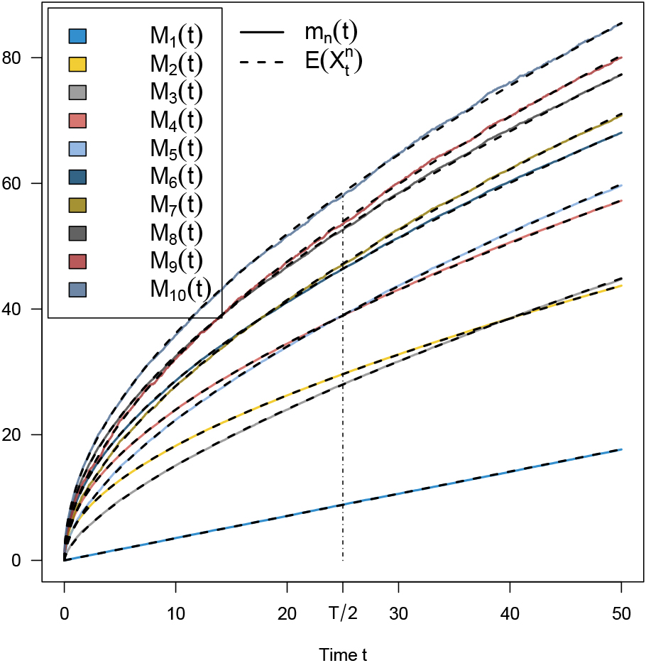
$\displaystyle M_{n}(t)\lx@stackrel{{\scriptstyle\Delta}}{{=}}\sqrt[n]{m_{n}(t)% }=\sqrt[n]{\mathbb{E}(X_{t}^{n})}$

(case $g(t)=at+b$ : linear time-dependent function).

We consider the following SDE as a numerical example to compute its moments, with: $\alpha=-2$ , $\beta=1$ , $\gamma=4$ , $g(t)=4t+35$ and $k=0$ (where: $g^{(0)}(t)\neq 0$ for all $t\geqslant 0$ ). We have:

$\displaystyle\left\{\begin{array}[]{l}dX_{t}=\left(-{\displaystyle\frac{8}{4t+% 35}}X_{t}+(4t+35)^{-2}\right)dt+4(4t+35)^{-2}dW_{t}\\ X_{0}=0,t\in[0,50]\end{array}\right.$ (8)

as an illustration, in this example we will use the formula from Theorem 3 (we can also use Theorem 1 and 2 we will find the same results). From the Eq. (7) we have:

$\displaystyle\mathbb{E}(X_{t}^{n})=\left\{\begin{array}[]{ll}0&\text{if }t=0\\ \frac{(4t+35)^{-2n}}{2\sqrt{\pi}}\sum_{j=0}^{n}\binom{n}{j}(1+(-1)^{j})\Gamma% \left(\frac{1+j}{2}\right)2^{\frac{5j}{2}}t^{n-\frac{j}{2}}&\text{if }t>0\end{% array}\right.$

In Fig. 1 we provide a visual comparison of the accuracy of the Monte-Carlo simulation approach (continuous lines) to the exact values (dashed lines) of the moments from $M_{1}(t)$ to $M_{10}(t)$ over time $t\in[0,50]$ .

Figure 1.

$1^{\text{st}}-10^{\text{th}}$ approximate and exact moments of Eq. (8), with: $\alpha=-2$ , $\beta=1$ , $\gamma=4$ , $g(t)=4t+35$ and $k=0$ .

(case $g(t)=\ln(t-T)$ : nonlinear time-dependent function).

We consider the linear non-homogeneous SDE, with: $\alpha=-1$ , $\beta=0$ , $\gamma=1/20$ and $g^{(k)}(t)$ :

$\displaystyle{g^{(k)}(t)}=\left\{\begin{array}[]{ll}\ln(t-50)&\text{if }k=0\\ (-1)^{k-1}{\displaystyle\frac{\Gamma(k)}{(t-50)^{k}}}&\text{if }k=1,2,3,\dots% \end{array}\right.$

for any $k\in\mathbb{Z}^{+}$ , we obtain Brownian bridge process:

$\displaystyle\left\{\begin{array}[]{l}dX_{t}={\displaystyle\frac{k}{t-50}}X_{t% }dt+{\displaystyle\frac{(t-50)^{k}}{20(-1)^{k-1}\Gamma(k)}}dW_{t}\\ X_{0}=20,t\in[0,50]\end{array}\right.$ (9)

From the Eq. (5), the exact high-order moments of Eq. (9) are given by:

$\displaystyle\mathbb{E}(X_{t}^{n})=\left\{\begin{array}[]{ll}20^{n}&\text{if }% t=0\\ 2^{-\frac{5n}{2}}\left(\frac{\mathrm{i}(t-50)^{k}}{5(-1)^{k}\Gamma(k)}\right)^% {n}\text{H}_{n}\left(\frac{-200\mathrm{i}\Gamma(k)}{50^{k}}\sqrt{\frac{2}{t}}% \right)t^{\frac{n}{2}}&\text{if }t>0\end{array}\right.$

If we have difficulties in calculating $\mathbb{E}(X_{t}^{n})$ by the last equation, we can also use the alternative Eq. (7), and we will find explicitly the same results for all non-negative integer $n$ .

$\displaystyle\mathbb{E}(X_{t}^{n})=\left\{\begin{array}[]{ll}20^{n}&\text{if }% t=0\\ \frac{20^{n}\left(\frac{t}{50}-1\right)^{nk}}{2(-1)^{nk}\sqrt{\pi}}\sum_{j=0}^% {n}\binom{n}{j}(1+(-1)^{j})\Gamma\left(\frac{1+j}{2}\right)\left(-\frac{50^{k}% \sqrt{2}}{400\Gamma(k)}\right)^{j}t^{\frac{j}{2}}&\text{if }t>0\end{array}\right.$

to illustrate, for any $k\in\mathbb{Z}^{+}$ we obtain explicitly the first, second, and third moments of Eq. (9):

$\displaystyle\mathbb{E}(X_{t})=20(-1)^{-k}\left(\frac{t}{50}-1\right)^{k}$ $\displaystyle\mathbb{E}(X_{t}^{2})=20^{2}(-1)^{-2k}\left(\frac{t}{50}-1\right)% ^{2k}\left(1+\frac{50^{2k}}{20^{4}\Gamma(k)^{2}}t\right)$ $\displaystyle\mathbb{E}(X_{t}^{3})=20^{3}(-1)^{-3k}\left(\frac{t}{50}-1\right)% ^{3k}\left(1+3\frac{50^{2k}}{20^{4}\Gamma(k)^{2}}t\right)$

The Fig. 2 shows the moments of Eq. (9) from $M_{1}(t)$ to $M_{10}(t)$ , where there is an excellent agreement between the Monte-Carlo simulation (continuous lines) and that were calculated using the formula (dashed lines). In the top for $k=1$ is first derivative of $g(t)$ and for $k=2$ is second derivative of $g(t)$ at the bottom. As one can see, the rough and unsmooth curves (continuous lines) are caused by the approximation errors in the simulated sample pathways. However, the graph displays the smooth curves (dashed lines) as the Eqs (5) and (7) produces the exact values of the high-order moments of Eq. (9).

Figure 2.

$1^{\text{st}}-10^{\text{th}}$ approximate and exact moments of Eq. (9), with: $\alpha=-1$ , $\beta=0$ , $\gamma=1/16$ and $g(t)=\ln(t-50)$ . Left: $k=1$ , Right $k=2$ .

(case $g(t)$ multiple nonlinear time-dependent function).

In that last example, we suppose a more complex SDE with multiple nonlinear time-dependent drift and diffusion coefficients (hybrid SDE), with parameters: $\alpha=-1/2$ , $\beta=1/2$ and $\gamma=8$ . We assume that $g(t)$ is defined on two states as follows:

$\displaystyle g(t)=\left\{\begin{array}[]{ll}t^{2}&\text{if }t\leqslant\frac{T% }{2}\\ {\displaystyle\frac{t^{3}}{t+1}}&\text{if }t>\frac{T}{2}\end{array}\right.$

for $k=2$ , we have the second and third derivative of $g(t)$ :

$\displaystyle g^{(2)}(t)=\left\{\begin{array}[]{ll}2&\text{if }t\leqslant\frac% {T}{2}\\ {\displaystyle\frac{2t(t^{2}+3t+3)}{(t+1)^{3}}}&\text{if }t>\frac{T}{2}\end{% array}\right.\quad\text{and}\quad g^{(3)}(t)=\left\{\begin{array}[]{ll}0&\text% {if }t\leqslant\frac{T}{2}\\ {\displaystyle\frac{6}{(t+1)^{4}}}&\text{if }t>\frac{T}{2}\end{array}\right.$

hence we have the following model:

$\displaystyle\left\{\begin{array}[]{l}dX_{t}={\displaystyle\frac{1}{2}}\left(-% {\displaystyle\frac{g^{(3)}(t)}{g^{(2)}(t)}}X_{t}+{\displaystyle\frac{1}{\sqrt% {{g^{(2)}(t)}}}}\right)dt+{\displaystyle\frac{8}{\sqrt{{g^{(2)}(t)}}}}dW_{t}\\ X_{0}=0,t\in[0,50]\end{array}\right.$ (10)

Here, we will directly use the formula from Theorem 1 to explicitly find the high-order moments. For example, we obtain explicitly the first, second, and third moments of Eq. (10):

$\displaystyle\mathbb{E}(X_{t})=\frac{\sqrt{2}}{4}\left(t\mathbf{1}_{\left\{t% \leqslant\frac{T}{2}\right\}}+\sqrt{\frac{t(t+1)^{3}}{t^{2}+3t+3}}\mathbf{1}_{% \left\{t>\frac{T}{2}\right\}}\right)$ $\displaystyle\mathbb{E}(X_{t}^{2})=\frac{t+256}{8}\left(t\mathbf{1}_{\left\{t% \leqslant\frac{T}{2}\right\}}+\frac{(t+1)^{3}}{t^{2}+3t+3}\mathbf{1}_{\left\{t% >\frac{T}{2}\right\}}\right)$ $\displaystyle\mathbb{E}(X_{t}^{3})=\frac{\sqrt{2}t(t+768)}{32}\left(t\mathbf{1% }_{\left\{t\leqslant\frac{T}{2}\right\}}+\sqrt{\frac{(t+1)^{9}}{t(t^{2}+3t+3)^% {3}}}\mathbf{1}_{\left\{t>\frac{T}{2}\right\}}\right)$

The results obtained by the Monte-Carlo simulation and which were calculated by Eq. (5) are shown in Fig. 3.

Figure 3.

$1^{\text{st}}-10^{\text{th}}$ approximate and exact moments of Eq. (10), with: $\alpha=-1/2$ , $\beta=1/2$ , $\gamma=8$ , $k=2$ and $g(t)=t^{2}\mathbf{1}_{\left\{t\leqslant T/2\right\}}\linebreak+t^{3}/(t+1)% \mathbf{1}_{\left\{t>T/2\right\}}$ .

4. Conclusion

Statistical moments provide relevant information, for example the peak location and width of the stochastic transient are determined by the first and second moment. However, an explicit solution for the Fokker-Plank equation is unlikely. Therefore, it is necessary to adopt approximate solutions. The evaluation of high-order moments is therefore valuable, and we can obtain them quickly and explicitly by the formulas discussed in this article, as shown in the above examples. In this sense, the resulting procedures are highly effective techniques for validating the effectiveness of Monte-Carlo simulations in stochastic modeling when using the linear SDE with nonlinear time-dependent drift and diffusion coefficients.

Footnotes

Acknowledgments

The authors are thankful to the editor and the anonymous referees for their thorough review and highly appreciate the comments and suggestions which significantly contributed to increasing the quality of our article. The work described in this paper was supported by the project entitled: “Mathematical Methods and Tools for System Performance” under the number “C00L03UN110120230001”, within the framework “Projets de Recherche Formation-Universitaire (PRFU)”, University of Tamanghasset, Ministry for Higher Education and Scientific Research, Algeria.

Supplementary material

The R code can be found on GitHub at https://github.com/acguidoum/R-code-MAS-231435, so that readers can replicate the results.

References

Allen

(2007). Modeling with itô stochastic differential equations (1st ed., Vol. 22). Springer-Verlag. doi: 10.1007/978-1-4020-5953-7.

Bishwal

J.P.N.

(2008). Parameter estimation in stochastic differential equations (1st ed.). Springer Berlin, Heidelberg. doi: 10.1007/978-3-540-74448-1.

Bishwal

J.P.N.

(2012). Parameter estimation in stochastic volatility models (1st ed.). Springer Cham. doi: 10.1007/978-3-031-03861-7.

Guidoum

A.C.

, & Boukhetala

(2020). Performing parallel monte carlo and moment equations methods for itô and stratonovich stochastic differential systems: R package Sim.DiffProc. Journal of Statistical Software, 96(2), 1-82. doi: 10.18637/jss.v096.i02.

Henderson

, & Plaschko

(2006). Stochastic differential equations in science and engineering. World Scientific. doi: 10.1142/5806.

Klebaner

F.C.

(2005). Introduction to stochastic calculus with applications (2nd ed.). Imperial College Press. doi: 10.1142/p386

Mackevicius

(2016). Stochastic models of financial mathematics (1st ed.). Elsevier. doi: 10.1016/c2016-0-01246-9.

Merton

R.C.

(1973). Theory of rational option pricing. The Bell Journal of Economics and Management Science, 4(1), 141-183. doi: 10.2307/3003143.

Øksendal

(2003). Stochastic differential equations: An introduction with applications (6th ed.). Springer Berlin, Heidelberg. doi: 10.1007/978-3-642-14394-6.

10.

Olver

F.W.

Lozier

D.W.

Boisvert

R.F.

, & Clark

C.W.

(2010). Nist handbook of mathematical functions (1st ed.). New York, United States: Cambridge University Press.

11.

R Core Team. (2023). R: A language and environment for statistical computing [Computer software manual]. Vienna, Austria. Retrieved from https://www.R-project.org/.

12.

Risken

(1996). The fokker-planck equation: Methods of solution and applications (2nd ed., Vol. 18). Springer-Verlag. doi: 10.1007/978-3-642-61544-3.

13.

Vasicek

(1977). An equilibrium characterization of the term structure. Journal of Financial Economics, 5(2), 177-188. doi: 10.1016/0304-405X(77)90016-2.

14.

Willink

(2005). Normal moments and hermite polynomials. Statistics & Probability Letters, 73(3), 271-275. doi: 10.1016/j.spl.2005.03.015.

Exact higher-order moments for linear non-homogeneous stochastic differential equation

Abstract

Keywords

1. Introduction

.

Proof..

.

Proof..

.

Proof..

(case g ⁢ ( t ) = a ⁢ t + b : linear time-dependent function).

(case g ⁢ ( t ) = ln ⁡ ( t - T ) : nonlinear time-dependent function).

(case g ⁢ ( t ) multiple nonlinear time-dependent function).

Footnotes

Acknowledgments

Supplementary material

References

(case $g(t)=at+b$ : linear time-dependent function).

(case $g(t)=\ln(t-T)$ : nonlinear time-dependent function).

(case $g(t)$ multiple nonlinear time-dependent function).