
Abstract
Stochastic volatility models have proven relevant for various purposes, e.g. explaining the term structure of implied volatility or correlations in absolute returns. When used in conjunction with jump models, they provide powerful tools that have been applied successfully in recent years. Volatility is however but one aspect of risk: in the frame of jump processes, the (local) intensity of jumps is another one, which is equally important. It thus seems natural to supplement stochastic volatility models with “stochastic jump intensity” ones, where the local intensity of jumps evolves according to a random dynamics. The aim of this preliminary work is merely to set up such models as extensions of the celebrated CGMY process, leaving their exploration both for risk management and for option pricing to further studies.
Background and motivation
Increment-stationary stochastic processes are typically unable to account for certain important features of financial markets, such as reproducing empirical Values at Risk (VaR) or implied volatility patterns. Introducing non stationarity requires to specify how the characteristic parameters of the models evolve in time in a way that is simple enough so as to lead to tractable subsequent treatment. Arguably the most popular ways to do so are through the use of a time-varying volatility. Two major classes of such models are stochastic volatility [13] and local volatility [6] ones. In the Gaussian and jump-diffusion frames, this amounts to replacing the instantaneous variance either by a stochastic process or by a function of the asset. In pure jump processes such as the CGMY model [4], this translates into letting the scale parameter C evolve. Quoting [4]: “For example, if one were to construct a model with a stochastic aggregate activity rate, then one could model C as an independent positive process, possibly following a square root law of its own”.
However, since the main feature of CGMY and similar processes is a fine modelling of jumps, and since it is precisely by taking into account jumps that these models improve upon diffusion ones, one may wonder why the parameter responsible for the jump intensity should be considered constant, while C would be allowed to vary. Indeed, contrarily to volatility, no local or stochastic jump intensity models have been put to use in financial engineering. A desirable extension of, say, CGMY should let all parameters evolve in time, and in particular the Y parameter, that finely tunes the jumps. Analogously to stochastic volatility and local volatility models, one should then design “stochastic jump exponent” and “local jump exponent” models.
A technical reason why models with varying jump intensity have not been widely considered so far is that their very definition is more challenging that, say, stochastic volatility ones. An operational reason is that, when it comes to risk control, the central notion considered in the literature is volatility, typically understood as a measure of variance, and this is why a huge number of models have been proposed that allow practitioners to finely tune it.
While volatility is obviously a central source of risk, it is not the only one. It has long been recognized that jumps occur in most financial logs [2,5] and that they also contribute to risk. Models with increasing precisions taking this aspect into account have been studied.
Our long-term program is to develop and study stochastic processes allowing one to model all dimensions of risk in a non-stationary way. The present article is a modest first step in this direction. We first recall in Section 2 some empirical studies from [7] showing (a) that the parameters
We then present some preliminary steps towards the design of operational models with varying jump intensity in Section 3, in the hope that they will foster subsequent studies. We will base our developments on tempered versions of so-called multistable motions and consider various extensions. Multistable motions [8,11,19,20] are generalization of Lévy motions where the jump intensity is allowed to vary in time in an exogenous manner. Tempered multistable motions were introduced in [7,12] and further studied in [17] where they are shown to be semimartingales and where the series representations of their field-based and independent increments asymmetrical forms are derived. See also [21] for a related process. In order to provide useful models in finance and other fields, one needs to specify the time evolution of jump intensity. In that view, we consider analogues of various stochastic volatility models in Section 4.
Numerical evidences
Numerical evidences of non-stationarity
We analyse in this section a log of the S&P 500, and estimate the functional parameters
S&P 500 data between 01/03/2002 and 01/02/2012 are shown on Fig. 1. Figure 2 displays the instantaneous
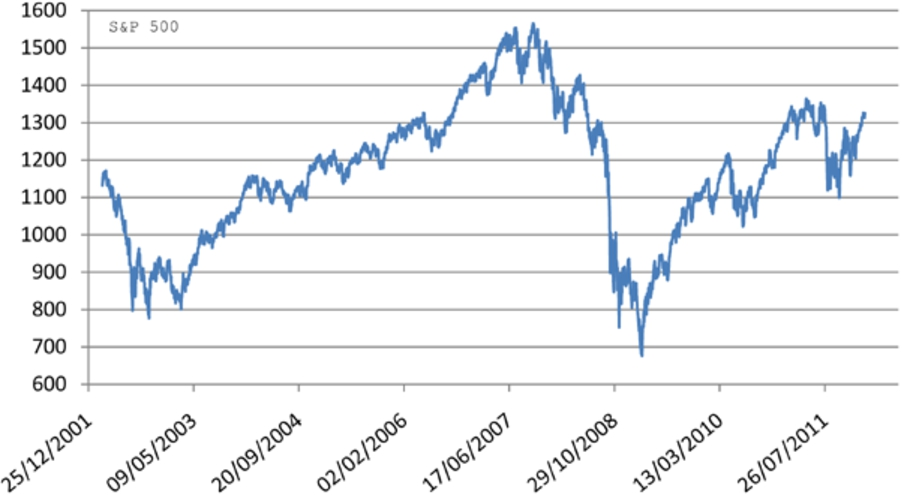
S&P 500 index between 01/03/2002 and 01/02/2012.
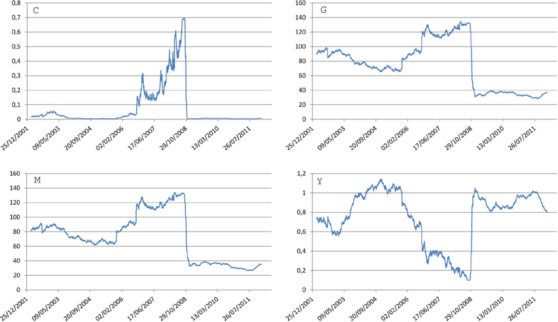
Evolution of C (top left), G (top right), M (bottom left) and Y (bottom right) for the S&P 500 index between 01/01/2002 and 31/12/2012.
As one can see it from the graphs, all parameters do vary significantly through time. Several interesting information may be drawn from those figures:
Except for the 2008–2009 crisis, movements on the parameters cannot be easily deduced from ones of the index log: the time evolution of the parameters reveal information that is concealed on the price variation.
Relative variations of the parameters are very large, with C ranging in
Consistent patterns appear: most notably, an increase in C always corresponds to a decrease in Y, while
The graphs may be roughly split into three zones (this is specially apparent from the evolution of C): from 01/03/2002 to 01/09/2006, characterized by small values of C, moderate values of G and M, and large values of Y; from 02/09/2006 to 01/12/2008, where C reaches large values, as do G and M, while Y drops to small ones; and finally from 02/12/2008 to 01/02/2012, where
Since the three zones mentioned in item 4 are notably different and each one is more or less homogeneous, it seems relevant to analyse them separately. Global estimates for the three zones are as follows:
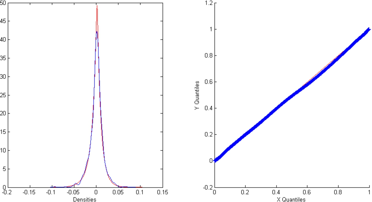
To assess the goodness of fit, comparisons between historical data and globally fitted CGMY models for each of the three zones are displayed through densities and QQ plots on Figs 3 to Fig. 5.
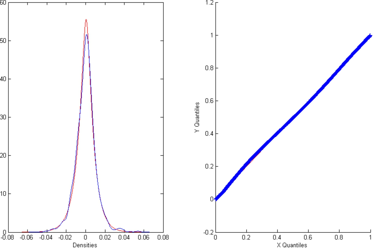
Densities (left) and QQ plots for zone 1; curve with lowest peak: historical data; curve with highest peak: CGMY model.

Densities (left) and QQ plots for zone 2; curve with lowest peak: historical data; curve with highest peak: CGMY model.
Densities (left) and QQ plots for zone 3; curve with lowest peak: historical data; curve with highest peak: CGMY model.
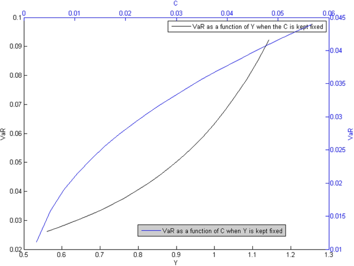
VaR as a function of Y (bottom curve) and C (top curve), when all other parameters are kept constant, region 1.
Characterizing the impact on VaR of the various parameters in the CGMY model is a complex issue: it depends on the confidence threshold and on a complex interplay between the values of the parameters. For instance, it would seem intuitive that decreasing Y should increase VaR. However this is only the case when the threshold is in a certain range, which in turn depends on the values of the other parameters. Since VaR measures extreme events, one might think of using the asymptotic formulas (7.6) and (7.7) of [3] (see also [18]). However, for typical parameters values observed on markets, and at the threshold of, say,
The aim of this section is to provide graphical illustrations of how changes of C and Y impact VaR, and to compare the influences of these two parameters. Indeed, Section 2.1 suggests that both C and Y do vary in time. A natural question is then whether such variations have a significant impact on VaR, or if they may be safely ignored. In order to elucidate this point, we shall make use of the empirical results of the previous section to set the ranges of variation of the parameters. It occurs that using the whole ranges between 01/01/2002 and 31/12/2012 results in unrealistically large variations of VaR. For this reason, we will rather work with the three roughly homogeneous zones identified above.
We draw two kinds of graphs;
VaR as a function of C when Y is kept constant, and as a function of Y when C is kept constant. The value of the parameter which is kept constant is set to the one estimated globally on the considered region. The varying parameter spans the range of the local estimates in the region. This is on Figs 6 to 8.
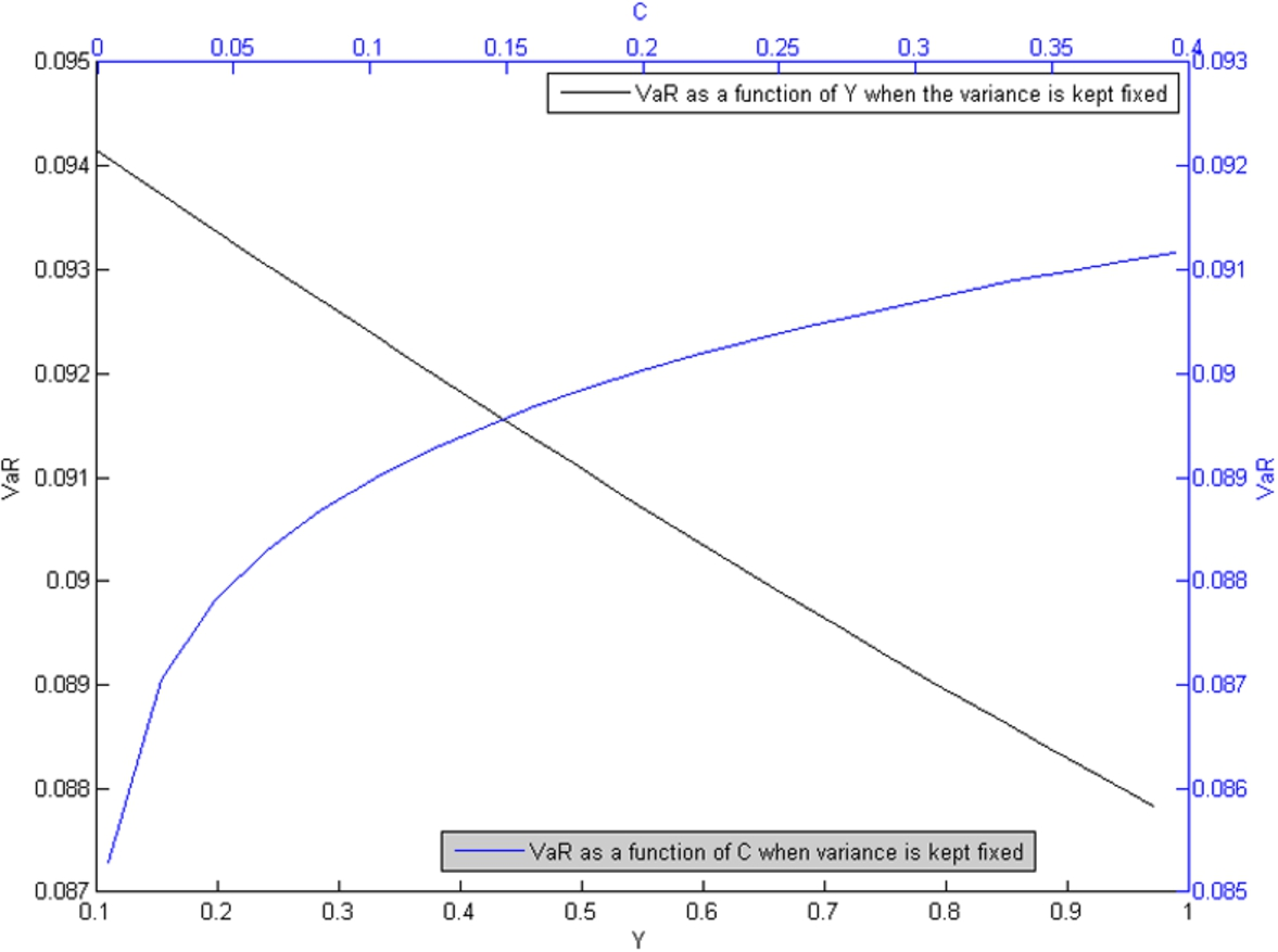
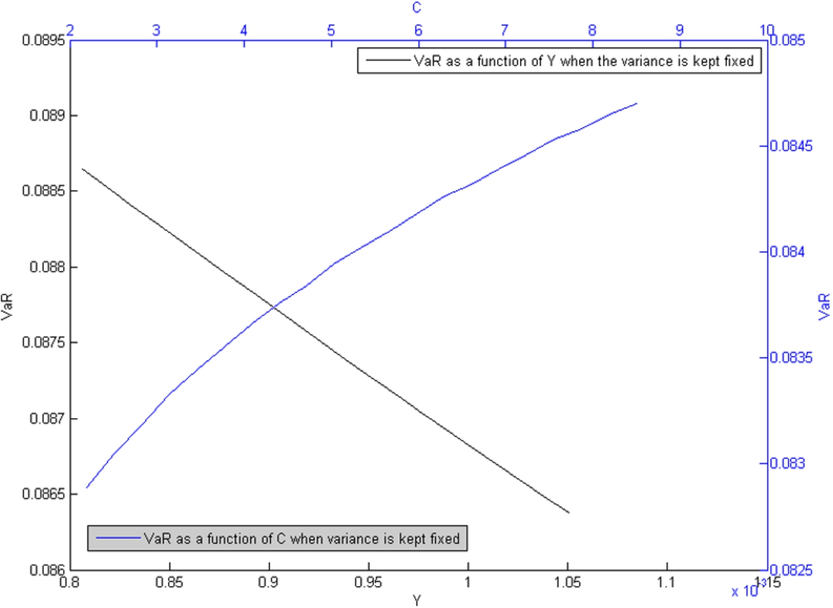
VaR either as a function of C when the variance is kept constant or as a function of Y when the variance is kept constant: recall that the variance of a CGMY process is equal to
We display two more graphs: Fig. 12 plots the evolution of C as a function of Y that yields a constant VaR (the bounds on Y are the ones of region 2): this is intended to stress the fact that a given fixed VaR may be obtained with significantly different levels of global activity C when Y varies in a realistic range. Figure 13 shows how the variance evolves when C spans its range of local estimates in region 1 and Y is adjusted accordingly so as to keep the VaR constant (equal to the one estimated with the global parameters in region 1). This is to emphasize that the instantaneous variance alone is not sufficient to characterize VaR: here, the same VaR is obtained with a variance undergoing a variation of 40%.
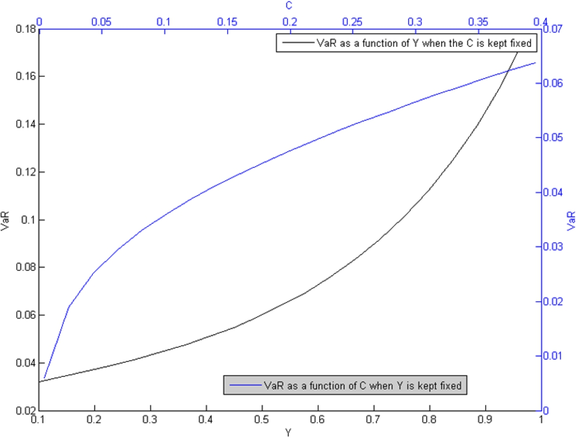
VaR as a function of Y (bottom curve) and C (top curve), when all other parameters are kept constant, region 2.
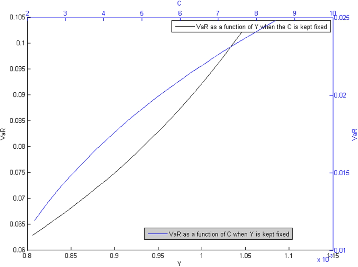
VaR as a function of Y (bottom curve) and C (top curve), when all other parameters are kept constant, region 3.
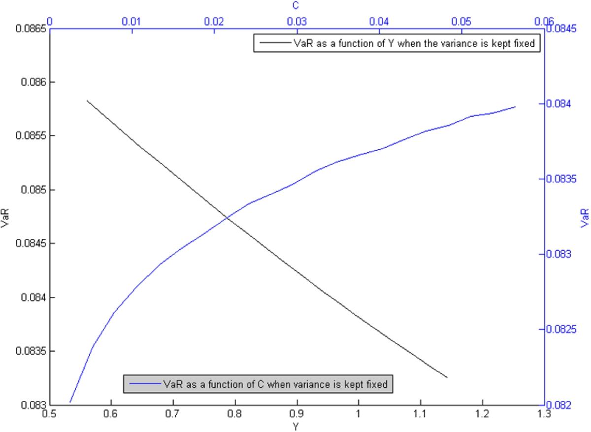
VaR as a function of Y (decreasing curve) and C (increasing curve), when the variance is kept constant, region 1.
VaR as a function of Y (decreasing curve) and C (increasing curve), when the variance is kept constant, region 2.
VaR as a function of Y (decreasing curve) and C (increasing curve), when the variance is kept constant, region 3.
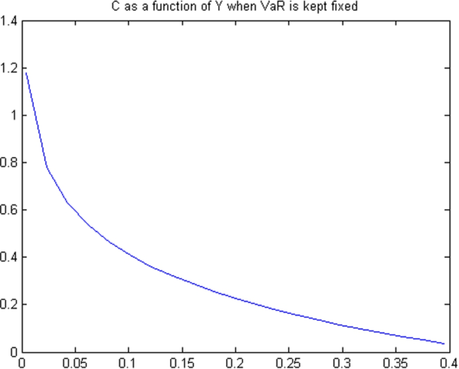
C as a function of Y that yields a constant VaR (bounds of region 2).
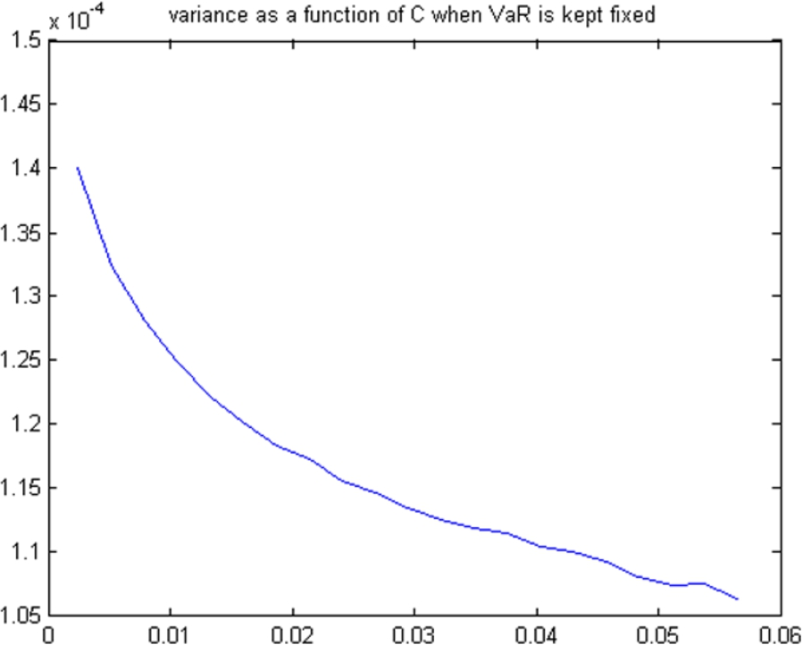
Variance as a function of C, where Y is adjusted so that VaR remains constant (bounds of region 1).
In this section, we give two constructions of tempered multistable processes and their generalization to the case of a random jump intensity.
Construction through characteristic function
Fix parameters
The density of the associated Lévy measure reads:
Campbell formula allows us to compute the characteristic function of the random variable
In the general case, we need to compensate the Poisson measure. The compensated measure
Let φ be a measurable function on
Note that
The process
Let us now move to the case of real interest to us, that is, assume now that Y is an element of
We construct the CGMY process with stochastic jump exponent as the mixture characterized by the following measure on
For this definition to make sense, we need to verify that
Series representation
A CGMY process is a tempered stable process in the sense of [22] with (we use the notations of [22]):
The first four series are the ones considered in [22], pages 696 and 701. As for the last one, it is obtained as follows: [22] on page 696 introduces a sequence of i.i.d. r.v.
The value of
Representation (3) allows us to define two versions of multistable tempered processes as follows:
Let
The field-based tempered multistable process parametrized by
The independent-increment tempered multistable process parametrized by
Remark that we do not make any assumption of regularity on
The proof that the series above converge almost surely is a straightforward extension of the ones in [22]. □
The generalization to the case of random jump exponent is then straightforward:
Let
The field-based tempered multistable process with random jump exponent parametrized by Υ is the random process
The independent-increment tempered multistable process with random jump exponent parametrized by Υ is the random process
Remark that we do not require independence between Υ and Z in these definitions. This will be however needed in applications to avoid technical complications.
In order to explore the benefit of using models with a time-varying local jump exponent in financial applications, the basic idea is to consider stochastic time evolutions of the form:
For such models to be practical and amenable e.g. to option pricing or risk management, it is necessary to specify the evolution of Y. In a roughly similar way to local and stochastic volatility models, there are two ways to do so. The first one consists in defining “self-stabilizing” processes, where the evolution of Y depends on the value of the process. This path is explored in [9,10]. In this work we deal with the second possibility: we specify the evolution of Y through a separate stochastic differential equation, defining “stochastic local jump exponent” models, much in the spirit of stochastic volatility models. Our aim here is merely to propose reasonable models, leaving their theoretical as well as experimental study for further work.
General frame
The general idea is to let Y be a continuous ergodic Markov process ranging in a real interval I, independent of the variables
Let us start with a property related to the martingale character in the independent increments case:
The process
The proof of this result is standard if we assume Υ deterministic. In the random case, it follows from the independence between the random variables that govern the jumps of
Our first model mimics the Hull and White model where we have substituted Y for the volatility, and replaced the Wiener driving noise of the spot price by a tempered multistable one. It reads as follows:
A tempered multistable motion with random local jump exponent, Heston variant
The second model mimics the Heston model where we have substituted Y for the volatility, and replaced the Wiener driving noise of the spot price by a multistable one.
Since Y appears as an exponent in the definition of multistable processes, it may seem more relevant to model the evolution of its logarithm, leading to
Figures 14 and 15 display realizations of these two variants sampled on one thousand points, with
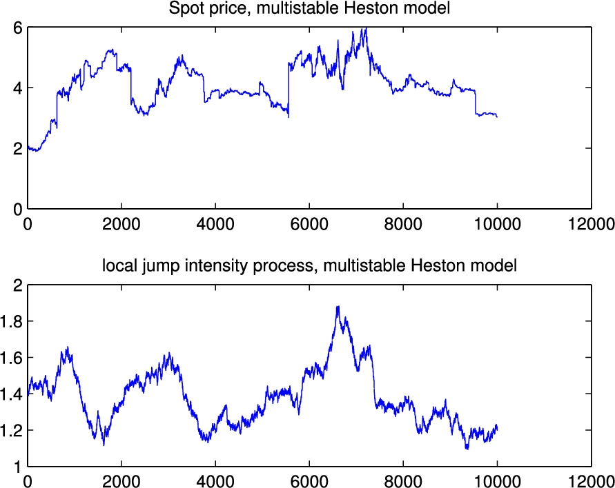
Spot price and local jump intensity process for model (11).
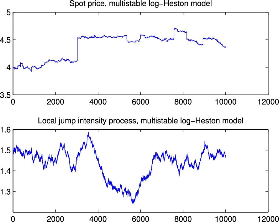
Spot price and local jump intensity process for model (12).
Footnotes
Acknowledgements
J. Lévy Véhel gratefully acknowledges support from SMA Group as well as many fruitful discussions with P. Desurmont, O. Le Courtois, M. Majri, H. Rodarie and C. Walter.