Synthetic Minority Over-sampling Technique (SMOTE) for handling imbalanced data in poverty classification

Abstract

Poverty data in official statistics data is important for development planning. The lower percentage of the poor recorded yearly indicates good development of a country. Moreover, there is always a problem when performing an inferential and classification analysis because of the imbalanced data, thereby leading to biases in the estimation results and prediction errors in the classification. One of the solutions to this problem is using Synthetic Minority Over-sampling Technique (SMOTE). Therefore, this study aims to evaluate the inference and classification quality using the binary logistic regression model without and with SMOTE. The data utilized was the poverty status of households in the rural and urban areas in East Java, Indonesia as contained in the 2019 National Socio-Economic Survey. Furthermore, the variables used are poverty status of the household, the age of the household head (HH), the ratio of household members who are employed, gender of the HH, number of household members, education level of HH, and occupation of the HH. It was concluded that the model with SMOTE approach was better at inference and classifying the results.

Keywords

Poverty inference evaluation classification evaluation SMOTE binary logistic regressions

1. Introduction

Poverty data in official statistical data is important for development planning. This is the reason poverty alleviation was rated first in the Sustainable Development Goals, which states “end poverty in all its forms everywhere” [1]. The poverty rate in Indonesia has been experiencing a downward trend yearly, thereby showing good indicators. However, it has been observed from the distribution that the majority of the poor in this country are on Java Island, reaching 12.48 million people, and representing 50.7% of the poor nationally. Among the provinces on Java Island, East Java has the highest number of poor people, thereby causing the place to be poverty enclaved according to the criteria of the National Team for the Acceleration of Poverty Reduction (TNP2K).

Poverty data in Indonesia is obtained rawly from National Socio-Economic Survey (SUSENAS), indicating the possibility of obtaining an imbalanced data composition. For example, the results of SUSENAS showed that the poverty rate in East Java reached 10.37%, while in Indonesia reached 9.41% meaning that it is imbalanced. Imbalanced data often cause problems in the classification method, such as biases in the estimation result and increased prediction errors in the classification, particularly in the minority class [2]. Furthermore, it is likely to cause the resulting standard error to be overestimated, and in the case of the classification model, it is likely to cause overfitting.

There are two approaches to overcome the imbalanced data problem, namely solutions at the data level or the algorithm level. The data-level solution is proposed by balancing the distribution of the majority and minority classes using under-sampling, over-sampling, or a combination of both methods. Meanwhile, that of algorithm level is conducted by adjusting the system without changing the data distribution using the cost function, modifying the classification method, or ensemble [2]. It is accomplished by adding weights to the sample, according to [3], but this method was unable to classify the accuracy satisfactorily compared to the over-sampling approach. It has been observed that the data-level solution has advantages over the algorithm-level in terms of flexibility when choosing the classification method used [4]. For example, the data-level solutions are applicable in several classification methods, but that of the algorithm is only utilized for specifics. It is important to note that the over-sampling is more widely used than the under-sampling method. This is because the under-sampling eliminates data in the majority class, thereby causing important information to be lost [2]. An example of the over-sampling method that is often used is Random Over-sampling (ROS), but it usually causes overfitting of the model [5]. Consequently, several over-sampling techniques for solving this problem have been developed, and the most widely used was the Synthetic Minority Over-sampling Technique (SMOTE) [6]. This method deals with generating new or artificial data randomly along the line between the data in the minority class and its nearest neighbor.

Several logistic regression studies have been performed using SMOTE to handle data imbalances and the results showed that it was able to improve the quality of classification. In [7], SMOTE’s application in logistic regression improved the classification of minor classes compared to those without SMOTE. Another study conducted by [8] showed that the application of SMOTE was able to improve classification accuracy in minor classes and was able to overcome overfitting in the model.

It has been observed that poverty classification in Indonesia, especially in East Java Province, has been conducted generally without considering imbalanced data on household poverty status. For example, the classification of household poverty by [9, 10] showed that the proportion of imbalanced data had not been considered. Also, the study [11] on household poverty in rural and urban areas does not consider the unbalanced proportion of data. The observation from previous studies showed that the model quality inference using SMOTE is still less explored. Therefore, this study aims to fill the gap by:

Evaluating the inference quality of the logistic regression model for rural and urban household poverty in East Java Province using binary logistic regression without and with SMOTE.

Evaluating the quality of binary logistic regression classification without and with SMOTE.

In Section 2, the methodology of this study explains the data and variables used. The explanation of SMOTE and logistic regression will be presented in this section. Then, the descriptive analysis, inferential analysis, and classification evaluation will be presented in Section 3. Finally, the conclusion will be generated in Section 4.

2. Methodology

Table 1
Variable used and its categories

Variable notation	Variable description	Categories
Y	Household poverty status	1 $=$ Poor
		0 $=$ Non Poor ${}^{*}$
X1	The age of the household head (HH)	Continuous variable
X2	The ratio of the number of working household members	Continuous variable
D31	Gender of the household head	1 $=$ Female
		0 $=$ Male ${}^{*}$
D41	Number of the household members	1 $=$ $>$ 4
		0 $=$ 1–4 ${}^{*}$
D51	Education level of the household head	1 $=$ Middle school and lower
		0 $=$ High school and higher ${}^{*}$
D61	Occupation of the household	1 $=$ Did not work
D62		2 $=$ Agriculture
		0 $=$ Non agriculture ${}^{*}$

${}^{*}$ Reference categories.

This study uses the March 2019 SUSENAS data where the household is the sampling unit. The total sample for the March 2019 SUSENAS for East Java province is 30,021 households, consisting of 15,800 households in urban areas and 14,221 in rural areas. A descriptive-analytical method was used through cross-tabulation, while inferential analysis and classification evaluation was performed using binary logistic regression without and with SMOTE methods. The imbalanced data problem was mitigated using the SMOTE method by finding the nearest neighbors within the minority class. The dependent variable was the poverty status of households, which are categorized into poor and non-poor, while the independent variables are the age of the household head (HH), the ratio of the number of employed household members, the HH gender, number of the household members, the HH education level, and the HH’s occupation. Table 1 shows the variables utilized and their categories.

3. SMOTE and Logistic regression

3.1 SMOTE

The SMOTE method was developed by Chawla et al. [6] to solve the imbalanced data problems. This method differs from the previously proposed oversampling methods. The reason being that those oversampling methods deal with multiplying random observations, while the SMOTE reproduces artificial data in classes, in which the lesser or minor class is equalized to the major ones. Furthermore, the artificial or synthesis data was generated based on the k-nearest neighbor, which is determined by considering the ease of implementation. Generating artificial data is different for data with a numerical scale versus data with a categorical scale. The numerical data were measured using Euclidean distance, while categorical data was simpler, namely the mode value. The distance between minor classes and categorical scale variables was calculated using the Value Difference Metric (VDM) formula [12] as follows:

$\displaystyle\Delta(X,Y)=w_{x}w_{y}\sum_{i=1}^{N}\delta(x_{i},y_{i})^{r}$ (1)

Where $\Delta(X,Y)$ is the observed distance of $X$ and $Y$ , $N$ indicates the number of the independent variable, $w_{x}w_{y}$ are negligible observation weights, $r$ is 1 for Manhattan distance and 2 is for Euclidean distance, while $\delta(x_{i},y_{i})$ is the categorical distance.

$\displaystyle\delta(x_{i},y_{i})=\sum_{i=1}^{n}\left|\frac{C_{1i}}{C_{1}}-% \frac{C_{2i}}{C_{2}}\right|^{k}$ (2)

Where $\delta(x_{i},y_{i})$ is the distance of $x$ and $y$ , $C_{1i}$ and $C_{2i}$ are the number of times vector 1 (classify into category non-poor household) and 2 (classify into category poor household), respectively, $C_{1}$ and $C_{2}$ are the total number of times values 1 and 2 occurred, respectively, $n$ is the number of categories, while $k$ is constant, which is usually 1.

The procedures for generating artificial data include:

Numerical Data

Calculate the difference between the main vector and its k-nearest neighbors.

Multiply the difference by the random number between 0 and 1.

Add this difference to the principal value of the original vector to obtain a new principal vector.

Categorical Data

Select the main vector and its k-nearest neighbors among the ones considered for the face value. Then select randomly when the values are the same.

Create a value from the newly created class example data.

3.2 Logistic regression

The logistic regression analysis determines the relationship between responses and one or more explanatory variables. In binary logistic regression, the dependent variable is divided into two categories, such as the event of success denoted as $Y=$ 1 and the event of failure represented as $Y=0$ [13]. This logistic regression model with $p$ independent variables is generally written as follows.

$\displaystyle\pi(x)=\frac{\exp(\beta_{0}+\beta_{1}x_{1}+\ldots+\beta_{p}x_{p})% }{1+\exp(\beta_{0}+\beta_{1}x_{1}+\ldots+\beta_{p}x_{p})}$ (3)

The logit transformation is then performed as follows:

$\displaystyle g(x)=\beta_{0}+\beta_{1}x_{1}+\beta_{2}x_{2}+\ldots+\beta_{p}x_{p}$ (4)

The Maximum Likelihood Estimator (MLE) method was used for the parameter estimation in logistic regression and its procedure includes maximizing the likelihood function to obtain the observed data set. The first step in applying this method was to form the likelihood function as follows:

$\displaystyle l(\beta)=\prod_{i=1}^{n}\left[(\pi(x_{i}))^{y_{i}}[1-\pi(x_{i})]% ^{1-y_{i}}\right.$ (5)

It is important to note that the maximum likelihood method’s principle deals with maximizing the logarithm of the probability function:

$\displaystyle L(\beta)=\ln[l(\beta)]$ (6)

Table 2

Poverty status according to each variable

		Status of residual area
Variable	Categories	Rural		Urban
		Poor	Non poor	Poor	Non poor
Gender of the HH	Female	10.57	89.43	4.29	95.71
	Male	8.97	91.03	3.68	96.32
Number of the household members	$>$ 4	15.72	84.28	7.45	92.55
	1–4	7.43	92.57	2.72	97.28
Education of the HH	Middle School and lower	10.20	89.80	5.20	94.80
	High School and higher	3.38	96.62	1.38	98.62
Occupation of the HH	Did not work	13.18	86.82	5.52	94.48
	Agriculture	11.35	88.65	7.19	92.81
	Non Agriculture	7.00	93.00	2.93	97.07

Source: SUSENAS 2019 (processed).

Obtaining an estimate of the logistic regression coefficient ( $\hat{\beta}$ ) was conducted by decreasing $L(\beta)$ and equating it to zero. Therefore, the likelihood equation was expressed as follows:

$\displaystyle\frac{\partial L(\beta)}{\partial(\beta)}=\sum_{i=1}^{n}x_{i}[y_{% i}-\pi(x_{i})]=0$ (7)

Equation (7) is non-linear with respect to $\beta$ according to [13], therefore, special methods such as complex iterations with computerization are needed to determine the value of $\hat{\beta}$ .

3.3 The goodness of fit

The model suitability test, also known as the Goodness of Fit, refers to a test for determining whether the obtained model is appropriate/fit to analyze the dependent variable. An example of the method for measuring the Goodness of fit is the classification table [13], which involves the comparison of sizes to get the best model. The classification measures used in this study include accuracy, sensitivity, specificity, g-means, and AUC [14, 15, 16]. G-mean is defined as geometric mean of sensitivity and specificity.

$\displaystyle\text{G-means}=\sqrt{\textit{Sensitivity}\times\textit{% Specificity}}$ (8)

4. Result and discussion

4.1 Descriptive analysis

It has been observed that the poor households percentage in rural areas was higher than that of urban in East Java Province. According to the March 2019 SUSENAS, the percentage of poor households in rural areas was 12.9%, while that of urban was 6.3%. Table 2 shows the percentages of poor households based on each independent variable.

It was observed that the percentage of female-headed households with poor status was higher than males in both rural and urban areas. The female head of household (HH) had limitations in getting a job, particularly those requiring physical strength, this probably caused most of them to be unemployed. Specifically, 29% and 37.1% of female household heads are unemployed in rural and urban areas, respectively. Furthermore, the majority of HH had not completed the government’s 12-year compulsory education program. In rural and urban areas, only 13.9 and 36.7% have a high school education, respectively thereby causing households to have a higher tendency to be poor in both areas. According to [17], the rural poor had junior high school education and below, while the urban poor had higher education. This is because there was higher competition for jobs in the urban area, which led to several highly educated people not getting jobs. This is reflected in the high percentage of household heads with high school education and above who do not work in urban areas. It was therefore concluded that the percentage of household heads with high school education and above who are not working in urban areas was higher compared to the rural.

A different pattern was observed between rural and urban areas in terms of HH employment variable. In rural areas, poor households had the highest percentage when the heads were not working, but most of these individuals worked in the agricultural sector in the urban. The study by [18] showed that household heads who are unemployed have a significant effect on household poverty.

Table 3
Comparison model with and without SMOTE

Variable	$\hat{\beta}$	Standard error	$P$ -value	$\hat{\beta}$	Standard error	$P$ -value	$\hat{\beta}$	Standard error	$P$ -value	$\hat{\beta}$	Standard error	$P$ -value
	Rural						Urban
	Without SMOTE			SMOTE			Without SMOTE			SMOTE
Intercept	$-$ 3.728	0.204	0.000 ${}^{***}$	$-$ 0.832	0.139	0.000 ${}^{***}$	$-$ 3.890	0.244	0.000 ${}^{***}$	$-$ 0.659	0.197	0.000 ${}^{***}$
X1	0.012	0.003	0.000 ${}^{***}$	0.013	0.002	0.000 ${}^{***}$	0.002	0.004	0.603	0.009	0.004	0.015 ${}^{**}$
X2	$-$ 1.073	0.154	0.000 ${}^{***}$	$-$ 1.345	0.126	0.000 ${}^{***}$	$-$ 1.769	0.235	0.000 ${}^{***}$	$-$ 2.262	0.197	0.000 ${}^{***}$
D31	0.176	0.096	0.066 ${}^{*}$	0.688	0.070	0.000 ${}^{***}$	0.070	0.139	0.612	0.379	0.019	0.000 ${}^{***}$
D41	0.713	0.077	0.000 ${}^{***}$	1.050	0.064	0.000 ${}^{***}$	1.000	0.105	0.000 ${}^{***}$	0.900	0.095	0.000 ${}^{***}$
D51	1.023	0.158	0.000 ${}^{***}$	0.162	0.085	0.0574 ${}^{*}$	1.205	0.146	0.000 ${}^{***}$	0.868	0.106	0.000 ${}^{***}$
D61	0.064	0.141	0.648	0.412	0.100	0.000 ${}^{***}$	0.020	0.167	0.904	0.018	0.128	0.889
D62	0.414	0.078	0.000 ${}^{***}$	0.413	0.063	0.000 ${}^{***}$	0.647	0.138	0.000 ${}^{***}$	0.977	0.124	0.000 ${}^{***}$

Source: SUSENAS 2019 (processed). ${}^{*}$ significant at $\alpha=$ 10%, ${}^{**}$ significant at $\alpha=$ 5% and ${}^{***}$ significant at $\alpha=$ 1%.

In the aspect of household members number, those having more than four people had a higher percentage of poor compared to when they are lesser, in both rural and urban areas. The poverty rate among rural households with more than four members was 15.72%, while those less than this number were 7.43%. In urban areas, the percentage of poor households with more than four members was 7.45%, while those with the fewer numbers were 2.72%. The high percentage of poor-status households with more members was caused by the lower per capita income/expenditure distributed among the individuals [19].

It is also important to note that as people become older, they tend to be more established because of the increase in experience and income. For example, the average age of the household heads in rural areas was 52–53 years but was 50–51 years in urban. In these two areas, poor household heads had a higher average age compared to those who were not poor. Specifically, the non-poor in rural areas were 52–53 years old, while the poor were 55–56.

Relying solely on the household head is sometimes not enough to meet household needs, rather the help of members is also needed. This means that when there is an increase in the number of employed household members, meeting needs becomes easier. It was also observed that the poor households in both rural and urban areas tend to have hackwork compared to those who are not poor.

4.2 Inferential analysis

A comparison of the modeling using logistic regression without and with SMOTE approach has been conducted. It was observed from Table 3 that out of the seven variables used, six have a significant effect on the status of poverty in rural areas, while that of urban areas was four. Furthermore, the standard error in the model without SMOTE tends to be overestimated. This standard error is an important component in estimating a parameter value as described by [20] that a small standard error refers to a better parameter estimation. The results showed that the models with SMOTE have a smaller standard error estimation but do not produce a larger difference in regression parameters estimated from the model without SMOTE. This improvement in the standard error estimation using SMOTE model led to an increase in the number of variables that have a significant effect on the poverty status of rural and urban areas since the resulting $p$ -value was smaller. It was concluded that the significant variables in rural and urban areas are the age of the household head, the ratio of working household members, gender of HH, HH engaging in agriculture, the number of household members, and the education of HH. In contrast, the unemployed HH were significant in rural areas but not in the urban.

The odds ratio results show that households with the less ratio of working household members, the older of HH, households with more than four household members, a female head of household, with lower than high school education, and those not working or working in the agricultural sector tend to be a poor household. These results are also in line with the descriptive analysis, where the characteristics of poor households are those with more than four household members, a female head of household, lower than high school education, and not working or working in the agricultural sector.

Table 4
The results of simultaneous parameter testing without and with SMOTE

Model	Without SMOTE	SMOTE
Rural	359.1	756.7
Urban	331.5	534.7

Source: SUSENAS 2019 (processed).

Table 5

Classification performance comparison

	Model	Sensitivity	Specifically	G-means	AUC
Without SMOTE	Rural	0	100%	0	0.6629
	Urban	0	100%	0	0.7341
SMOTE	Rural	67.77%	57.19%	0.6225	0.6795
	Urban	75.56%	60.99%	0.6788	0.7413

Figure 1.

Area Under ROC Curve for Urban Model (AUC without SMOTE 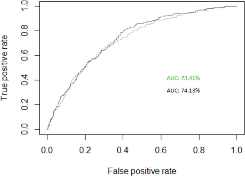$=$ 73.41%; and AUC with SMOTE $=$ 74.13%).

Table 4 shows that the simultaneous parameter testing using the Likelihood Ratio Test both with and without SMOTE produced consistent results, thereby causing $H_{0}$ to be rejected. All of the values of $G>\chi_{(0.10;8)}^{2}$ was 15.057, and the 10% significance level for both models showed that a minimum of one independent variable affected the poverty status of rural and urban households in East Java in 2019.

4.3 Classification evaluation

A classification comparison between the model with and without the SMOTE was performed. Table 5 shows that the accuracy value of the model without the SMOTE has high specificity in rural and urban areas. However, it has a sensitivity value of 0%, indicating that the model was unable to classify the category of poor households. The specificity value of 100 means that the model was able to correctly classify the category of non-poor households by 100%. This high specificity with zero value of sensitivity indicated overfitting, which often occurs due to the logistics curve leading to one category [21]. This condition caused the model to be unable to correctly predict new observations in one of the categories, namely poor. Furthermore, the value of g-means or geometric mean of sensitivity and specificity was zero, which indicated a poor classification performance. In other words, it means that there is an overfitting problem in the model [22].

Figure 2.

Area Under ROC Curve for Rural Model (AUC without SMOTE 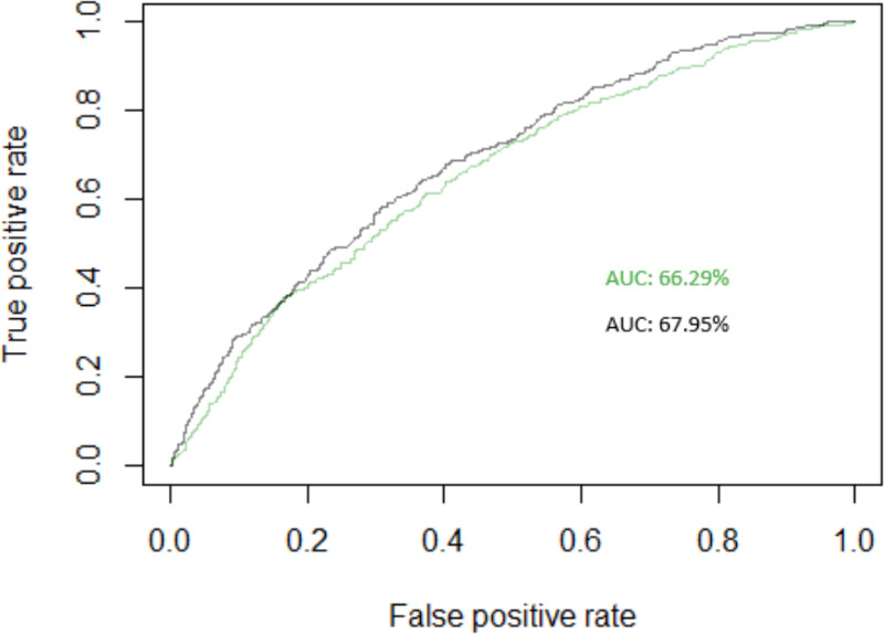$=$ 66.29%; and AUC with SMOTE $=$ 67.95%).

It was also observed that the model with the SMOTE produced a lower specificity than the model without the SMOTE approach, but had a higher sensitivity value. In the rural model with the SMOTE, the sensitivity value of 67.77 means that the model was able to correctly classify the poor households by 67.77%. Meanwhile, in the urban model, the sensitivity value was 75.56%, indicating that it was able to correctly classify the poor households by 75.56%. The model with the SMOTE approach has a higher g-means value than the model without SMOTE, which is consistent with [15] that SMOTE increased the g-means value in imbalanced data.

The model with SMOTE also had better performance based on the AUC value compared to the one without the SMOTE approach. The higher AUC value in the model with the SMOTE approach is in accordance with [22] discovering that the SMOTE produced a much higher AUC value than the other model. Also, the study by [7] found that as the AUC value increases or gets closer to one, the accuracy of the model becomes better. It is also showed by the area under the Receiver Operating Characteristic (ROC) curve in Fig. 1 for the urban model and Fig. 2 for the rural model, which is slightly wider in the model with SMOTE than without SMOTE. It is important to note that a good classification performance on imbalanced data was not only recognized from the accuracy value but from a good model with no overfitting problem [22]. Table 5 shows that the model with the SMOTE approach mitigate the problem of overfitting, indicating that it classified the poor households in rural and urban areas better than without SMOTE.

5. Conclusion

The logistic regression model of imbalanced data causes biased estimation results like overestimation of the standard error, as well as the model not being able to classify the minority category, such as the poor households. The SMOTE approach has been proven to overcome both inferential and classification quality problems. Meanwhile, the model without SMOTE produced more statistically significant variables with little differences in the regression coefficient estimated. It was concluded that the model with the SMOTE approach was better at classifying the poverty status of households in rural and urban areas in East Java Province.

References

Johnston

. Arsenic and the 2030 Agenda for sustainable development. Arsen Res Glob Sustain – Proc 6th Int Congr Arsen Environ AS 2016. 2016; pp. 12-4.

Santoso

Wijayanto

Notodiputro

Sartono

. A Comparative Study of Synthetic Over-sampling Method to Improve the Classification of Poor Households in Yogyakarta Province. IOP Conf Ser Earth Environ Sci. 2018; 187(1): 0-18.

Maalaouf

Siddiqi

. Robust Weighted Kernel Logistic Regression In Imbalanced And Rare Events Data. Orphanet J Rare Dis. 2009; 21(1): 1-9.

Ramentol

Caballero

Bello

Herrera

. SMOTE-RSB *: A hybrid preprocessing approach based on oversampling and undersampling for high imbalanced data-sets using SMOTE and rough sets theory. Knowl Inf Syst. 2012; 33(2): 245-65.

Tetko

Livingstone

Luik

. Neural Network Studies. 1. Comparison of Overfitting and Overtraining. J Chem Inf Comput Sci. 1995; 35(5): 826-33.

Chawla

Bowyer

Hall

Kegelmeyer

. SMOTE: Synthetic Minority Over-sampling Technique. J Artif Intelligance Res. 2002; 30(2): 321-57.

Barro

Sulvianti

Afendi

. Penerapan Synthetic Minority Oversampling Technique (Smote) Terhadap Data Tidak Seimbang Pada Pembuatan Model Komposisi Jamu. Xplore J Stat. 2013; 1(1).

Mujaddid

Adiwijaya Al-faraby

. Analisis Churn Prediction Menggunakan Metode Logistic Regression Dan Smote (Synthetic Minority Over-sampling Technique) Pada Perusahaan Telekomunikasi. eProceedings Eng. 2017; 4(3): 5046-54.

Annur

. Klasifikasi Masyarakat Miskin Menggunakan Metode Naive Bayes. Ilk J Ilm. 2018; 10(2): 160-5.

10.

Effendy

Purbandini

. Klasifikasi Rumah Tangga Miskin Menggunakan Ordinal Class Classifier. J Nas Teknol dan Sist Inf. 2018; 4(1): 30-6.

11.

Miftahuddin

. Analisa Karakteristik Rumah Tangga Miskin dengan Metode Regresi Logistik Terbaik. J Mat Stat Dan Komputasi. 2011; 7(2): 79-91.

12.

Cost

Salzberg

. A Weighted Nearest Neighbor Algorithm for Learning with Symbolic Features. Mach Learn. 1993; 10(1): 57-78.

13.

Hosmer

Lemeshow

. Applied Logistic Regression. 2000. pp. 161-4.

14.

Jeatrakul

Wong

Fung

. Classification of imbalanced data by combining the complementary neural network and SMOTE algorithm. Lect Notes Comput Sci (including Subser Lect Notes Artif Intell Lect Notes Bioinformatics). 2010; 6444 LNCS(PART 2): 152-9.

15.

Douzas

Bacao

Last

. Improving imbalanced learning through a heuristic oversampling method based on k-means and SMOTE. Inf Sci. 2018; 465: 1-20.

16.

Raghuwanshi

Shukla

. SMOTE based class-specific extreme learning machine for imbalanced learning. Knowledge-Based Syst. 2020; 187(xxxx): 104814.

17.

Ikawati Wahyuni

. Kondisi Kemiskinan di Pedesaan dan Perkotaan. Media Inf Penelit Kesejaht Sos. 2016; 40(2): 191-202.

18.

Astuti

. Analisis Faktor-Faktor yang Mempengaruhi Kemiskinan Rumah Tangga (Kasus di Kabupaten Semarang). Econ Dev Anal J. 2018; 7(2).

19.

Ennin

Nyarko

Agyeman

Mettle

Nortey

ENN

. Trend Analysis of Determinants of Poverty in Ghana: Logit Approach. Res J Math Stat. 2011; 3(1): 20-7.

20.

Harrington

. Machine Learning in Action. Manning Publications Co; 2012.

21.

Arieska

Pusponegoro

. Pendugaan Standard Error Dan Confidence Interval Koefisien Gini Dengan Metode Bootstrap: Terapan Pada Data Susenas Provinsi Papua Barat Tahun 2013. Apl Stat Komputasi Stat. 2016; 8(2): 57-66.

22.

Akosa

. Predictive accuracy: A misleading performance measure for highly imbalanced data. SAS Glob Forum. 2017; 942: 1-12.

23.

Ihfa

Harsanti

. Komparasi Teknik Resampling Pada Pemodelan Regresi Logistik Biner. Semin Nas Off Stat. 2020; (1): 863-70.