Liver cancer classification via deep hybrid model from CT image with improved texture feature set and fuzzy clustering based segmentation

Abstract

One of the leading causes of death for people worldwide is liver cancer. Manually identifying the cancer tissue in the current situation is a challenging and time-consuming task. Assessing the tumor load, planning therapies, making predictions, and tracking the clinical response can all be done using the segmentation of liver lesions in Computed Tomography (CT) scans. In this paper we propose a new technique for liver cancer classification with CT image. This method consists of four stages like pre-processing, segmentation, feature extraction and classification. In the initial stage the input image will be pre processed for the quality enhancement. This preprocessed output will be subjected to the segmentation phase; here improved deep fuzzy clustering technique will be applied for image segmentation. Subsequently, the segmented image will be the input of the feature extraction phase, where the extracted features are named as Improved Gabor Transitional Pattern, Grey-Level Co-occurrence Matrix (GLCM), Statistical features and Convolutional Neural Network (CNN) based feature. Finally the extracted features are subjected to the classification stage, here the two types of classifiers used for classification that is Bi-GRU and Deep Maxout. In this phase we will apply the Crossover mutated COOT optimization (CMCO) for tuning the weights, So that we will improve the quality of the image. This proposed technique, present the best accuracy of disease identification. The CMCO gained the accuracy of 95.58%, which is preferable than AO = 92.16%, COA = 89.38%, TSA = 88.05%, AOA = 92.05% and COOT = 91.95%, respectively.

Keywords

Grey-Level Co-occurrence Matrix Crossover mutated COOT optimization Gabor Transitional Pattern optimization Computed Tomography Scan image

1. Introduction

The latest statistics from the World Health Organization (WHO) show that liver cancer was the third most common cause of cancer mortality globally, posing a severe threat to the general public’s health [6,27]. Hepato cellular carcinoma (HCC), Intrahepatic cholangiocarcinoma (ICCA), fused Hepatocellular cholangiocarcinoma (HCCCCA), Fibrolamellar HCC (FLC), and the pediatric neoplasm hepato blastoma are just a few of the malignant tumors with a variety of histological characteristics and a poor prognosis that make up liver cancer [7,16]. In order to save people’s lives, early liver cancer identification and rehabilitation may benefit from the accessibility and availability of affordable diagnostic and treatment services [11,29].

The majority of the research for cancer detection using sensors has been concentrated on the identification of cancer biomarkers, which would necessitate sample processing to some extent. Direct serological detection, in contrast to this method of detection, has benefits including simplicity, speed of completion, and affordability. Unfortunately, there are still numerous technological obstacles to overcome before direct serological diagnosis of cancer can be effectively implemented using nanomaterials-enabled sensors [17]. Gene therapy is one novel treatment that has gained popularity and made significant advancements in HCC diagnosis, therapy, and prognosis with the growth of cellular and molecular biology. Smaller, single-stranded Ribonucleic acid (RNA) molecules known as MicroRNAs (miRNAs) were a novel class that is crucial regulators of cell biology [22].

They developed an intelligent bio sensing technique and constructed a nano sensing array as a Surface-enhanced Raman spectroscopy (SERS)-based sensor for the direct serological detection of liver disorders [14]. The liver was segmented and liver metastases were found using FCNN architecture for CT scans. Hybridized Fully Convolutional Neural Network (HFCNN) had also produced accurate results from arbitrary inputs with correspondingly effective inference and learning [21]. With the introduction of Computer Assisted Diagnosis (CAD), which replaced manual cancer detection’s drawbacks, it was possible to detect cancer automatically [2,8]. The majority of Machine Learning (ML) algorithms are now outperformed by Deep Learning (DL) approaches in medical applications, especially when working with large datasets [13]. These days, image processing is one of the most well-known areas of computing. It can be utilised in a variety of settings, including safety systems to evaluate people’s biometrics and the industry to control production [17]. Medical image analysis with computer assistance is very helpful in many areas of medicine, including diagnosis, monitoring, and therapy planning. The quantity of medical images that will be processed in clinical practice is growing as a result of society’s aging population and the widespread use of current imaging technology. Software solutions that accelerate the analysis of the medical image and make it useful and reproducible are greatly needed. The medical image is a significant component of the field, where image processing methods and artificial intelligence are used to crack problems.

The contribution of this paper as follows

The improved deep fuzzy clustering for image segmentation to improve the efficiency of liver disease classification.

In feature extraction phase, the improved Gabor Transitional Patter for extracting the features.

We combining the two classifiers that is Bi-GRU and Deep Maxout in the classification stage and introduce the Crossover mutated COOT optimization algorithm (CMCO) for tuning the weight in classification

This paper is organized as follows, literature review is described in Section 2, proposed architecture is shown in Section 3, Crossover Mutated COOT Optimization is explained in Section 4, the result and discussion is shown in Section 4, the conclusion is described in Section 5.

2. Literature review

In 2020, P.Gunasekhar and S. Vijayalakshmi [14] have presented DL method and optimization algorithms for identifying the best biomarker for skin cancer detection. Gain Ratio (GR), Chi-Square (Chi2), Symmetrical Uncertainty (SU), RF-W, RelieF (RF), and Information Gain (IG) are six different filtering methods that are taken into consideration while choosing features. The MSSO algorithm takes these chosen features and extracts two highly ranking features. The liver cancer tissues were successfully identified by the Sunflower Optimization-based deep neural network (DSFNN) technique thanks to the highly ranked characteristic. The analysis section comes to the conclusion that miRNA biomarkers with higher ranks are more effective at detecting cancer than those with lower rankings. The performance results obtained by the proposed DSFNN were compared with those of five other algorithms.

In 2020, Xin Dong et al. [12] proposed using the mathematically modeled Hybridized Fully Convolutional Neural Network (HFCNN) for liver tumor segmentation to address the current liver cancer problem. HFCNN has proven a efficient method for liver cancer identification. The difference between cancerous and non-cancerous lesions is essential, as the diagnostic and therapeutic approach were defined by the CT-based lesion-type definition. Experience, knowledge, and resources of the highest caliber are required. In order to distinguish between benign cysts and liver metastases from colorectal cancer in abdominal CT images of the liver, a DL approach was examined. The DL system illustrates the notion of lighting sections of a pre-trained DNN’s decision-making process.

In 2020, Hongyu Zhao et al. [31]. suggested an unique assay that uses DNA tetrahedron nanotags and FRET to simultaneously detect miRNA-21, miRNA-122, and miRNA-223 by switching from the nucleic acid stain TOTO-1 to three different organic dyes using a single laser stimulation wavelength (Cy3, Cy3.5, Cy5). To put it briefly, the vertices of DTN were designed with three adaptor oligos. The natural nucleic acid core of DTN can accept TOTO-1, a fluorescent donor. FRET oligos were fluorescent receptors made out of three organic dye-functionalized strands. When they combine with adaptor and FRET oligos on the vertices of DTN in the presence of target miRNAs, stable DNA tetrahedron nanotags are created. Due to TOTO-1’s confinement near three fluorescent dyes, DNA tetrahedron nanotags were successfully able to create FRET between TOTO-1 and the fluorescent dyes. Table 1 shows the Review on conventional methods.

Table 1
Review on conventional methods

Author [Citation] Methodologies Features Challenges

P. Gunasekhar and S. Vijayalakshmi [14] DSFNN Better HCC recognition results It was very expensive

Xin Dong et al. [12] HFCNN High accuracy Lots of training data was required

Ningtao Cheng et al. [9] CNN The prediction accuracy is high More features should be explored

Ningtao Cheng et al. [10] DNN Attaining
∙ High identification
∙ Specificity
∙ Sensitivity It takes more time to train the data

Santanu Roy et al. [26] Unsupervised Edge Detection Technique The PSNR value is higher Need implementation on large database

Esam Othman et al. [24] CNN It obtained maximal accuracy value Improve the performance to provide a more accurate classification

Amandeep Kaur et al. [18] TCIA Validation accuracy is high Need to enhance the robustness of the model

Hongyu Zhao et al. [31] DTN A reliable and effective platform for detection Need to enhance the performance

Author [Citation]	Methodologies	Features	Challenges
P. Gunasekhar and S. Vijayalakshmi [14]	DSFNN	Better HCC recognition results	It was very expensive
Xin Dong et al. [12]	HFCNN	High accuracy	Lots of training data was required
Ningtao Cheng et al. [9]	CNN	The prediction accuracy is high	More features should be explored
Ningtao Cheng et al. [10]	DNN	Attaining ∙ High identification ∙ Specificity ∙ Sensitivity	It takes more time to train the data
Santanu Roy et al. [26]	Unsupervised Edge Detection Technique	The PSNR value is higher	Need implementation on large database
Esam Othman et al. [24]	CNN	It obtained maximal accuracy value	Improve the performance to provide a more accurate classification
Amandeep Kaur et al. [18]	TCIA	Validation accuracy is high	Need to enhance the robustness of the model
Hongyu Zhao et al. [31]	DTN	A reliable and effective platform for detection	Need to enhance the performance

In 2021, Ningtao Cheng et al. [9] have introduced a sensor that uses SERS and is based on ZnO nanopillars coated with an Au–Ag nanocomplex. The sensor’s analytical improvement factor of 1.02 107 allowed it to directly analyze serum SERS data in order to detect the biomolecular information of liver disorders. DL built a CNN classifier that can identify serum SERS spectra. They created an intelligent biosensing approach by integrating this sensor with CNN and achieved direct serological detection of liver disorders within 1 minute. The findings indicate that this technique can be improved for clinical liver disease detection and that it is a promising approach for monitoring liver cancer.

In 2021, Ningtao Cheng et al. [10] have used NBC and DNN modeling for quickly diagnosing liver cancer. If used with POCT, this chip might be able to sufficiently improve Raman signals. Spectrum-based DL was used to create a classification DNN model, which had an accuracy of 91% on a validation set of 100 external spectra. The model used 1140 serum SERS spectra, distributed evenly between HCC patients and healthy people. The biosensing chip and DNN-based intelligent platform have the potential for medical applications as well as generalizable utility in swiftly screening or detecting different cancer kinds.

In 2021, Amandeep Kaur et al. [18] established a multi-organ classification of 3D CT pictures of probable liver cancer patients by CNN. A CNN was used to classify CT liver cancer pictures. The radiation therapist will benefit most from the researcher’s primary contribution, which will enable them to concentrate on a select portion of the CT image data. This was accomplished by dividing the entire collection of 63503 CT pictures into three groups depending on the possibility that patients with liver cancer may have their cancer spread to other organs. Therefore, only 19453 of 44050 CT scans contained visible liver. With the help of the suggested procedure, patients with liver cancer were quickly diagnosed and treated.

In 2021, Santanu Roy et al. [26] suggested an unique unsupervised edge detection method for liver cancer prediction. The idea of estimating local SD was included in this unique edge detection technique in place of computing gradients. This unique method could effectively recover the nuclei edges, even at multi scale, because the local SD value was connected with the edge information of the image. The final segmented image was then refined using an adaptive morphological filter. The visual outcomes of the two datasets show that the suggested segmentation method circumvents the drawbacks of existing ML techniques. The proposed segmentation approach did, in fact, perform better than other nucleus segmentation techniques, as shown by the mean value of quality measures.

In 2022, Esam Othman et al. [24] suggested DL model employing CNNs for diagnosis of liver cancers from CT images. As a result, scientists were able to detect liver tumours in CT images using a hybrid model they had developed. It was noteworthy that this model performed well when evaluated on a small sample of data and produced accurate detection findings. Experts in this industry can use this model as a tool to support their decisions and reduce their work. Additionally, it saves the specialist’s time and effort in treating this particular type of cancer, particularly during annual periodic checkup campaigns.

In 2022, Rela et al. [25] have deployed the tumors are classified as LA or HCC using a variety of machine learning methods, including support vector machines (SVM), K-Nearest Neighbor (KNN), decision trees (DT), ensemble, and naïve Bayes (NB). Preprocessing, liver segmentation, feature extraction, and classification are the procedures needed for classification. To train the model, 68 CT scans from various hospitals in Tirupati are gathered. The models are then evaluated using metrics like accuracy, specificity, sensitivity, Matthew correlation coefficient (MCC), and F1-score, among others. It has been seen from the performance analysis of various classifiers that SVM classifier accuracy has increased by 10%.

In 2022, Alawneh et al. [4] have presents a computer-aided diagnosis system that classifies hepatic tumors as benign or malignant based on computed tomography imaging. To identify and categorize existing tumors as benign or malignant, a Convolutional Neural Network (CNN) is applied to the 3D segmented liver from the LiTS17 dataset. In order to classify the segmented liver, we suggest a novel light CNN with eight layers and just one conventional layer in this study. Two separate tracks use this proposed model; the first track uses deep learning classification and achieves 95.6% accuracy.

2.1. Problem statement

Medical personnel face hurdles while trying to diagnose, treat, predict outcomes for, and grade liver cancer from radiographs despite the significance of the classification of the disease. A highly textured border may be seen in an epithelial nucleus of a more advanced malignancy. The nucleus’ heavily textured or atypically formed border may exhibit major malignant tumor characteristics that are challenging to spot. Furthermore, it has been noted in some of the histopathology photos of the liver cancer dataset that RBC share similarities in size and form with epithelial nuclei, making it difficult to identify individual nuclei in these images. A number of application annoyances, such as the need for sample preprocessing, complex operational processes, and relatively high prices, would also be present for the liver cancer screening.

3. Proposed architecture

This paper proposed a novel technique for liver disease classification from CT image. The motive of this method is to improve the accuracy level for identifying the disease through CT image. It is implemented via four stages that is: pre processing, segmentation, feature extraction and classification. Figure 1 shows the proposed architecture of liver disease classification. The detailed description of the mentioned stages is explained in the following sections.

Fig. 1.

The proposed architecture of liver disease classification.

3.1. Preprocessing

In preprocessing, we considering an input image as $L^{I}$ with the size of $[512 \times 512]$ . Here we are using the CLAHE to improve the quality of image.

3.1.1. CLAHE

It is suggested to reduce the amounts of over-amplified noise introduced by AHE using CLAHE. The slope of the transformation function corresponds to the degree of contrast amplification, which is identified by the transformation slop. Through the transformation function’s slope being clipped at a predetermined clip limit, CLAHE restricts these contrasts. After that, the histograms’ clipped portions are spread again. As a result, clipping and redistribution tend to improve and make images look more realistic while minimizing the amplitude of noise created by adaptive HE [28].

In this model, the histogram’s slope is cut at a pre-set threshold, which serves as a physical limiter on the amplitude of the noise. As a result, CLAHE works to reduce larger contrasts, which leads to a smoother histogram of the image. The contrast of the image is further improved by applying a clip-limit to each tile region, which reduces noise amplitude.

HE equalizes images by adding contrasts to all sections of the image, unlike AHE. To do this, the histogram’s high-intensity regions’ contrast is increased, and the low-intensity histogram regions’ contrast is compressed. By limiting the enhancement rate, the CLAHE algorithm seeks to solve the problem. When using global equalization and a small region of interest in a picture, these areas don’t typically show distinct boundaries with adjacent areas. By limiting the enhancement rate, the CLAHE algorithm attempts to solve the problem. The enhancement through HE technique is dependent on ${cdf}_{x} (i)$ . It is represented in Eq. (1) $\begin{matrix} (1) & \frac{d}{d x} {cdf}_{x} (i) = p (x) \end{matrix}$

Consequently, limiting the value of p(x) will limit the rate of augmentation. When the histogram’s slope is clipped, the number of bins is either increased or decreased based on the clip variable. With the aid of the clip limit parameter $(clp)$ , which is provided by Eq. (6), the input image’s histogram’s slope is reduced. Where, the pre-defined clip limit is denoted as β, w indicates the size of the window. With 512 bins, or a range of pixels from 0 to 511, a grayscale image can be represented. The clipped regions are then divided up among the currently used bins. The disadvantage of the CLAHE method is that the histograms are clipped at a pre-fixed user-specified clipping value, despite the fact that CLAHE has a benefit over AHE in that it provides a limit factor for lowering noise amplitude. This value is consistent across all images and is sharp. $\begin{matrix} (2) & clp = [\frac{w}{512}] + [β . (w - [\frac{w}{512}])] \end{matrix}$

The preprocessed output image is denoted as $L_{P}$ with the size $[256 \times 256]$ .

3.2. Segmentation

The preprocessed output $L_{P}$ is the input of segmentation process. In segmentation, the image will be segmented using the improved deep fuzzy clustering model.

3.2.1. Improved deep fuzzy clustering

Improved Deep Fuzzy clustering techniques have a major challenge in the measuring of pixel relatedness. The efficiency of picture segmentation will be increased in this study by just taking the closest-related pixels into account. It is a problem that edge information is not taken into account when calculating the distance between matching patches [30]. To be more precise, the neighbors of a pixel can each have a unique impact on the pixel in the centre. We provide a unique relatedness model, described in Algorithm 1, to address this issue. This model adds weighting for various directions to more accurately determine pixel relatedness.

In image segmentation process, we determine the pixel relatedness, only considering most closely related pixels to improve the efficiency without degrading the performance. If we consider all the pixels in the search window, definitely it will affect the efficiency, speed, and accuracy.

In Image segmentation process $L_{P}$ is the input, and we considering α, γ are the control relatedness. Difference between the two patches is represented in Eq. (3) where g indicates the each image pixel, $X_{g}$ and $X_{h}$ are indicated the image patch 1 and image patch 2 respectively, and $N_{g}$ denotes the neighboring pixels. In Eq. (4) evaluate the weight in different directions. Where the value of α is 2. Using Eq. (4) we evaluate the weighted distance in Eq. (5) where ⊙ denotes the dot product. Where the control relatedness γ is determined using logistic map in Eq. (7). Logistic map is a type of dimensional map, which is widely used for image encryption. $\begin{array}{l} (3) & d_{g} (h) = \sum \frac{| X_{g} - X_{h} |}{| N_{g} |} \\ (4) & w_{g} (h) = \frac{exp (- α d_{g} (h))}{\sum_{h \in N_{g}} exp (- α d_{g} (h))} \\ (5) & d_{g}^{(w)} (h) = \frac{\sum_{h} (w_{g} ⊙ | X_{g} - X_{h} |)}{N_{g}} \\ (6) & S (g, h) = exp (- γ d_{g}^{(w)} (h)) \\ (7) & γ = 4 C_{k} (1 - C_{k}) \end{array}$

The objective function of image segmentation process is conventionally computed by Euclidean distance. In this proposed work, the Euclidean distance is changed into improved cosine distance. Conventional cosine formula is represented in Eq. (8) $\begin{matrix} (8) & cos θ = \frac{p . q}{‖ p ‖ . ‖ q ‖} = \frac{\sum p_{i} * q_{i}}{\sqrt{\sum {(p_{i})}^{2}} * \sqrt{\sum {(q_{i})}^{2}}} \end{matrix}$

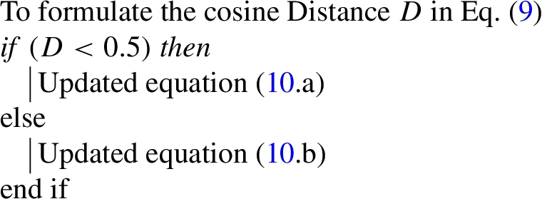
Improved cosine distance In improved cosine distance, first we calculated the distance value D, in Eq. (9). This distance value D is compared with the default threshold value 0.5. The improved cosine distance is formulated in Eq. (10). $\begin{array}{l} (9) & D = 1 - \frac{\sum p_{i} * q_{i}}{\sqrt{\sum {(p_{i})}^{2}} * \sqrt{\sum {(q_{i})}^{2}}} \\ (10) & ICD = \{\begin{matrix} (1 - D) * (D * D) + (D * \sqrt{D}), & if D < 0.5 \\ \sqrt{D}, & otherwise \end{matrix}\} \end{array}$ The output of the image segmentation process is $L_{S}$ .

Algorithm 1

Pseudo code of improved cosine distance

3.3. Feature extraction

The segmented output $L_{S}$ is the input of feature extraction phase. Here we extract the features like Improved Gabor Transitional Pattern, GLSM, statistical features and CNN based features.

3.3.1. Improved Gabor transitional pattern

The segmented image was subjected to a Gabor filter, and features were extracted using LTP code that was generated from the filtered image. Eight distinct orientations of the image were given the Gabor filter, which was then applied, and the resulting filtered images were then superimposed to create one final image [3].

LTP creates a texture code by comparing the intensity transition between adjacent pixels moving in different directions at different levels. Given image $L_{s} (x, y)$ , the LTP can calculated in Eq. (11) where, the $(x_{e}, y_{e})$ center pixel’s intensity value is denoted as j, $j 1$ and $j 2$ corresponds to the intensity values of P. The symbol ⊗ represents exclusive OR operation. $\begin{matrix} (11) & LTP (x_{e}, y_{e}) = \sum_{f = 0}^{f - 1} s (j_{f 1} - j_{e}) \otimes s (j_{f 2} - j_{e}) * 2^{f} \end{matrix}$ The improved LTP is represented in Eq. (12) where, $mMAD$ is modified Mad, which is represented in Eq. (13) here $\bar{g}$ is the weighted geometric mean of pixels, which is calculated in Eq. (14) $\begin{array}{l} (12) & {IG}_{F} = \sum_{f = 0}^{f - 1} s (j_{f 1} - mMAD) \otimes s (j_{f 2} - mMAD) * 2^{f} \\ (13) & mMAD = Median (| j_{i} - \bar{j} |) \\ (14) & \overline{j} = exp (\frac{\sum_{i = 1}^{n} w_{i} l n x_{i}}{\sum_{i = 1}^{n} w_{i}}) \end{array}$ ${IG}_{F}$ indicates the extracted feature.

3.3.2. Gray level co-occurrence matrices (GLCM)

A well-known statistical technique for extracting second-order texture information from a picture is the GLCM. It is shown as a matrix, with the number of columns and rows corresponding to the number of distinct grey levels or pixel values in a picture of a surface [15]. It describes how often a certain grey level will appear in a specific spatial linear relationship with a different grey level inside the study area. In this proposed work, we extract some features like energy, contrast, correlation, homogeneity and dissimilarity. These features are explained as follows.

Energy The score increases as the image becomes more homogeneous. The image is meant to remain constant when the energy is equal to one. It is calculated in Eq. (12) where, $N_{s}$ indicates the number of discrete intensity level of the image, the co-occurrence matrix is $P (x, y)$ , row is indicated as x and column is indicated as y $\begin{matrix} (15) & E^{i} = \sqrt{\sum_{x = 1}^{N_{s}} \sum_{y = 1}^{N_{s}} P {(x, y)}^{2}} \end{matrix}$

Contrast The term “contrast” is used to describe how an image’s input image’s intensity of a pixel and its neighbor is calculated. It is expressed in Eq. (16) $\begin{matrix} (16) & {CO}^{i} = \sum_{x = 1}^{N_{s}} \sum_{y = 1}^{N_{s}} | x - y |^{2} P (x, y) \end{matrix}$

Correlation The correlation texture determines how linearly or spatially related adjacent pixels’ grey levels are to one another. The correlation is evaluated in Eq. (17), Where $μ_{x} (u)$ and $μ_{y} (v)$ indicates the mean value of $(x)$ and $(v)$ , $σ_{u} (x)$ and $σ_{v} (y)$ indicates the SD of $(x)$ and $(y)$ $\begin{matrix} (17) & {CR}^{i} = \frac{\sum_{x = 1}^{N_{s}} \sum_{y = 1}^{N_{s}} x y P (x, y) - μ_{u} (x) μ_{v} (y)}{σ_{u} (y) σ_{v} (y)} \end{matrix}$

Homogeneity An image’s local homogeneity is measured by homogeneity. It is high when both the local grey level and its inverse, GLCM, are uniform. Whether the supplied image is textured or not will determine whether it has a single value or a range of values. It is evaluated in Eq. (18). $\begin{matrix} (18) & H^{i} = \sum_{x = 1}^{N_{s}} \sum_{y = 1}^{N_{s}} \frac{P (x, y)}{1 + | x - y |} \end{matrix}$

Dissimilarity It is a textural aspect of a picture that is calculated by taking the image’s arrangement into account as expressed in terms of an angle. It is calculated in Eq. (19) $\begin{matrix} (19) & D^{i} = \sum_{x = 1}^{N_{s}} \sum_{y = 1}^{N_{s}} (x - y) P (x, y) \end{matrix}$ In GLCM, the extracted features are represented in Eq. (20) $\begin{matrix} (20) & GLCM = E^{i} + {CO}^{i} + {CR}^{i} + H^{i} + D^{i} \end{matrix}$

3.3.3. Statistical features

In feature extraction phase, we are considering some statistical features namely, mean, median, standard deviation, skewness and kurtosis.

Mean ( $S_{1}$ ) For a set of limited data, the statistical mean – also known as the arithmetic average – measures central tendency. In order to calculate it, divide the dataset’s sum by the total number of values. The mean value is calculated in Eq. (21) Where, m indicates the count of provided dataset. $y_{i}$ indicates the given data set. $\begin{matrix} (21) & S_{1} = \frac{1}{m} \sum_{i = 1}^{m} y_{i} \end{matrix}$

Median ( $S_{2}$ ) A probability distribution or a population of data are divided into upper and lower halves by a number known as the median in statistics and probability theory. The value might bet the middle of the given data set. The Median value is calculated in Eq. (22) where m indicates the count of the given data set. $\begin{matrix} (22) & S_{2} = \frac{y_{(m + 1)}}{2} \end{matrix}$

Standard deviation ( $S_{3}$ ) An indicator of how much variety or dispersion there is in a set of numbers is the standard deviation (SD). The SD of a probability distribution, random values, collection of data, or statistical population is equal to its variance, squared. The SD will be measured by the Eq. (23) $\begin{matrix} (23) & S_{4} = \sqrt{\frac{\sum (y - S_{1})}{m}} \end{matrix}$

Skewness ( $S_{4}$ ) In probability theory and statistics, the term “skewness” is used to characterize an asymmetry between a probability density and the mean of a real-valued random variable. The skewness value may be indefinable, positive, zero, or any combination of the four. The Skewness value is determined by the Eq. (24) Where, $S_{e}$ is represented in Eq. (25) Here, the positive sample is indicated as PS and the negative sample is indicated as FS. $\begin{array}{l} (24) & {Sk}_{3} = \frac{\sum_{m = 1}^{M} {(s_{e} - s_{1})}^{3}}{(M - 1) s_{3}^{3}} \\ (25) & S_{e} = \frac{PS}{PS + FS} \end{array}$

Kurtosis ( $S_{5}$ ) A real-valued random variable’s kurtosis serves as a gauge for how “tailed” its probability distribution is. Equation (26) evaluate the value of Kurtosis. $\begin{matrix} (26) & Ku = \frac{\sum_{m = 1}^{M} {(s_{e} - s_{1})}^{4}}{(M - 1) s_{3}^{4}} \end{matrix}$ The extracted statistical feature is $S_{F} = S_{1} + S_{2} + S_{3} + S_{4} + S_{5}$

3.3.4. CNN based features

CNNs, a subset of deep feed-forward ANN, are frequently employed in computer vision tasks including image categorization [19]. CNN has input, convolutional, pooling, fully connected, and output layers, which sets it apart from a “simple” multilayer perception (MLP) network. Figure 2 shows the architecture of CNN model for Features Extraction.

Fig. 2.

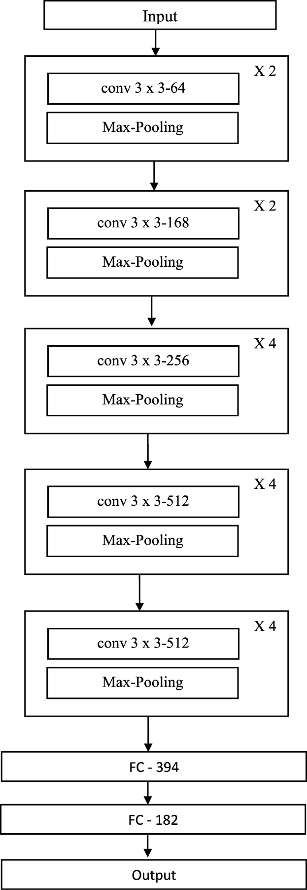
Architecture of CNN model for features extraction.

The CNN is fed an input image via the input layer. To prepare the input image as an acceptable data type for the CNN, it consists of a variety of low-level image processing operations. In order to ensure that a CNN can be computed efficiently, the size of the input image should ideally be a power of 2. But the most recent CNNs can also employ input images with irregular row-column dimensions.The output layer presents the extracted features from the input image.

3.4. Classification

In this classification stage, we combine two classifiers that is Bi-GRU and Deepmaxout network. Here the weight of both two classifiers can be tuned by using self improved COOT algorithm.

3.4.1. Bi-GRU

The processing of sequential data is a capability of RNNs. In addition, when dealing with new data, RNNs are able to draw some knowledge from earlier image [20]. Improved RNN models like the LSTM and GRU have strong modeling skills for long-term dependencies, while GRU is a less sophisticated variation than LSTM. A GRU is the combination of reset gate $(r_{t})$ and update gate $(z_{t})$ . By the use of current input $(x_{t})$ and previous state $(h_{t - 1})$ , the output $(h_{t})$ is calculated. The GRU unit is calculated in the following Eq. (27) where $W_{r}$ , $U_{r}$ , $W_{z}$ , $U_{z}$ , $W_{h}$ and $U_{h}$ are indicates the weight matrices, which is tuned by self improved COOT optimization algorithm. The bias vector is indicated as $b_{r}$ , $b_{z}$ , and $b_{h}$ , $x_{t}$ denote the input, $h_{t - 1}$ denoted the previous state, sigmoid function is denoted as σ, tangent activation function is denoted as tanh, ⊙ denotes the Hadamard product. $\begin{matrix} (27) & \begin{array}{l} r_{t} = σ (W_{r} x_{t} + U_{r} h_{t - 1} + b_{r}) \\ z_{t} = σ (W_{r} x_{t} + U_{r} h_{t - 1} + b_{z}) \\ {\tilde{h}}_{t} = tanh [W_{h} x_{t} + U_{h} (r_{t} ⊙ h_{t - 1}) + b_{h}] \\ h_{t} = (1 - z_{t}) ⊙ h_{t - 1} + z_{t} ⊙ {\tilde{h}}_{t} \end{array}\} \end{matrix}$

Models having a bi-directional structure are able to use knowledge from the prior and the future while interpreting the data at hand. The first GRU starts moving forward at the beginning of the data series, while the second GRU starts moving backward at the end of the data series. Due to this, information from the past and the future might have an impact on the circumstances of the present. The bi-GRU is defined in the following Eq. (28), where ${\vec{h}}_{t}$ and $\overset{\leftarrow}{h_{t}}$ are the both forward and backward states, ⊕ denotes the operation of concatenating two vectors. $\begin{matrix} (28) & \begin{array}{l} {\vec{h}}_{t} = {GRU}_{fwd} (x_{t}, \vec{h_{t - 1}}) \\ {\overset{\leftarrow}{h}}_{t} = {GRU}_{bwd} (x_{t}, \overset{\leftarrow}{h_{t + 1}}) \\ h_{t} = {\vec{h}}_{t} \oplus {\overset{\leftarrow}{h}}_{t} \end{array}\} \end{matrix}$

3.4.2. Deep maxout

In deep maxout neural network, every neuron has a group, which including of K candidate pieces [5]. Depending on the highest value, the neuron activation value is calculated, which is obtained from all k pieces. The link between the $i^{th}$ node of the $l^{th}$ hidden layer as $h_{l}^{i}$ and its associated components, denoted as $z_{l}^{i j}$ , is consistent. It is represented in Eq. (29). Where $Z_{l}^{i j}$ is calculated by forward propagation from the Eq. (30) where $z_{l} \in R^{z}$ , $h_{l - 1} \in R^{H}$ , $W_{l - 1} \in R^{H \times Z}$ here the weights are tuned by self improved COOT optimization algorithm, $b_{l} \in R^{Z}$ . $\begin{array}{l} (29) & h_{l}^{i} = max_{j \in 1 \dots k} z_{l}^{i j} \\ (30) & z_{l} = W_{l - 1}^{T} h_{l - 1} + b_{l} \end{array}$

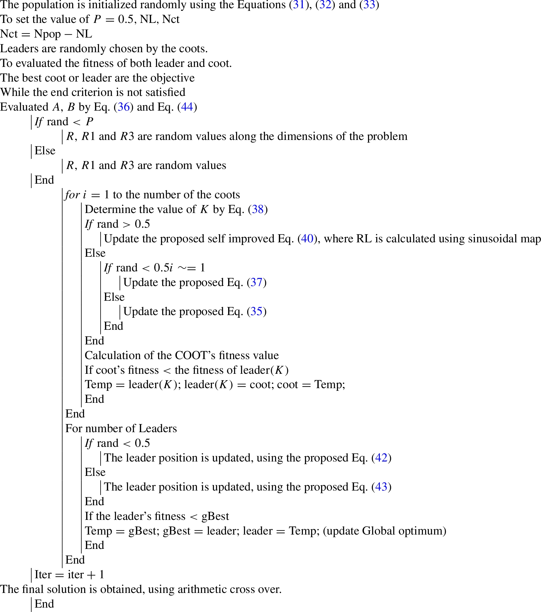
Only the weights related to the component with the maximum activation within every group ${z_{l}^{i j} | j \in 1 \dots k}$ for $l \in [1, L]$ and $i \in [1, N^{l}]$ are updated throughout the back-propagation procedure during training, which always has a gradient of 1. In convolutional networks, this is comparable to max-pooling. In contrast, max-pooling in convolutional networks occurs across spatial locations, but max-pooling in maxout networks occurs across k pieces, which are comparable to distinct features inside a single spatial region.

4. Crossover mutated COOT optimization (CMCO)

In classification phase, the self improved COOT optimization algorithm is used to tune the weight of both two classifiers that is Bi-GRU and Deep Maxout.

The Coots are little waterfowl that belong to the Rallidae family of rails [23]. The underside of the tail is often white, but not always. Coots reveal a range of actions and behaviors when they are on the water. Using the movement of this coot on the water’s surface, a novel optimization technique is demonstrated in this research. Surf scoters sense a region of repulsion when coots move at angle to their movement direction. This suggests that coots approach quite close to this zone. When coots swarm on water, they move in three different ways. Each coot follows its front coot as a chain of coots glides across the water. Humans see the coots in the front of the flock as the group’s leaders since they are in charge of guiding the entire flock in the right direction. The four unique motions that birds make on the water’s surface are now taken into consideration. The movements are

Random swaying to one side or the other

Chain Movement

depending on the group leaders, changing the position

the group’s leaders directing them to the ideal location

Mathematical model The method starts from a random population. This random population is evaluated iteratively by the target function to provide the desired result. A collection of principles that form the basis of an optimization process also improves it. There is no assurance that a result will be discovered in a single run because population-based optimization techniques hunt for the right number of optimization issues. On the other hand, with enough random values and optimization steps, the chance of achieving the overall optimum increases. In Eq. (31), the population is generated by randomly in the space. Where, the coot’s position is denoted as $LP (i)$ . d indicates the problem dimensions or variables, lower bound value is indicated as $lb$ , the upper bound value is indicated as $ub$ . Both $lb$ and $ub$ are evaluated in the following Eq. (32) and (33) $\begin{array}{l} (31) & LP (i) = rand (1, d) * (ub - lb) + lb \\ (32) & lb = [{lb}_{1}, {lb}_{2}, \dots, {lb}_{d}] \\ (33) & ub = [{ub}_{1}, {ub}_{2}, \dots, {ub}_{d}] \end{array}$

Using the objective function, it is necessary to assess each solution’s efficiency after the initial population is generated and each agent is placed. Group leaders are chosen from the $NL$ number of coots. Leader selection is random.

4.1. Proposed random swaying to one side or the other

We use Eq. (34) to select a random location within the search area and move the coot there to complete this movement. $\begin{matrix} (34) & Q = rand (1, d) * (ub - lb) + lb \end{matrix}$

This movement of the coot covers a wide portion of the search space. The algorithm can use this motion to escape the localized optimal if it ever catches itself there. Using Eq. (35), coot’s new location is calculated. Where $R 2$ indicates random value between 0 to 1 is, A is calculated using the self improved Eq. (36) where, the current iteration indicated as L and the maximum iteration is denoted as $Iter$ . $\begin{array}{l} (35) & LP (i) = LP (i) + A \times R 2 \times (Q - LP (i)) \\ (36) & A = \frac{1.5 * Iter - L + 1}{Iter} \end{array}$

4.2. Chain movement

This movement can be created using the average position of two coots. Another method for establishing a chain movement is to calculate the distance of two coots and then it moves to the other distance that is half of that distance. We used the first method, and a equation (37) was calculate the coot’s new position. Where $LP (i - 1)$ denotes the second coot. $\begin{matrix} (37) & LP (i) = 0.5 \times (LP (i - 1) + LP (i)) \end{matrix}$

4.3. Proposed method depending on the group leaders, changing the position

After shifting their postures to align with the group leaders, who are typically a few coots ahead of the group, the majority of the coots must advance towards the leaders. One conceivable question is if each coot’s position will change based on which leader is in control. The coots might adjust their position in light of the overall average of the leaders, which can be taken into consideration. Convergence happens too soon when using the average position. Using Eq. (38) implement this movement. Where coot’s index number is denoted as i, number of leaders denoted as $NL$ and Leader’s index number is denoted as K. Using Eq. (39) coot’s next position will be found based on the chosen leader, which is updated by self improved Eq. (40) Where R1 is a random number, which is calculated using sinusoidal Map in Eq. (41). All parallels and the centre meridian are shown at real scale in the sinusoidal projection, which is a pseudocylindrical equal-area projection. A significant shape distortion is produced close to the map’s outline by the boundary meridians’ severe outward bulging. The continuity of the projection over the oceans is broken in other formats, which also centre the continents around their own central meridian lines, or vice versa, to lessen distortion along outer meridian lines. $\begin{array}{l} (38) & K = 1 + (i MOD NL) \\ (39) & Cootposold = Leaderpos (K) + 2 \times R 1 \times cos (2 R π) \times (Leaderpos (K) - Cootpos (i)) \\ (40) & LP (i) = LP (i) + R_{L} * (Leaderpos (k) - LP (i) + rand (- 1, 1) * Cootposold - LP (i)) \\ (41) & RL = 2.3 * r^{2} . sin (π r) \end{array}$

4.4. The group’s leaders directing them to the ideal location

To direct the group in the right direction, leaders must adjust their own position in respect to the objective. Using For Eq. (42) and Eq. (43), it is suggested that leadership roles be updated. This equation seeks out better locations in the immediate area of the present optimal point. By using this approach, you can move both in the direction of and far from the optimal location. Where, the best position is denoted as $gbest$ . The random value between 0 to 1 is assigned to $R 3$ and $R 4$ . R indicates the random number between −1, 1 and B is calculated using the Eq. (44) where, the current iteration is denoted as L, and maximum number of iteration is denoted as $Iter$ . $\begin{array}{l} (42) & Leaderpos (i) = {B \times R 3 \times cos (2 R π) \times (gBest - Leaderpos (i)) + gBest, R 4 < 0.5} \\ (43) & Leaderpos (i) = {B \times R 3 \times cos (2 R π) \times (gBest - Leaderpos (i)) - gBest, R 4 ⩾ 0.5} \\ (44) & B = 2 - L \times (\frac{1}{Iter}) \end{array}$

To retain the randomness of the selection procedure, we treat each of these movements as if it were a random occurrence. During the course of the algorithm, the coot may begin to migrate in a chain or in the direction of group leaders.

In the end, the solution is discovered by applying arithmetic cross over. To integrate the two parent chromosomes linearly, a crossover operator in arithmetic is used. The crossover operator in arithmetic is a linear combination of the two parent chromosomes. An arithmetic crossover involves the selection of two chromosomes at random for crossover, which are subsequently united in a linear manner to produce two offspring. It is represented in Eq. (45). Where $\bar{x}$ and $\bar{y}$ denotes mom and dad. α is generated by randomly between 0 and 1. $\begin{matrix} (45) & offspring = α . \bar{x} + (1 - α) . \bar{y} \end{matrix}$

Algorithm 2

Pseudo code of CMCO

Figure 3 shows the flowchart of the proposed model.

Fig. 3.

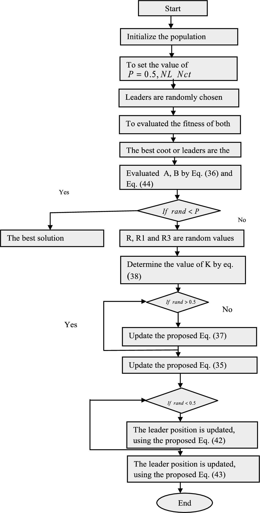
Flowchart of the proposed model.

5. Result and discussion

Further, the investigation was carried out regarding positive measure, negative measure and other measures as well as the results related to the corresponding simulation were observed.

5.1. Simulation procedure

The proposed based Liver cancer classification model was executed in PYTHON and the dataset was gathered in [1]. The CMCO was estimated over the Aquila Optimizer (AO), Chimp Optimization Algorithm (COA), Tunicate Swarm Algorithm (TSA), Archimedes Optimization Algorithm (AOA) and COOT. The Liver Cancer classification images are displayed in Fig. 4.

Fig. 4.

Images for liver cancer classification a) input image b) preprocessed image c) conventional segmented image d) K-means segmented Image e) watershed segmented image f) CMCO segmented image.

5.2. Dataset description

“The DeepLesion dataset contains 32,120 axial computed tomography (CT) slices from 10,594 CT scans (studies) of 4,427 unique patients. There are 1–3 lesions in each image with accompanying bounding boxes and size measurements, adding up to 32,735 lesions altogether. The lesion annotations were mined from NIH’s picture archiving and communication system (PACS).”

5.3. Analysis on positive measure of CMCO over the standard methods by adjusting the learning percentage

The study on CMCO is computed over the extant schemes like AO, COA, TSA, AOA and COOT for diverse learning percentages are represented in Fig. 5. For enhanced system performance, the positive metric needs to be high. While assessing the Fig. 5, the CMCO and other established schemes have obtained maximal positive measure ratings i.e. greater than 80%. However, the CMCO accomplished the greater positive metric values than the current strategies. The CMCO obtained the greatest specificity at the 80th learning percentage is about 92.97%, this is superior to AO = 89.09%, COA = 86.11%, TSA = 84.43%, AOA = 88.59% and COOT = 88.73%, respectively. Regarding the Fig. 5(b), with the learning percentage of 90%, the models like AO, COA, TSA, AOA and COOT attained the minimal precision of 92.81%, 90.05%, 88.76%, 92.74% and 92.67%, whilst the CMCO reached the highest level of precision is 96.20%.

Furthermore, evaluating the sensitivity and accuracy measure of the CMCO and the traditional methodologies as well as the corresponding results are shown in Fig. 5(c) and 5(d). In the 70% of learning percentage, the CMCO generated the sensitivity of 95.17%, even though the standard schemes scored minimum sensitivity, including, AO is 92.05%, COA is 89.11%, TSA is 87.50%, AOA is 92.24% and COOT is 91.75%, respectively. Particularly, the CMCO obtained the sensitivity of 90.83% in the 60th learning percentage, although it attained the maximal sensitivity at the 90th learning percentage is 96.50%. For the learning percentage 90, the CMCO gained the accuracy of 95.58%, which is preferable than AO = 92.16%, COA = 89.38%, TSA = 88.05%, AOA = 92.05% and COOT = 91.95%, respectively. As we have accomplished improvements in segmentation with enhanced feature extraction, the resultants of the CMCO is more appealing than those of the others strategies.

Fig. 5.

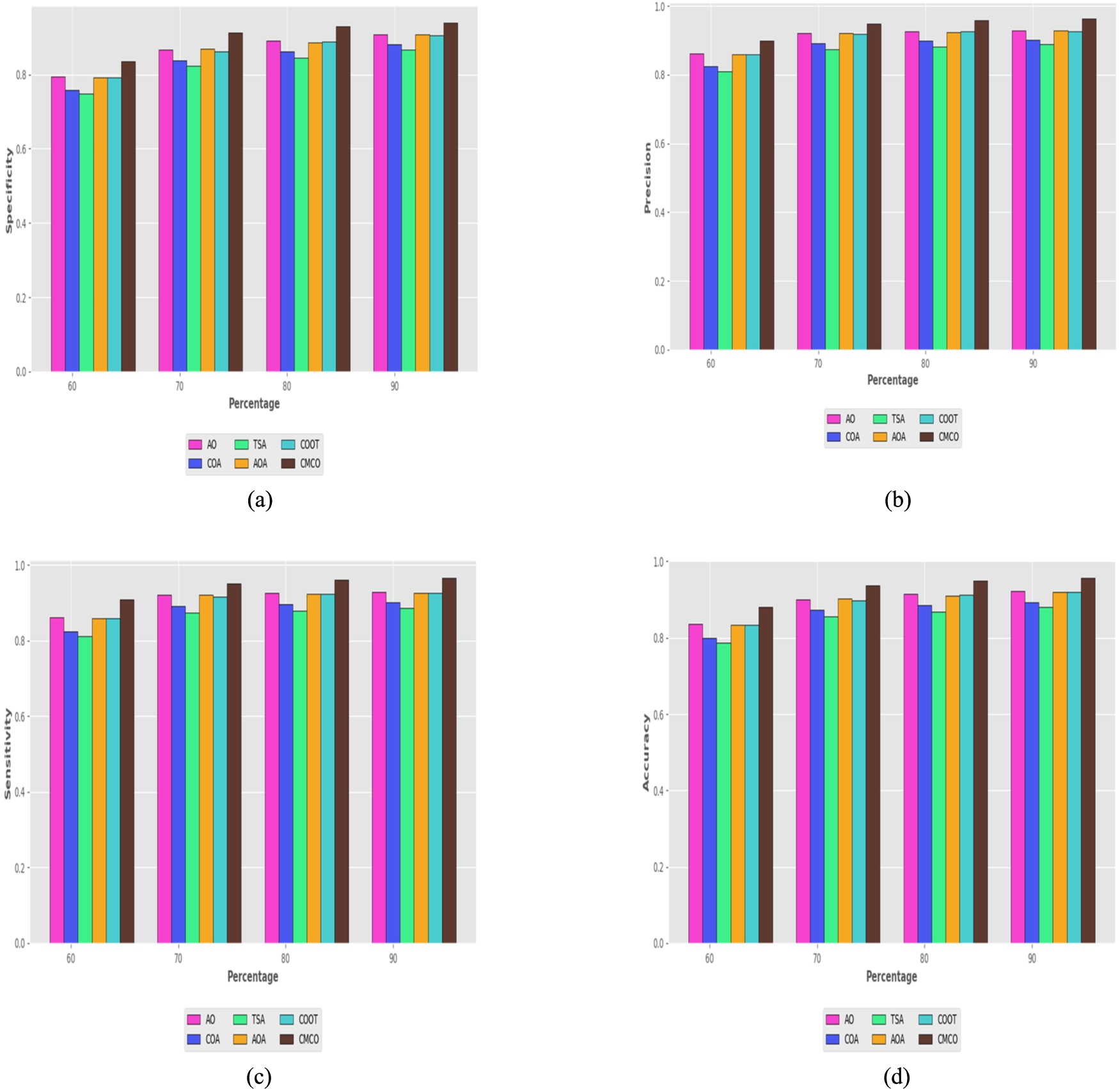
Assessment on positive measure of the CMCO versus traditional methods a) specificity b) precision c) sensitivity d) accuracy by varying the learning percentage.

5.4. Analysis on negative measure of CMCO over the standard methods by adjusting the learning percentage

The negative measure (FNR and FPR) analysis of the CMCO is conflicts with the AO, COA, TSA, AOA and COOT is exposed in Fig. 6. Here, the negative measures should be lower for better liver cancer classification system. Likewise, the CMCO attained the minimal FNR and FPR in almost all the learning percentages; thereby it is preferable approach for liver cancer classification. As stated by the Fig. 6(a), the FNR of the CMCO for the 80th learning percentage is 3.94191, whilst the traditional approaches attained the lowest FNR error rate, such as, AO = 7.249945, COA = 10.2411, TSA = 11.9651, AOA = 7.587618 and COOT = 7.495715, respectively. The minimal FPR is acquired by the CMCO ranging from 16.5334 to 6.18034. Particularly, at the 80% of learning percentage, the CMCO yielded the FPR of 7.029402, even though the AO = 10.9082, COA = 3.88575, TSA = 15.56878, AOA = 11.40086 and COOT = 11.26711, respectively. Nearly in all error measurements, the CMCO model shows its superior performance. This exhibits that the CMCO might be more specific with its contributions on resolving the specified classification problem more effectively.

Fig. 6.

Assessment on positive measure of the CMCO versus traditional methods a) FNR b) FPR by varying the learning percentage.

5.5. Analysis on other measure for CMCO over the standard methods by adjusting the learning percentage

The other measure evaluation of the CMCO is compared to the AO, COA, TSA, AOA and COOT by adjusting the learning percentage and the findings are presented in Fig. 7. Here, the CMCO has generated better values than the other five previous algorithms. While fixing the learning percentage to 60%, the CMCO acquired the F-measure of 90.39%, even thought the AO is 86.13%, COA is 82.43%, TSA is 81.08%, AOA is 85.89% and COOT is 85.87%, respectively. Similarly, the NPV of the CMCO is 90.88% (Learning percentage = 90%), surpassing the AO = 90.88%, COA = 88.07%, TSA = 86.67%, AOA = 90.70% and COOT = 90.53%, respectively. Simultaneously, the CMCO attained the highest MCC of 91.65% at the 90% of learning percentage, whilst it attained 76.41%, 87.99% and 90.43% of precision at the 60, 70 and 80% of learning percentage. Nevertheless, the CMCO obtained the greatest MCC in all the learning percentages. This has clearly proven that the CMCO is efficacious in classifying liver cancer with improved segmentation as it has gotten the greatest other metrics compared to the other established approaches.

Fig. 7.

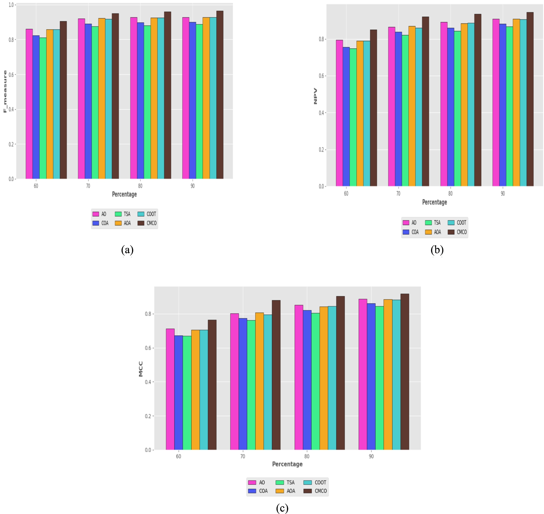
Assessment on positive measure of the CMCO versus traditional methods a) F-measure b) NPV c) MCC by varying the learning percentage.

5.6. Ablation study on CMCO, model with conventional segmentation, model with conventional LGTrP and model without optimization for varied measures

The ablation study on CMCO, model with conventional segmentation, model with conventional LGTrP and model without optimization for distinctive measures are overviewed in Table 2. The accuracy of the model with conventional segmentation is 87.11%, model with conventional LGTrP is 86.25%, model without optimization is 81.70% and CMCO is 93.81%, respectively. Furthermore, the model with conventional segmentation, model with conventional LGTrP, model without optimization and CMCO recorded the FPR of 0.176463, 0.186841, 0.239737 and 0.087277, respectively. To improve the efficiency of the liver disease classification deep fuzzy clustering is used. For extracting the features, improved Gabor Transitional Pattern is used and the optimization is carried out to tune the weight of the classifiers. Further, it can be ascertained that the CMCO with the entire presented enhancement can contribute to incredible outcomes.

Table 2
Ablation study on CMCO, model with conventional segmentation, model with conventional LGTrP and model without optimization for varied positive, negative and other measure

Model with conventional segmentation Model with conventional LGTrP Model without optimization CMCO

Accuracy 0.871138 0.862508 0.817038 0.938197

MCC 0.719018 0.700688 0.605715 0.879992

Precision 0.902732 0.896681 0.862433 0.947414

F-measure 0.900066 0.89319 0.855884 0.94956

Specificity 0.823537 0.813159 0.760263 0.912723

NPV 0.814241 0.801674 0.739224 0.920529

FPR 0.176463 0.186841 0.239737 0.087277

Sensitivity 0.897575 0.88992 0.849567 0.951719

FNR 0.102425 0.11008 0.150433 0.048281

	Model with conventional segmentation	Model with conventional LGTrP	Model without optimization	CMCO
Accuracy	0.871138	0.862508	0.817038	0.938197
MCC	0.719018	0.700688	0.605715	0.879992
Precision	0.902732	0.896681	0.862433	0.947414
F-measure	0.900066	0.89319	0.855884	0.94956
Specificity	0.823537	0.813159	0.760263	0.912723
NPV	0.814241	0.801674	0.739224	0.920529
FPR	0.176463	0.186841	0.239737	0.087277
Sensitivity	0.897575	0.88992	0.849567	0.951719
FNR	0.102425	0.11008	0.150433	0.048281

5.7. Classifier comparison on CMCO and the standard classifiers for various measures

The performance of CMCO for Liver cancer classification is compared over KNN, CNN, RNN, Bi-GRU, Deep Maxout, HFCNN [12] and NBC-DNN [10] for various types of metrics is depicted in Table 3. In order for the system to perform effectively, both the positive and other metrics should be maximized, as well as the negative measure must be minimized. Especially, the precision of the CMCO is 94.74%, whilst the KNN = 86.09%, CNN = 85.47%, RNN = 84.28%, Bi-GRU = 85.57%, Deep Maxout = 86.47%, HFCNN = 79.52% and NBC-DNN = 75.63%, respectively. Moreover, the FNR of the CMCO is 0.048281, mean while the standard approaches like KNN, CNN, RNN, Bi-GRU, Deep Maxout, HFCNN and NBC-DNN obtained the FNR of 0.149833, 0.1546402, 0.159708, 0.155306, 0.085832, 0.127165 and 0.149468, respectively. Subsequently, the Accuracy, NPV and FPR acquired by the CMCO is 93.81%, 92.05% and 0.087277. This confirms that the CMCO provided improved accuracy with reduced error rate.

Table 3
Classifier comparison on CMCO versus established classifiers for positive, negative and other measures

KNN CNN RNN Bi-GRU Deep maxout HFCNN [12] NBC-DNN [10] CMCO

Accuracy 0.816197 0.808474 0.799374 0.80976 0.896616 0.844942 0.816626 0.938197

MCC 0.603126 0.587076 0.568088 0.589746 0.775086 0.66482 0.604019 0.879992

Precision 0.860917 0.854739 0.842881 0.855769 0.924789 0.883727 0.861259 0.947414

F-measure 0.855508 0.849132 0.841585 0.850195 0.919447 0.878247 0.855862 0.94956

Specificity 0.755798 0.746326 0.728431 0.747899 0.864752 0.795232 0.756326 0.912723

NPV 0.739383 0.729503 0.724572 0.731143 0.846483 0.777863 0.739935 0.920529

FPR 0.244202 0.253674 0.271569 0.252101 0.135248 0.204768 0.243674 0.087277

Sensitivity 0.850167 0.843598 0.840292 0.844694 0.914168 0.872835 0.850532 0.951719

FNR 0.149833 0.156402 0.159708 0.155306 0.085832 0.127165 0.149468 0.048281

	KNN	CNN	RNN	Bi-GRU	Deep maxout	HFCNN [12]	NBC-DNN [10]	CMCO
Accuracy	0.816197	0.808474	0.799374	0.80976	0.896616	0.844942	0.816626	0.938197
MCC	0.603126	0.587076	0.568088	0.589746	0.775086	0.66482	0.604019	0.879992
Precision	0.860917	0.854739	0.842881	0.855769	0.924789	0.883727	0.861259	0.947414
F-measure	0.855508	0.849132	0.841585	0.850195	0.919447	0.878247	0.855862	0.94956
Specificity	0.755798	0.746326	0.728431	0.747899	0.864752	0.795232	0.756326	0.912723
NPV	0.739383	0.729503	0.724572	0.731143	0.846483	0.777863	0.739935	0.920529
FPR	0.244202	0.253674	0.271569	0.252101	0.135248	0.204768	0.243674	0.087277
Sensitivity	0.850167	0.843598	0.840292	0.844694	0.914168	0.872835	0.850532	0.951719
FNR	0.149833	0.156402	0.159708	0.155306	0.085832	0.127165	0.149468	0.048281

5.8. Statistical assessment on CMCO and the conventional methods in terms of error for various case scenarios

The statistical evaluation of the CMCO is associated to the AO, COA, TSA, AOA and COOT under the mean, standard deviation, maximum, median and minimum case scenario is represented in Table 4. Regarding the statistical evaluation, the CMCO obtained the lowest error value for liver cancer classification system than the conventional schemes. In accordance with the minimum case scenario, the CMCO generated the error rate of 1.075606, even though the traditional methodologies acquired maximal error rate, namely, AO is 1.091018, COA is 1.099898, TSA is 1.086785, AOA is 1.082553 and COOT is 1.080126, respectively. Additionally, the CMCO recorded the minimal error rate under the mean case scenario is 1.085719, though the AO is 1.103969, COA is 1.143674, TSA is 1.097733, AOA is 1.098426 and COOT is 1.090266, respectively. Finally, it establishes that the CMCO has the adequacy to diminish the error even in the complicated scenarios.

Table 4
Statistical assessment on CMCO over the conventional schemes for mean, standard deviation, maximum, median and minimum case scenario

Mean Maximum Standard deviation Median Minimum

AO 1.103969 1.176596 0.025368 1.091018 1.091018

COA 1.143674 1.200135 0.04736 1.106375 1.099898

TSA 1.097733 1.125523 0.016045 1.086785 1.086785

AOA 1.098426 1.146351 0.022588 1.082553 1.082553

COOT 1.090266 1.135598 0.02146 1.080126 1.080126

CMCO 1.085719 1.140562 0.019114 1.077793 1.075606

	Mean	Maximum	Standard deviation	Median	Minimum
AO	1.103969	1.176596	0.025368	1.091018	1.091018
COA	1.143674	1.200135	0.04736	1.106375	1.099898
TSA	1.097733	1.125523	0.016045	1.086785	1.086785
AOA	1.098426	1.146351	0.022588	1.082553	1.082553
COOT	1.090266	1.135598	0.02146	1.080126	1.080126
CMCO	1.085719	1.140562	0.019114	1.077793	1.075606

5.9. Convergence study on CMCO and current schemes by varying the iteration

The convergence evaluation of the CMCO is assessed over the AO, COA, TSA, AOA and COOT is portrayed in Fig. 8. Here, the iteration ranges from 0 to 50. For an improved liver cancer categorization system, the error rate should be as low as possible. The CMCO and other classifiers acquired the highest error rate from the iteration 0 to 30, however as the number of iterations progressed, the error rate for all the classifiers dropped. Whatever, the error rate of the CMCO is 1.076, mean while the conventional approaches has obtained the highest error value, notably, AO = 1.098, COA = 1.087, TSA = 1.084, AOA = 1.082 and COOT = 1.080, respectively. The CMCO has asserted its advancement with better convergence rate and quickness to reach the error specified in the classification process.

Fig. 8.

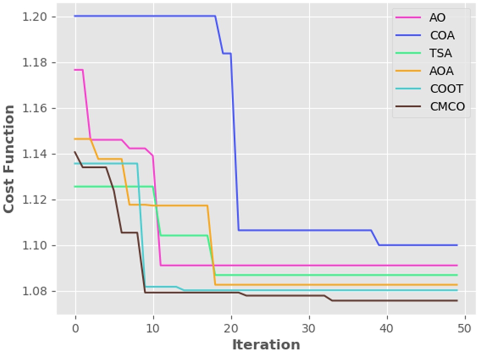
Convergence evaluation on CMCO versus traditional methodologies by modifying the iterations.

5.10. ROC and AUC analysis

The receiver operating characteristic curve (ROC curve) is a graph that displays how well a classification model performs across all categorization levels. The abbreviation “Area under the ROC Curve” is AUC. In other words, AUC calculates the area in two dimensions underneath the complete ROC curve. Instead of assessing predictions’ absolute values, it assesses how well they are rated. Figure 9 deploys the ROC and AUC analysis.

Fig. 9.

ROC and AUC analysis.

Table 5

Nomenclature

CAD	Computer Assisted Diagnosis
Chi2	Chi-Squared
CLAHE	Contrast Limited Adaptive Histogram Equalization
CNN	Convolutional neural network
DL	Deep Learning
DNN	Deep Neural Network
DSFNN	Sunflower Optimization-based deep neural network
DTN	DNA tetrahedral nanostructure
FLC	Fibrolamellar HCC
FRET	Fluorescence Resonance Energy Transfer
GR	Gain Ratio
H&E	Hematoxylin and Eosin
HCC	Hepatocellular carcinoma
HCCCCA	Hepatocellular cholangiocarcinoma
HFCNN	Hybridized Fully Convolutional networks
HFCNN	Hybridized Fully Convolutional Neural Network
ICCA	Intrahepatic cholangiocarcinoma
IG	Information Gain
ML	Machine Learning
MSSO	Modified Social Ski-Driver optimization
RBC	Red Blood Cells
RF	RelieF
SERS	Surface-enhanced Raman spectroscopy
SU	Symmetrical Uncertainty
WHO	World Health Organization

6. Conclusion

Liver cancer predication is one of the most challenging tasks of the doctors. Liver cancer is mostly identified by the using of X-ray images or CT images. This paper proposed the technique for liver disease classification using CT images. It consists of four stages like preprocessing, segmentation, feature extraction and classification. In preprocessing stage, the input image was preprocessed and the quality of the image was improved. The preprocessed output was the input of the segmentation phase, here improved Deep fuzzy clustering method was used for image segmentation. The segmented output was subjected to the input of the feature extraction phase, where the extracted features are improved Gabor transitional pattern, GLCM, statistical features and CNN based features. This extracted feature was subjected to the input of the classification stage. In classification state we applied a crossover muted COOT optimization (CMCO) for tuning the weights. Finally the output image was presented the best accuracy of disease classification. Doctors can more easily create treatment plans by successfully classifying the various levels of differentiation, allowing patients to receive care on time. It can simultaneously reduce medical staff workload and the amount of time needed to look through liver cancer histopathological images.

References

https://nihcc.app.box.com/v/DeepLesion/folder/50715173939.

A.A.

Aatresh,

Alabhya,

Lal et al., LiverNet: Efficient and robust deep learning model for automatic diagnosis of sub-types of liver hepatocellular carcinoma cancer from H&E stained liver histopathology images, Int J CARS 16 (2021), 1549–1563. doi:10.1007/s11548-021-02410-4.

Ahsan,

Jabid and

U.P.

Chong, Facial expression recognition using local transitional pattern on Gabor filtered facial images, IETE Technical Review 30(1) (2013), 47–52. doi:10.4103/0256-4602.107339.

Alawneh,

Alquran,

Alsalatie,

W.A.

Mustafa,

Al-Issa,

Alqudah and

Badarneh, LiverNet: Diagnosis of liver tumors in human CT images, Applied Sciences 12(11) (2022), 5501. doi:10.3390/app12115501.

Cai,

Shi and

Liu, Deep maxout neural networks for speech recognition, in: IEEE Workshop on Automatic Speech Recognition and Understanding, 2013, pp. 291–296. doi:10.1109/ASRU.2013.6707745.

L.K.

Chan,

Y.M.

Tsui,

D.W.H.

Ho and

I.O.L.

Ng, Cellular heterogeneity and plasticity in liver cancer, in: Seminars in Cancer Biology, Vol. 82, Academic Press, 2021.

Chauhan ,

Chandra and

Kumar , Advanced electrochemical nanobiosensor for ultraefficient Annexin A2 biomarker detection: A rapid, label free and minimal invasive approach towards early diagnosis of liver cancer, Materials Letters 305 (2021).

Chen,

Ma,

Lv,

Dong,

Yan,

Zhu and

Chen, Classification of multi-diferentiated liver cancer pathological images based on deep learning attention mechanism, 2022.

Cheng ,

Chen ,

Lou ,

Fu and

Wang , A biosensing method for the direct serological detection of liver diseases by integrating a SERS-based sensor and a CNN classifier, Biosensors and Bioelectronics 186 (2021). doi:10.1016/j.bios.2021.113268.

10.

Cheng ,

Fu ,

Chen ,

Chen and

Wang , An antibody-free liver cancer screening approach based on nanoplasmonics biosensing chips via spectrum-based deep learning, NanoImpact 21 (2021). doi:10.1016/j.impact.2021.100296.

11.

Ding,

X.Y.

Zhang,

D.Y.

Wu and

M.L.

Liu, Application of an extreme learning machine network with particle swarm optimization in syndrome classification of primary liver cancer, Journal of Integrative Medicine 19 (2021). doi:10.1016/j.joim.2021.08.001.

12.

Dong,

Zhou,

Wang,

Peng,

Lou and

Fan, Liver cancer detection using hybridized fully convolutional neural network based on deep learning framework, IEEE Access 8 (2020), 129889–129898. doi:10.1109/ACCESS.2020.3006362.

13.

Fujita,

Yamaguchi,

Hasegawa,

Shimada,

Arihiro,

Hayashi,

Maejima,

Nakano,

Fujimoto,

Ono and

Aikata, Classification of primary liver cancer with immunosuppression mechanisms and correlation with genomic alterations, EBioMedicine 53 (2020).

14.

Gunasekhar and

Vijayalakshmi, Optimal biomarker selection using adaptive social ski-driver optimization for liver cancer detection, ScienceDirect 40 (2020).

15.

Gupta,

R.K.

Lama,

S.W.

Lee and

G.R.

Kwon, An MRI brain disease classification system using PDFB-CT and GLCM with kernel-SVM for medical decision support, Multimedia Tools and Applications 79(43) (2020), 32195–32224. doi:10.1007/s11042-020-09676-x.

16.

Hassan,

Ali,

Alquhayz,

J.Y.

Kim and

Sanaullah, Developing liver cancer drug response prediction system using late fusion of reduced deep features, Journal of King Saud University – Computer and Information Sciences 34 (2022).

17.

Hellingman,

M.E.

de Swart,

J.J.A.

Joosten,

M.R.

Meijerink,

J.J.J.

de Vries,

J.W.D.

de Waard,

A.A.

van Zweeden,

B.M.

Zonderhuis and

Kazemier, The value of a dedicated multidisciplinary expert panel to assess treatment strategy in patients suffering from colorectal cancer liver metastases, Surgical Oncology 35 (2020).

18.

Kaur,

A.P.S.

Chauhan and

A.K.

Aggarwal, An automated slice sorting technique for multi-slice computed tomography liver cancer images using convolutional network, Expert Systems With Applications 186 (2021).

19.

Khwildi,

A.O.

Zaid and

Dufaux, Query-by-example HDR image retrieval based on CNN, Multimedia Tools and Applications 80(10) (2021), 15413–15428. doi:10.1007/s11042-020-10416-4.

20.

Liu,

Wang,

Xu,

Li and

Xin, Bi-directional gated recurrent unit neural network based nonlinear equalizer for coherent optical communication system, Optics Express 29(4) (2021), 5923–5933. doi:10.1364/OE.416672.

21.

K.F.

Mahin ,

Robiuddin ,

Islam ,

Ashraf ,

Yeasmin ,

Shatabda , PanClassif: Improving pan cancer classification of single cell RNA-seq gene expression data using machine learning, Genomics 114 (2022).

22.

Mao,

Ma,

Duan et al., Preoperative classification of primary and metastatic liver cancer via machine learning-based ultrasound radiomics, EurRadiol 31 (2021), 4576–4586. doi:10.1007/s00330-020-07562-6.

23.

Naruei and

Keynia , A new optimization method based on COOT bird natural life model, Expert Systems With Applications 183 (2021).

24.

Othman,

Mahmoud,

Dhahri,

Abdulkader,

Mahmood and

Ibrahim, Automatic detection of liver cancer using hybrid pre-trained models, Sensors (2022).

25.

Rela,

S.N.

Rao and

R.R.

Patil, Performance analysis of liver tumor classification using machine learning algorithms, International Journal of Advanced Technology and Engineering Exploration 9(86) (2022), 143.

26.

Roy,

Das,

Lal et al., Novel edge detection method for nuclei segmentation of liver cancer histopathology images, J Ambient Intell Human Comput (2021). doi:10.1007/s12652-021-03308-4.

27.

Sun,

Xu,

Liu,

Xiong,

Zhao and

Ding, Deep learning-based classification of liver cancer histopathology images using only global labels, IEEE Journal of Biomedical and Health Informatics 24(6) (2020), 1643–1651. doi:10.1109/JBHI.2019.2949837.

28.

B.S.

Vidya and

Chandra, Triangular fuzzy membership-contrast limited adaptive histogram equalization (TFM-CLAHE) for enhancement of multimodal biometric images, Wireless Personal Communications 106(2) (2019), 651–680. doi:10.1007/s11277-019-06184-6.

29.

Wang,

Xu,

Wang and

Hua, Diketopyrrolopyrrole-based fluorescent probe for endogenous bisulfite detection and bisulfite triggered phototoxicity specific in liver cancer cells, Spectrochimica Acta Part A: Molecular and Biomolecular Spectroscopy 262 (2021).

30.

Zhang,

Wang,

Zhang,

Gao,

Wang and

Zhang, Improved fuzzy clustering for image segmentation based on a low-rank prior, Comp Visual Media 7 (2021), 513–528. doi:10.1007/s41095-021-0239-3.

31.

Zhao ,

Wang ,

Xiong ,

Liu and

Chen , Simultaneous fluorescent detection of multiplexed miRNA of liver cancer based on DNA tetrahedron nanotags, Talanta 210 (2020).