Projection decomposition algorithm for dual-energy computed tomography via deep neural network

Abstract

BACKGROUND:

Dual-energy computed tomography (DECT) has been widely used to improve identification of substances from different spectral information. Decomposition of the mixed test samples into two materials relies on a well-calibrated material decomposition function.

OBJECTIVE:

This work aims to establish and validate a data-driven algorithm for estimation of the decomposition function.

METHODS:

A deep neural network (DNN) consisting of two sub-nets is proposed to solve the projection decomposition problem. The compressing sub-net, substantially a stack auto-encoder (SAE), learns a compact representation of energy spectrum. The decomposing sub-net with a two-layer structure fits the nonlinear transform between energy projection and basic material thickness.

RESULTS:

The proposed DNN not only delivers image with lower standard deviation and higher quality in both simulated and real data, and also yields the best performance in cases mixed with photon noise. Moreover, DNN costs only 0.4 s to generate a decomposition solution of 360 × 512 size scale, which is about 200 times faster than the competing algorithms.

CONCLUSIONS:

The DNN model is applicable to the decomposition tasks with different dual energies. Experimental results demonstrated the strong function fitting ability of DNN. Thus, the Deep learning paradigm provides a promising approach to solve the nonlinear problem in DECT.

Keywords

Dual-energy computed tomography material decomposition deep learning stack auto-encoder

1 Introduction

Conventional X-ray imaging provides a representation of the examined object in terms of attenuation coefficient. This information is not sufficient to characterize precisely object in some practical applications. In recent years, the adoption of Dual-energy CT (DECT) has gained increased attention in public security and medical fields. Like single-energy CT, DECT technique provides a 3D dataset, and also has ability to extract the atomic numbers and electron densities instead of only the attenuation. Thus, it facilitates substances identification [1, 2] and medical diagnosis [3 –5]. The capability of DECT depends on the principle that the attenuation coefficient is material and energy dependent. Material decomposition can be carried out on the images of the object scanned by rays of two distinct energies. Dual-energy equations can be easily written and solved for monochromatic energy, but become complex when considering realistic spectrum. The problem can be described by the following equations:

${\begin{matrix} p_{L} (i, j) = - ln \int S_{L} (E) exp [- C_{1} (i, j) μ_{1} (E) - C_{2} (i, j) μ_{2} (E)] d E \\ p_{H} (i, j) = - ln \int S_{H} (E) exp [- C_{1} (i, j) μ_{1} (E) - C_{2} (i, j) μ_{2} (E)] d E \end{matrix}$ (1) where E is the value range of energy, [0 kV, 150 kV] in this research. S_L (E), S_H (E) are the spectrums of low and high energy, normalized to unit area. p_L (i, j) and p_H (i, j) are the collected energy projection data. i, j represents the index of the point. μ (E) is attenuation coefficient of basis material. C represents the decomposed projection, which is the line integrals of the material coefficient (C = ∫c (x, y) dl, (x, y) represent the coordinate index of scanned object). Projection-based decomposition algorithms attempt to find inverse transformation of (P_L, P_H) = f (C₁, C₂), based on a prior knowledge of μ (E). Then, decomposed projections are used to reconstruct c (x, y) via conventional reconstruction algorithm such as filtered back-projection (FBP).

The dual-energy equations are difficult to solve in practice for the interfering noise in the imaging system. Several kinds of approaches have been proposed to solve the non-linear problem in Equation (1). One approach [6, 7] is to model the energy projections as polynomial functions of decomposed projections. The functions are usually solved by using iterative methods. This solution procedure has to be proceeded for every pixel, thus costing a great deal of time and calculation. Another approach [8, 9] obtains the decomposition projections based on tabulated value of (p_L, p_H)-(C₁, C₂), but it requires knowledge of the energy spectrum and becomes unstable in cases of excessively noisy data [9].

Recently, deep learning algorithm, which uses neural networks having a deep structure with three or more layers, has shown outstanding performance in a wide range of fields including computer vision, speech signal processing and artificial intelligence. Many researches have shown that Deep Neural Network (DNN) is widely applicable to feature extraction and classification tasks [10, 11], however, it requires a large amount of training data. Like other machine learning algorithms, DNN allows the user to improve the performance of the model based on empirical data. This characteristic enables DNNs to provide data-driven knowledge-enhancing abilities for solving some unstructured problems. We might not have enough high qulity tomographic data in the past. Most rearches in DECT attached great importance to the elaborated design of the method. With the development of imaging equipment, we are able to collect more high qulity image data. Machine learning method may be a reasonable alternative to the conventional hand-crafted methods in computed tomography. Thus, combination of tomographic imaging and machine learning promises to empower image analysis [12].

Some of the recent researches [13 –15] have already applied conventional neural network to estimate (C₁, C₂) when given (p_L, p_H). These algorithms use energy projection and corresponding basis material coefficient as sample pair to train a three-layer neural network. In testing process, the net takes (p_L, p_H) as input and outputs the predicted (C₁, C₂). Experimental results have shown that neural network estimator had lower bias than linearized maximum likelihood estimator and a variance that achieved Cramèr-Rao lower bound [14]. These empirical algorithms have shown success of neural network on material decomposition. But these well performances were achieved under the condition of specified dual energy spectrums, one net for one dual energy pair. The net has to be retrained as long as one of the energy spectrum changes, which limits its application.

In this paper, we present a projection decomposition algorithm based on a deep learning neural network. We use a cascade model consisting of two sub neural nets to decompose the energy projections. The model is applicable to the decomposition task with different dual energy pairs. We demonstrate the effectiveness of our model by simulation and real experiment. Two conventional approaches are implemented and compared to the proposed algorithm in projection domain and image domain.

2 Method

An overview of the proposed network is illustrated in Fig. 1. We attempt to model the relation between dual-energy spectrums, energy projections and basis material thicknesses via a deep neural network. The network consists of two parts, compressing net and decomposing net, which are cascade connected but trained independently. The compressing net is a stack auto-encoder (SAE) [16] with 150-40-10 layer structure. It transforms the energy spectrum S into a vector $\vec{S}$ of 10 dimensions. The decomposing net is a 22-20-2 structure neural network, which takes the outputs of compressing net together with energy projections (P_L, P_H) as inputs and maps them to basis material thicknesses. Decomposed projection can be obtained by pixel-wisely passing the combination of sinograms and dual energy spectrum through the decomposing net.

Fig.1

Overall architecture of the proposed network. The proposed network has a cascade architecture. The compressing net compresses the energy spectrum to a vector with 10 elements. A joint vector can be obtained by combining the compressed energy spectrum with pixel pair in energy projections. The decomposing net takes the joint vector as input and outputs the corresponding material coefficient.

2.1 Compressing net

The purpose of compressing operation is to find a more compact representation of energy spectrum. We found it was difficult to fit function (C₁, C₂) = f (S_L, S_H, p_L, p_H) by directly feeding spectrums and projections to a neural network. One possible reason is that the dimension of S is much higher than that of p (150 versus 1). The energy projections play only a small part in the loss function. The neural net is desired to learn the joint structure of the projection and spectrum, not just one of them. But in training process, the network has a tendency to mostly catch the structure of energy spectrum, which will lead to pool testing performance. To overcome this problem, we select stack auto-encoder (SAE) to compress energy spectrum into a vector with suitable dimension.

SAE is one of deep learning algorithms, which is easier trained and yields performance comparable to other deep generative models [17 –19]. The ideal of SAE is to train each layer of deep net as an auto-encoder in bottom-up order. Auto-encoder, the basic unit to construct SAE, is simply a neural network that tries to copy its input to its output [20]. The architecture of a typical auto-encoder is illustrated in Fig. 2(a), which usually contains an encoder and a decoder. An input x is mapped to output r (reconstruction of x) through an internal representation or code h. This relationship can be express as: $\begin{matrix} h = encoder (x) \\ r = decoder (h) \end{matrix}$ (2)

A loss function L (r, x) is defined in the output layer to measure how good of a reconstruction r is of the given input x. W_e, b_e and W_d, b_d denote learning parameters of the encoder or the decoder, respectively. After trained, auto-encoder fixes its parameters. Then all the inputs x are transformed to h which will be used as new training samples to train another auto-encoder. In another word, for the latter auto-encoder, h from the former layer is regarded as its input x. A SAE is constructed by stacking several auto-encoders. Each auto-encoder is greedily trained in bottom-up order. If the dimension of h is lower than that of x. Code h can be regarded as a compressed representation of x.

To compress energy spectrum, we design a 150-40-10 SAE composed of two encoders and two decoders as shown in Fig. 2(b). Sigmoid is selected as the neural activation function (y = sigmoid (x) =1/(1 + e^-x)). So the Equation (2) can be written as:

Fig.2

The structure of auto-encoder and stack auto-encoder. Auto-encoder consists of an encoder and a decoder. The encoder transforms the input to feature vector h, which can be used as new inputs to train another auto-encoder. The stack auto-encoder can be constructed by layer-wisely training and stacking the auto-encoders. In this study, the compressing net is build by use a two layer SAE.

$\begin{matrix} h = sigmoid (W_{e} x + b_{e}) \\ r = sigmoid (W_{d} h + b_{d}) \\ Loss = l (r, x) \end{matrix}$ (3)

The process of training proposed compressing net can be described as follows. Firstly, auto-encoder 1 is trained until the loss function l₁ (r₁, x) converge. Then, W_e1, b_e1, W_d1, b_d1 are fixed. Secondly, all the training data x are feed forward in auto-encoder 1 to obtain h₁. Thirdly, h₁ is used as the new training data for auto-encoder 2. Lastly, W_e2, b_e2, W_d2, b_d2 will also be fixed after l₂ (r₂, h₁) converge. The expression of the training loss function used in our compressing net are as follows:

$\begin{matrix} l_{1} (r_{1}, x) = {∥ r_{1} - x ∥}_{2} + λ {∥ h_{1} ∥}_{2} \\ l_{2} (r_{2}, h_{1}) = {∥ r_{2} - h_{1} ∥}_{2} + λ {∥ h_{2} ∥}_{2} \end{matrix}$ (4) where a regularization term λ ∥ h ∥ ₂ is introduced into loss function to guarantee the encoder not just learn some identity-like function. Two processes of solving l₁ and l₂ are mutually independent. In this study, the energy spectrum is quantized as vector S of 150 dimensions. The network eventually compresses the energy spectrum into a code vector h₂ of 10 dimensions through two encoders. We call h₂ the compressed spectrum. We also use ${\vec{S}}_{L}$ and ${\vec{S}}_{H}$ as the symbols for compressed spectrums of dual energy. The reconstructed spectrum can be obtained by feeding back the output h₂ through the decoder 2 and decoder 1.

2.2 Decomposing net

The compressed spectrum and projection values are connected into a joint vector $u = ({\vec{S}}_{L}, {\vec{S}}_{H}, p_{L}, p_{H})$ of 22 dimensions (20 for compressed spectrums and 2 for projection values). The role of decomposing net is mapping the nonlinear relationship between u and C = (C₁, C₂). The decomposing net with 22-20-2 structure, as shown in Fig. 3, contains a nonlinear transform layer and a linear fully connected layer. Hyperbolic tangent (tanh(x) =1 - 2/(e^2x + 1)) is used as neural activation function. The transform from input to output follows Equation (5) where W₁, b₁, W₂, b₂ are the weight and bias parameters of the neuron.

Fig.3

The structure of decomposing net. The decomposing net is a conventional neural net with only one hidden layer. Its inputs are the dual energy spectrums and projections. The outputs are the corresponding basis material thicknesses.

$C = W_{2} tanh (W_{1} u + b_{1}) + b_{2}$ (5)

The least mean square error is used as the loss function in the output layer. It follows the Equation (6) where ${\hat{C}}_{1}, {\hat{C}}_{2}$ are the expected basis material thicknesses. Standard back-propagation (BP) algorithm [21] is used to train the proposed decomposing net. $L (W_{1}, W_{2}, b_{1}, b_{2}) = \sqrt{(C_{1} - {\hat{C}}_{1})^{2} + (C_{2} - {\hat{C}}_{2})^{2}} / 2$ (6)

3 Experimental design and results

3.1 Experimental dataset

In order to train compressing net, we use SpekCalc software [22] to generate 405 energy spectrum samples with different tube types, energies and filter thicknesses. The value range and sampling step of each factor are listed in Table 1. Each energy spectrum sample is represented as a 150 dimensional vector and normalized to unit area. The 150 input data are sampled at the integer points in [1 kV, 150 kV]. The doses in this range account for a total of 0.95, while 0.82 in [1 kV, 100 kV]. Compressed form $\vec{S}$ of energy spectrum can be got by passing S through trained compressing net.

Table 1
A list of variables used to generate energy spectrum samples

Factor value range sampling step

Tube type GE Maxiray 125, Dunlee PX1557, Oxford Series6000 none

Energy(kV) [70, 150] 10

Al filter(mm) [0, 12] 3

Be filter(mm) [0, 1] 0.5

Factor	value range	sampling step
Tube type	GE Maxiray 125, Dunlee PX1557, Oxford Series6000	none
Energy(kV)	[70, 150]	10
Al filter(mm)	[0, 12]	3
Be filter(mm)	[0, 1]	0.5

Then, 100 pairs of (S_L , S_H) are randomly selected from 405 samples. For each pair of dual energy spectrum, we calculate its compressed form $({\vec{S}}_{L}, {\vec{S}}_{H})$ and the energy projections (p_L, p_H) of different thickness combinations of water (0 mm to 40 mm in 0.5 mm increments, 81 data points) and aluminum (0 mm to 30 mm in 0.5 mm in increments, 61 data points). The true basis attenuation coefficient of the material was obtained from the NIST XCOM database [23]. Thus, we obtain a [ $({\vec{S}}_{L}, {\vec{S}}_{H}, p_{L}, p_{H}), (C_{water}, C_{aluminium})$ ] dataset, which has totally 494,100 (100 × 81 × 61) samples. This dataset is randomly separated into three parts, 345,870 (70% of the total number) for training decomposing net, 74,115 (15%) for validating and 74,115 (15%) for testing. The proposed DNN is trained on these dataset and tested on the phantom.

In order to verify the validity of the proposed DNN above, we perform experiments on two phantoms. One is simulated data containing a cylindrical water and embedded aluminum. SpekCalc software is used to simulate the dual energy spectrum (100 kV with 0.4 mm Be and 2 mm Al filter, 140 kV with 0.4 mm Be and 12 mm Al filter). The other is a real cylindrical water bordering aluminum from QRM. Its energy projections are acquired from a real imaging system (120 kV, 200 kV with 5 mm Al filter). The system consists of a YXLON 225.48 source and a Varian 4030E flat panel detector. Figure 4 presents the phantoms and dual energy spectrums applied in both experiments. The energy spectrums are normalized to unit area. The value range of 151–200 kV in the high energy spectrum (200 kV) is omitted due to its small amplitudes and the requirement for input dimension of compressing net. Other geometric parameters of the system are listed in Table 2.

Fig.4

The phantoms and dual energy spectrums in simulation and real experiment. The phantom (left column) used in simulation is a water cylinder with embedded aluminum. The QRM phantom (right column) in real experiment contains a cylindrical aluminum and water. The energy spectrums drawn in the figure are normalized to unit area.

Table 2

A list of geometric parameters used in the experiments

Parameter	Simulation	Real experiment
Lower energy (kV)	100	120
Higher energy (kV)	140	200
Distance from source to detector (mm)	1426.4	1434.6
Size of detector voxel (μm)	127	127
Distance from source to object (mm)	383.2	306.1
Size of reconstructed image (pixel)	256×256	512×512
Size of voxel (μm)	68	169

3.2 Evaluation metrics

The decomposed projections in both experiments will be reconstructed by FBP. We compare our model with a recent fitting decomposition method [24] and a tabulation method [25] in both projection domain and image domain. We choose the following metrics to evaluate the performance of these methods. In Equations (7, 8 and 11), v_i and ${\hat{v}}_{i}$ are the calculated value and true value at point i, respectively. N is the number of the points in projection or reconstructed image.

$RMSE = \sqrt{\frac{1}{N} \sum_{i = 1}^{N} (v_{i} - {\hat{v}}_{i})^{2}}$ (7) $MAD = max_{i} | v_{i} - {\hat{v}}_{i} |$ (8)

RMSE is the root-mean-square error between the expected value and measured value. MAD is the maximum absolute distance. The metrics are calculated from the whole region in decomposed projections and region-of-interest (ROI) in reconstructed images. RMSE and MAD are used to measure the robustness of the methods to the noises. The execution time of the decomposition algorithm is also chosen to be one evaluation metric.

Particularly, three more indicators are introduced into the evaluation for reconstructed images. The bias and standard deviation [14] relative to the ground-truth 70 kV attenuation coefficient (μ₁ (70) and μ₂ (70)) are adopted. The expressions are as follows:

$bias (μ) = \frac{| \frac{1}{m} \sum_{i = 1}^{m} [c_{1} μ_{1} (70) + c_{2} μ_{2} (70)] - μ_{true} (70) |}{μ_{true} (70)}$ (9) $std (μ) = \frac{\sqrt{\frac{1}{m - 1} \sum_{i = 1}^{m} {[c_{1} μ_{1} (70) + c_{2} μ_{2} (70) - \bar{μ} (70)]}^{2}}}{μ_{true} (70)}$ (10) where m is the number of voxel in ROI, c₁ and c₂ are the basis material coefficients for each voxel. Bias is the difference between the measured value and expected value, which can be measure the precision of the result. Standard deviation reflects the degree of dispersion of the results. The energy of 70 kV was selected because it was found to optimize monoenergetic image noise for smaller phantoms in previous dual energy study [26]. Peak Signal to Noise Ratio (PSNR) is a measure of the image quality which is calculated as follow: $PSNR = {10 \log}_{10} (\frac{{MAX}^{2} (\hat{v})}{\frac{1}{N} \sum_{i = 1}^{N} {| {\hat{v}}_{i} - v_{i} |}^{2}})$ (11)

3.3 Results

3.3.1 Performances on dataset

We first explored the spectrum reconstruction error of compressing net. The output dimension of compressing net is varied from 4 to 12. For each dimension, the compressing net is trained for 10 times. All the training samples are then reconstructed by the decoders. Reconstruction RMSE is calculated and shown in Fig. 5. Outputs $\vec{S}$ with higher dimension perform better reconstruction, but lead to more calculations in the feed forward process and may hurt the performance of decomposing net at the same time, considering the lower dimension of energy projection. So we set the dimension of $\vec{S}$ to 10, compromising between the performance and speed. Figure 6 lists some examples of reconstructed energy spectrum. The blue lines are the original energy spectrums and the red lines are the spectrums reconstructed by the proposed SAE (150-40-10). It can been seen that the original energy spectrum has already been fit in small error. Sampling points more than 150 will improve the results, but not much.

Fig.5

Reconstruction RMSE performed by compressing net. The output dimension of h in auto-encoder is varied from 4 to 12. RMSE of reconstructed energy spectrum is calculated by passing h through the decoder.

Fig.6

Examples of reconstructed spectrum and original energy spectrum. Several spectrum samples are generated by using SpekCalc software and plotted in the figure. The solid lines are the original energy spectrums and the dash lines are the spectrums reconstructed by the proposed SAE (150-40-10). It can been seen that the original energy spectrum has already been fit in small error.

The decomposing net is trained on dataset containing 345,870 training samples. We have tested the decomposing net with different structure. The number of node in nonlinear hidden layer is varied from 5 to 35 with 5 steps. Predicted RMSE on test dataset will not drop a lot after increasing the number of hidden node to 20 as displayed in Fig. 7 (left). So we choose 22-20-2 as the structure of decomposing net. The right graph in Fig. 7 shows the statistical results of decomposing net (20 nodes in hidden layer) on materials of various thicknesses. The RMSE is much larger at the point of material with small thickness. Generally, the decomposing net delivers more accurate value of aluminum than that of water.

Fig.7

The performance of decomposing net on test dataset. The left figure plots the variation curve between number of hidden nodes in decomposing net and RMSE of decomposed projection. We choose 22-20-2 as the structure of decomposing net. The right figure shows the RMSE distribution of the net in the case of different material thicknesses.

3.3.2 Simulation

The projection decomposition experiment for simulated phantom was done on a computer with 32-core CPUs (Intel Xeon E5-2650, 2.60 GHz). The size of energy projection is 360 × 512. Table 3 lists the performances of the three methods. We also test the running speed of the three methods using projections with different sizes. The test results are listed in Table 4. The fitting method achieves the best accuracies in all metrics, however, it costs much running time. This is due to the high computational-complexity, since a fitting equation need to be solved for every voxel pair. The lookup table used in matching method is 0–40 mm (0.5 mm increments) water and 0–30 mm (0.5 mm increments) aluminum, which is the same as the one used to train decomposing net. But it performs lower accuracies and pool running speed than DNN. It is worth emphasizing that DNN runs significantly fast speed (excluding the training time) with moderate precision. DNN costs only 0.4 s to give a decomposition solution of 360 × 512 size scale, which is about 200 times faster than the fitting method.

Table 3
Errors of decomposition results in simulation experiment

Method RMSE-water RMSE-aluminum MAD-water MAD-aluminum

Matching 0.2594 0.0670 1.5734 0.4175

Fitting 0.0002 0.0001 0.0009 0.0002

DNN 0.0032 0.0039 0.0074 0.0077

Method	RMSE-water	RMSE-aluminum	MAD-water	MAD-aluminum
Matching	0.2594	0.0670	1.5734	0.4175
Fitting	0.0002	0.0001	0.0009	0.0002
DNN	0.0032	0.0039	0.0074	0.0077

Table 4

Comparision of the costing time used by the methods

Projection size	128 × 360	256 × 360	512 × 360	1024 × 360	3200 × 360
Time (s)
Matching	8.69	18.01	37.06	61.12	100.85
Fitting	24.51	47.72	75.73	149.46	468.16
DNN	0.23	0.28	0.39	0.63	1.9

The material decomposition projections are used to reconstruct images via FBP. We calculate Hounsfield unit (HU) values of reconstructed images at 70 kV which are presented in Fig. 8. It can been seen that there is not much difference in vision between the results of DNN and fitting method. Both methods have achieved well material decomposition. The precision of lookup table is the main factor that affects the image quality of matching method.

Fig.8

Reconstruction results of simulated phantom. The reconstructed images of water and aluminum are obtained from the decomposed projections via FBP. The proposed network is compared with the fitting and matching method.

Table 5 lists the numerical comparison of reconstructed images. All the metrics are calculated in ROI of the material. DNN and fitting method perform lower RMSE, MAD, Bias and Std than the matching method. So their results are more accurate in image domain. Even though the decomposition accurcies of DNN are relatviely lower than fitting method, DNN achieves a competitive performance in image domain. DNN has the largest PSNR, which means that it produces reconstructed image with the best quality.

Table 5

A list of quantitative evaluation on reconstructed images in simulation experiment

	water					aluminum
Method	RMSE (HU)	MAD (HU)	Bias (ratio)	Std (ratio)	PSNR (dB)	RMSE (HU)	MAD (HU)	Bias (ratio)	Std (ratio)	PSNR (dB)
Matching	214.3	726.3	0.006	0.183	19.94	105.8	482.6	0.018	0.298	22.93
Fitting	23.3	158.7	0.007	0.016	33.70	24.1	134.0	0.007	0.009	33.02
DNN	23.0	158.6	0.006	0.016	33.70	23.7	134.3	0.007	0.009	33.11

In order to further investigate the robustness of the proposed method, photon noise which is modeled as a Poisson process is introduced into the dual energy projections as follows: ${\vec{P}}_{L} = ln I_{L} - ln (g (I_{L} e^{- p_{L}}))$ (12) ${\vec{P}}_{H} = ln I_{H} - ln (g (I_{H} e^{- P_{H}}))$ (13) where ${\vec{P}}_{L}$ and ${\vec{P}}_{H}$ are the noise corrupted low and high energy projections, g (x) is a random process according to Poisson distribution with mean x. I_L and I_H are the number of photons of low and high energy incident x-rays. We set I_L = 1 ×10⁵, I_H = 5 ×10⁵ and I_L = 5 ×10⁵, I_H = 1 ×10⁶ in the two experiments, respectively. The methods are tested again with the noise corrupted energy projections. Reconstructed material coefficients of water and aluminum are merged into one image used the following expession: $μ_{merged} = c_{water} μ_{water} (70) + c_{Al} μ_{Al} (70)$ (14)

where μ (70) is the attenuation coefficient of the material at 70 kV, c is the material coefficient.

Figure 9 shows the merged images under two photon noise levels. DNN and the matching method are more robust to the Poisson noise. However, some ring artifacts occur in the result of DNN. The fitting method suffers from serious streak artifacts.

Fig.9

The result of robustness test to Poisson noise. Reconstructed material coefficients under Poisson noises are merged into one image. Two different photon noise levels are tested in the experiment.

Table 6 lists the numerical comparison of reconstruction images under the condition of I_L = 5 ×10⁵ and I_H = 5 ×10⁵. The bias and standard deviation (STD) of fitting method become much greater in experiment with photon noise. So the fitting method is more sensitive to noise in projections, especially for material of water. DNN achieves the best results in the most evaluation metrics, indicating its high accuracies and image quality. All the methods have large MAD. This is due to the bad points in projections caused by the photon noise.

Table 6

A list of reconstruction performance (with photon noise, I_L = 5 ×10⁵, I_H = 1 ×10⁶)

Method	water					aluminum
	RMSE (HU)	MAD (HU)	Bias (ratio)	Std (ratio)	PSNR (dB)	RMSE (HU)	MAD (HU)	Bias (ratio)	Std (ratio)	PSNR (dB)
Matching	347.5	915.7	0.019	0.261	16.86	110.1	402.6	0.012	0.300	22.15
Fitting	733.1	1145.4	0.371	1.281	12.54	78.6	273.1	0.934	0.751	24.24
DNN	153.2	794.3	0.011	0.199	18.37	78.5	292.9	0.019	0.210	24.15

3.3.3 Real phantom

We used the same computing platform, compressing and decomposing net for the real phantom. The fitting method costs about 7 min to solve this 360 × 3200 decomposition problem, while DNN needs only 1.9 s. Figure 10 shows the results of decomposed projections. DNN and the fitting method results in varying degrees of noise in the aluminum image.

Fig.10

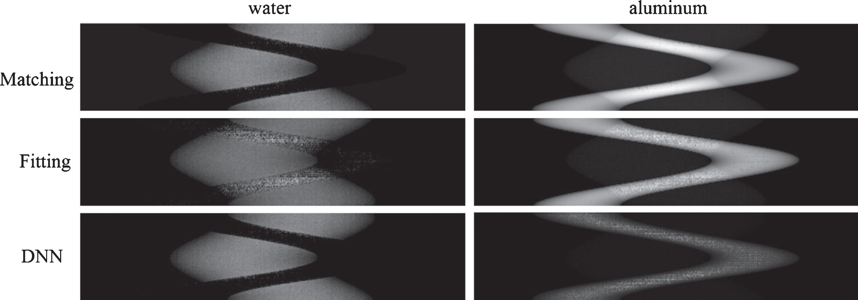
Results of the decomposed projections in real experiment. The size of decomposed projection in real experiment is 360 × 3200. The shape of each image is resized to a proper size for better display.

In the decomposition process, we found that it was difficult for the three methods to fit non-linear transform in the path with low thickness of material. This problem is reflected on the worse performance at the edges of water and aluminum shown in Fig. 11. The fitting method does relatively better at the contact position between two cyclineders. But there also obviously exists many noise points, especially the image of water. DNN generates similar reconstructed images with less noise as the matching method but dos not has the ring artifact caused by beam-harding effect.

Fig.11

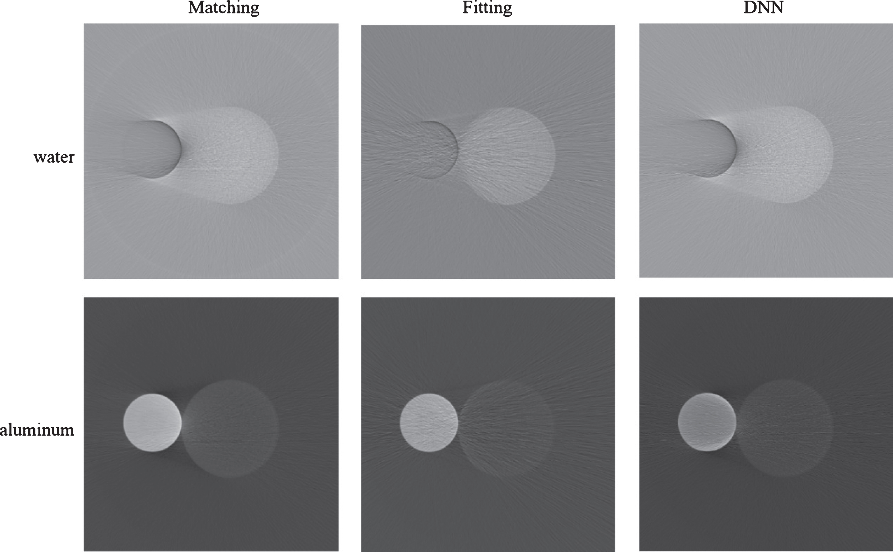
Reconstruction results of real phantom. FBP is used to get the reconstructed images of QRM phantom. The reconstructed material coefficients are also merged into one image. The smaller cylinder is aluminum and the other is water.

Figure 12 plots the horizontal central profile of reconstructed images in Fig. 11. The true CT value of water is 0HU and aluminum is 2150HU. The results of DNN and matching method are close to each other, especially in water curve. The fitting method produces curves with greater fluctuation. This indicates that it is easily affected by photon fluctuation and scattring noise in imaging system. The mainly reason is that the noise may lead to the wrong solution of the fitting equation.

Fig.12

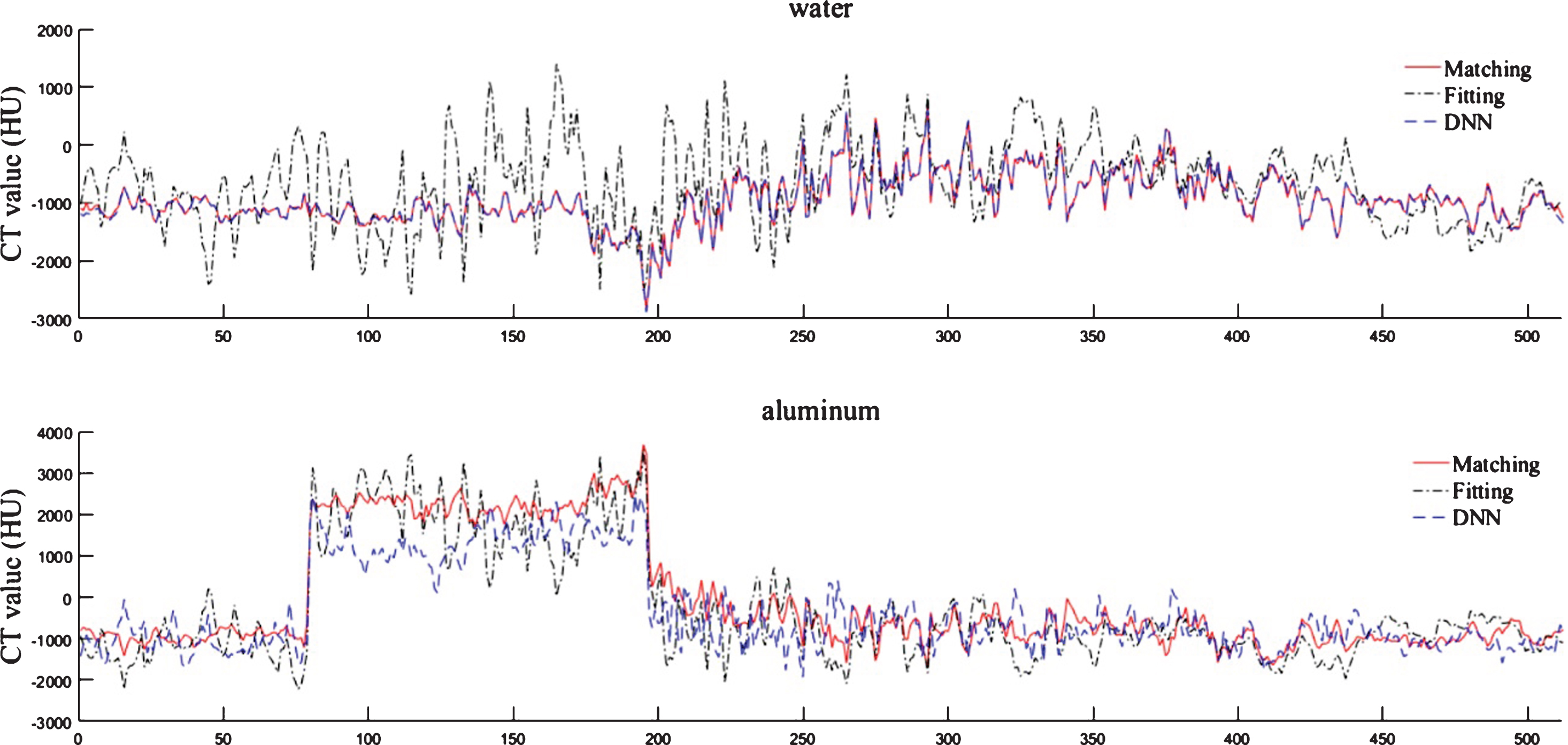
A comparison of central profile of reconstructed images. The Hounsfield unit (HU) values of reconstructed images are calculated. The figure draws the central profile in Fig. 9. The true CT value of water is 0HU and aluminum is 2150HU.

Quantitative evalution of performances on reconstructed images are summarized in Table 7. For the real phantom, we manually sketch out the water and aluminum region on the reconstructed images, to ensure that the metrics are also calculated in ROI. Because the lookup table confines the value of material coefficient to a certain range, the matching method would not give much worse output at some bad points, resulting its better MAD and RMSE. The fitting method has the largest MAD and standard deviation, indicating its sensitive to noises. DNN achieves moderate results and performs best on image quality. Generally, all the methods generate more accurate estimation of aluminum than water. For DNN, this is consistent with the results in the testing dataset, as shown in Fig. 7 (right).

Table 7

A list of quantitative evaluation on reconstructed images in real experiment

Method	water					aluminum
	RMSE (HU)	MAD (HU)	Bias (ratio)	Std (ratio)	PSNR (dB)	RMSE (HU)	MAD (HU)	Bias (ratio)	Std (ratio)	PSNR (dB)
Matching	605.1	1094.1	0.498	0.276	15.43	110.9	570.3	0.356	0.300	23.71
Fitting	589.0	1732.0	0.304	0.440	15.38	202.4	875.6	0.114	0.560	19.33
DNN	598.3	1515.7	0.502	0.359	15.47	297.8	813.7	0.606	0.390	20.47

4 Discussion

The objective of this work is to develop and demonstrate a projection decomposition algorithm based on deep neural network. Two additional decomposition methods are implemented and compared with the proposed network. The experimental results have shown the characteristics of the three methods. For the matching method, the lookup table is a double-edged sword. Its advantage is making the method robust to the photon noise by confining the output value to a certain range and the disadvantages is decreasing the decomposition accuracies. The selection of lookup table needs to balance the precision and speed. Benefiting from the precisely solution of fitting equation, the fitting method achieves high accuracies in simulation and low bias in real experiment. However, it mainly suffers from the noise interferences and higher computational complexity.

The proposed network achieves a comparable performance with significantly fast speed. DNN performs better standard deviation and reconstructed image quality, especially in decomposition test with photon noise. The results in real experiment shown in Figs. 5 and 6 suggest that DNN behaves quit similar as the matching method. The calculation of decomposed images in both methods depends on the same lookup table. The value of parameters in DNN can be regard as a representation of the prior knowledge in lookup table. Compared to other decomposition algorithms based on neural network [13 –15], the proposed algorithm introduces the energy spectrum into the modeling process. The network used in simulation and real experiments is the same one, which proves that it is applicable to different dual energies. The main drawback of DNN is the high bias, which is not consistent with the low bias results in [14]. We hypothesize that this is mainly caused by introduction of energy spectrums. Due to the unexplainable mechanism of deep neural network, it is difficult to understand how DNN works and how to improve the performance of current mode besides increasing more training data. Actually, even though we sampled more training data with low thickness of water or aluminum, the decomposing net still performed worse at the edge of phantom as shown in Fig. 5. In addition, selection of the hyper-parameter in the model is a matter of “trial and error”. Thus, it can be a very time-consuming process to choose the appropriate value of the parameter such as λ in Equation (4).

5 Conclusion and future work

We have developed a projection decomposition algorithm for dual-energy CT via deep neural network. The proposed network features significantly fast speed, low standard deviation and high image quality. It also need not be retrained in the case of different dual energy, thus has extensive application in comparison with other decomposition algorithms based on neural network.

We also recognize two directions of further work that could be done in the future. The first one is the increment learning or online learning of the decomposing net. The second one is the attempt of using convolutional neural network (CNN) to solve the material decomposition problem in image domain, since most current successes obtained by deep neural network in image processing field is contribute to CNN.

Footnotes

Acknowledgments

This work was supported by the national key research and development plan of China under grant 2017YFB1002502 and the National Natural Science Foundation of China (No.61601518 and No.61372172).

References

Ying

, Naidu

and Crawford

C.R.

, Dual energy computed tomography for explosive detection, Journal of X-Ray Science and Technology 14(4) (2006), 235–256.

Vilches-Freixas

, Létang

J.M.

, Ducros

and Rit

, Optimization of dual-energy CT acquisitions for proton therapy using projection-based decomposition, Medical Physics (2017).

Goo

H.W.

and Goo

J.M.

, Dual-energy CT: New horizon in medical imaging, Korean Journal of Radiology 18(4) (2017), 555–569.

Hong

and Chin

T.Y.

, Dual-energy CT in gout-A review of current concepts and applications, Journal of Medical Radiation Sciences 64(1) (2017), 41–51.

, Wang

, Luo

D.H.

et al., Diagnostic value of single-source dual-energy spectral computed tomography for papillary thyroid microcarcinomas, Journal of X-ray Sciece and Techology 25(5) (2017), 793–802.

Stenner

, Berkus

and Kachelriess

, Empirical dual energy calibration (EDEC) for cone-beam computed tomography, Medical Physics 34(9) (2007), 3630–3641.

Shen

, Xing

, Zhang

et al., Hybrid decomposition method for dual energy CT, Nuclear Science Symposium and Medical Imaging Conference, 2016, pp. 1–4.

Zhao

, Li

and Chen

, K-edge eliminated material decomposition method for dual-energy X-ray CT, Appl Radiat Isot 127 (2017), 231–236.

Brendel

and Schlomka

J.P.

, Empirical projection-based basis-component decomposition method, Proceedings of SPIE-The International Society for Optical Engineering 7258 (2009), 72583Y–72588Y-8.

10.

Jaccard

, Rogers

T.W.

, Morton

E.J.

and Griffin

L.D.

, Detection of concealed cars in complex cargo X-ray imagery using deep learning, Journal of X-ray Science and Technology 25(3) (2017), 323–339.

11.

Sun

, Zheng

and Qian

, Automatic feature learning using multichannel ROI based on deep structured algorithms for computerized lung cancer diagnosis, Computers in Biology and Medicine 89 (2017), 530–539.

12.

Wang

, A perspective on deep imaging, IEEE Access 4(99) (2016), 8914–8924.

13.

Schmidt

T.G.

and Zimmerman

K.C.

, Material Decomposition of Multi-spectral X-Ray Projections Using Neural Networks, US Patent, US20150371378, 2015.

14.

Zimmerman

K.C.

and Schmidt

T.G.

, Experimental comparison of empirical material decomposition methods for spectral CT, Physics in Medicine & Biology 60(8) (2015), 3175–3191.

15.

Lee

W.J.

, Kim

D.S.

, S.W. et al., Material depth reconstruction method of multi-energy X-ray images using neural network, International Conference of the IEEE Engineering in Medicine and Biology Society, 2012, pp. 1514–1517.

16.

Bengio

, Lamblin

, Popovici

and Larochelle

, Greedy layer-wise training of deep networks, Advances in Neural Information Processing Systems 19 (2007), 153–160.

17.

Hinton

, Osindero

and Teh

Y.W.

, A fast learning algorithm for deep belief nets, Neural Computation 18(7) (2014), 1527–1554.

18.

Salakhutdinov

and Hinton

, Deep boltzmann machines, Journal of Machine Learning Research 5(2) (2009), 1967–2006.

19.

Denton

, Gross

and Fergus

, Semi-Supervised Learning with Context-Conditional Generative Adversarial Networks, 2016.

20.

Bengio

, Goodfellow

I.J.

and Courville

, Deep Learning, Book in preparation for MIT Press (2016). http://www.deeplearningbook.org.

21.

Rumelhart

D.E.

, Hinton

G.E.

and Williams

R.J.

, Learning representations by back-propagating errors, Nature 323 (1986), 533–536.

22.

Poludniowski

, Landry

, Deblois

et al., SpekCalc: A program to calculate photon spectra from tungsten anode x-ray tubes, Physics in Medicine & Biology 54(19) (2009), N433–N438.

23.

Seltzer

S.M.

, XCOM: Photon Cross Sections Database, 2005.

24.

, Wang

, Cai

et al., Projection decomposition algorithm for X-ray dual-energy computed tomography based on isotransmission line fitting, Acta Optica Sinica 36(8) (2016), 0834001.

25.

and Zhang

, Projection decomposition algorithm of X-ray dual-energy computed tomography based on projection matching, Acta Optica Sinica 31(3) (2011), 82–87.

26.

, Christner

J.A.

, Leng

et al., Virtual monochromatic imaging in dual-source dual-energy CT: Radiation dose and image quality, Medical Physics 38(12) (2011), 6371–6379.