Structure tensor total variation for CBCT reconstruction

Abstract

The total variation (TV) regularization has been widely used in statistically iterative cone-beam computed tomography (CBCT) reconstruction, showing ability to preserve object edges. However, the TV regularization can also produce staircase effect and tend to over-smooth the reconstructed images due to its piecewise constant assumption. In this study, we proposed to use the structure tensor total variation (STV) that penalizes the eigenvalues of the structure tensor for CBCT reconstruction. The STV penalty extends the TV penalty, with many important properties maintained such as convexity and rotation and translation invariance. The STV penalty utilizes gradient information more effectively and has a stronger ability to capture local image structural variation. The objective function was constructed with the penalized weighted least-square (PWLS) strategy and the gradient descent (GD) method was used to optimize the objective function. Besides, we investigated whether the norms involved in the STV penalty affected the reconstruction performance and found that the l₁-norm gave the better performance than the l₂-norm and l_∞-norm. We also examined performance of the STV penalties constructed using different kernel functions and found that the STV with the Gaussian kernel had the best performance, and the STVs with Uniform, Logistic, and Sigmoid kernels had similar performance to each other. We evaluated our reconstruction method with the STV penalty on computer simulated phantoms and physical phantoms. The results demonstrated that STV led to better reconstruction performance than TV, both visually and quantitatively. For the Catphan 600 physical phantom, the STV₁ penalty was 175% and 623% better than the low-dose FDK and the high-dose FDK, and 14% better than the TV penalty at the matched noise level, according to the average contrast-to-noise ratio (CNR); while for the Compressed Sensing simulation phantom, the peak signal to noise ratio (PSNR) of reconstructed results using STV₁, STV₂, and STV_∞ were 40.67 dB, 38.72 dB, and 37.40 dB, respectively, all being significantly better than 36.84 dB using TV.

Keywords

CBCT structure tensor total variation image reconstruction staircase effect

1 Introduction

Cone-beam computed tomography (CBCT) has already been increasingly used in image guided radiation therapy [1] to obtain patients’ updated anatomy at the treatment position. However, overuse of the CBCT imaging during a course of radiotherapy treatment may bring excessive X-ray radiation to patients [2, 3]. Using lower mAs scan protocols in CBCT projection is a widely used method to reduce the radiation dose [4]. However, it degrades the quality of the reconstruction image [5, 6] because of the increasing noise level. Low dose CBCT reconstruction with better image quality is highly desired in the clinic.

CBCT image reconstruction algorithms include analytic reconstruction methods and iterative reconstruction methods. In the development of the analytical algorithms, Tuy first proposed a practical cone-beam inverse transformation formula, which established the mathematical connections between the projection data and the reconstructed image [7]. Feldkamp et al. proposed the FDK algorithm to approximate the three-dimensional image reconstruction in 1984 [8]. In 1991, Grangeat proposed the Grangeat reconstruction algorithm based on the circular scan trajectory [9]. In 2001, Katsevich proposed a reconstruction algorithm that was easy to implement based on the helical scan trajectory [10]. Among them, the FDK algorithm has been the mainstream in practical applications. This algorithm is simple and computationally efficient, but vulnerable to noise and easy to produce artifacts.

Iterative reconstruction methods include non-statistical iterative reconstruction methods and statistical iterative reconstruction (SIR) methods. Non-statistical iterative methods, such as the algebraic reconstruction technique (ART) [11], achieves image reconstruction by solving a system of linear equations, which can give fairly accurate solutions once these equations are compatible. However, in practice, because of the existence of noise, these equations are always not compatible, so the solutions obtained by such method are rather unstable.

In statistical iterative algorithms, the objective functions are constructed using noise statistical characteristics and the prior knowledge, based on the Bayesian theory [12]. An objective function includes a term that is called the penalty term reflecting the prior constraint on the solutions. The penalty term affects the quality of the reconstruction results greatly. Some commonly used penalty terms are the isotropic quadratic penalty [13], Huber penalty [14], total variation (TV) penalty [15, 16], and so on. SIR algorithms based on the prior information have been widely utilized for low-dose CBCT imaging [17, 18]. The quality of the obtained image by SIR is generally superior to that of the FDK method, with much less artifacts and lower noise.

The TV penalty has great popularity in various image-related inverse problem, thanks to its great performance in both suppressing noise and preserving edges. However, the TV regularization sometimes produces the staircase effect and tend to over-smooth the image due to its piecewise constant assumption [19, 20]. To avoid the staircase effect, several penalties have been proposed, such as ATV [21], TGV [22], NLTV [23], and Hessian [24, 25].

In this article, we introduced the structure tensor total variation (STV) that penalizes the eigenvalues of the structure tensor into the objective function to utilize the gradient information more effectively for CBCT reconstruction. The STV penalty extends the TV penalty, with many important properties maintained like convexity and rotation and translation invariance [26]. The STV penalty has a stronger ability in capturing the structural variation among local areas, leading to reconstruction of a high quality. We constructed the objective function with the penalized weighted least-square (PWLS) and employed the gradient descent (GD) method for the associated optimization problem. We evaluated the proposed statistical reconstruction method with the STV penalty on computer simulated phantoms and physical phantoms. The results demonstrated the outstanding ability of the STV penalty over the TV penalty.

2 Mathemtical models

2.1 PWLS Image Reconstruction

Assuming that the incident photon number of the X-ray is I_o, and the detected photon number is I_d. According to the Beer law [2], we can get the relation between the incident and detected photon number:

$\frac{I_{d}}{I_{o}} = exp (- \hat{y}),$ (1) where $\hat{y}$ denotes the line integral along the X-ray path l of the tissue attenuation, i.e. $\hat{y}$ is the projection. Thus, we can get the following expression: $\hat{y} = ln \frac{I_{o}}{I_{d}} = \int_{l} u (x, y, z) dl,$ (2) where u represents the linear attenuation coefficient (the image to be reconstructed). The noise distribution of the projection data can be well approximated using Gaussian [18]. As a result, the variance $σ_{i}^{2}$ of the projection y_i at the ith detector bin can be calculated as [2]: $σ_{i}^{2} = exp ({\bar{y}}_{i}) / - I_{i 0},$ (3) where I_i0 is the emitted photon numbers, and ${\bar{y}}_{i}$ is the mean value of the detected projection data, both at the ith detector bin. The probability density function of the projection data conditioned on the attenuation coefficient is [18] $prob (y_{i} | u) = \prod_{i} \frac{1}{\sqrt{2 π} σ_{i}} exp (- \frac{{(A_{i} u - y_{i})}^{2}}{2 σ_{i}^{2}}),$ (4) where A_i represents the ith row of the projection matrix A.

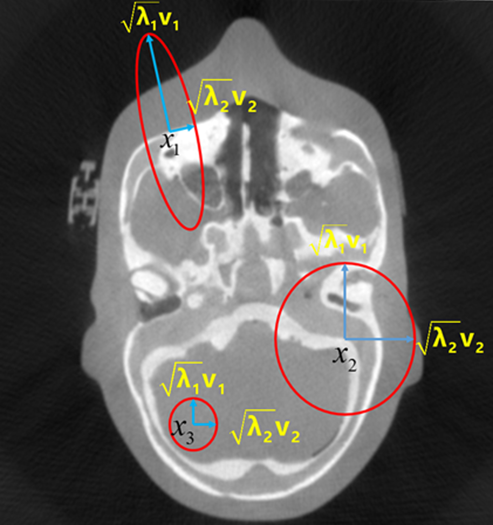
Taking a logarithm transform over (4) and using the maximum a posteriori estimate, we can get the objective function for CBCT reconstruction [4]: $Φ (u) = \frac{1}{2} {(y - Au)}^{T} Σ^{- 1} (y - Au) + τ R (u),$ (5) where Σ is a diagonal matrix with its ith element $σ_{i}^{2}$ , symbol T denotes the transpose operator. The first term in the right hand side of (5) is referred to as the weighted least-squares (WLS) criterion or the fidelity term evaluating the consistency between the log-transformed measured projection data y and the theoretical value Au. The second term in the right hand side of (5), called the penalty term, provides constraints on the solution of the objective function. τ ⩾ 0 is a tradeoff regularization parameter balancing the contribution of the fidelity term and the penalty term to the whole objective energy. CBCT reconstruction is modelled as minimizing the objective functional (5).

2.2 Structure tensor

The structure tensor [26], the most common tensor, is defined as the spatial average of the outer product of the gradient with itself at point x of the image (the attenuation coefficients) u: $S_{g} u (x) = g * (\nabla u (x)) {(\nabla u (x))}^{T} = g * [\begin{matrix} u_{x}^{2} (x) u_{x} (x) u_{y} (x) \\ u_{x} (x) u_{y} (x) u_{y}^{2} (x) \end{matrix}],$ (6) where ∇ is the gradient operator, g is a nonnegative, rotationally symmetric convolution kernel, i.e.,g (x) = g (|x|). Any nonnegative, rotationally symmetric convolution kernel g can be used to define the structure tensor in Equation (6). The convolution kernel can reduce the influence of noise on the derivative operation and improve the robustness of gradient information extraction. The Gaussian kernel is the most popular one used to design the structure tensor [26]. The 1D normalized version of those used kernels in our study can be described as follows:

Gaussian kernel: $g (x) = \frac{1}{\sqrt{2 π}} e^{- \frac{1}{2} x^{2}};$ Uniform kernel: $g (x) = \frac{1}{2}, | x | ⩽ 1;$

Logistic Kernel: $g (x) = \frac{1}{e^{x} + 2 + e^{- x}};$ Sigmoid Kernel: $g (x) = \frac{2}{π} \frac{1}{e^{x} + e^{- x}}$ .

Let λ_i be the eigenvalues of the structure tensor S_gu (x), ordered so that λ₁ ⩾ λ₂, and v_i are the corresponding unit eigenvectors. Compared with the gradient, the eigenvalues of the structure tensor can reflect richer local structure information of an image, thanks to the outer product and convolution operation. Figure 1 shows the structure tensors at three voxels, x₁, x₂, and x_3, respectively, together with their associated unit eigenvectors v₁, v₂ and rooted eigenvalues $\sqrt{λ_{1}}$ , $\sqrt{λ_{2}}$ . Each structure tensor in Fig. 1 can be denoted as an ellipses, with its major radius and direction given by the rooted eigenvalue $\sqrt{λ_{1}}$ and the eigenvector v₁, respectively, and the minor radius and direction determined by $\sqrt{λ_{2}}$ and v₂, respectively. The rooted eigenvalues quantitatively reflect the degree of image intensity change, while their related eigenvectors reflect the change direction. Thus, the directional variation of a specific point in the image can be explained as point-to-center distance along the ellipse.

Fig.1

Structure Tensor.

For a given point x in the image, when both the eigenvalues λ₁ and λ₂ of the structure tensor are small, the intensity change in any direction near this point is small. In other words, the local neighborhood centered on x tends to be smooth. When λ₁ is large and λ₂ is small, the image intensity in the local neighborhood varies greatly in one direction, indicating the existence of obvious edge structure characteristics. When both λ₁ and λ₂ are large, the image intensity changes quickly in all directions, suggesting that the current point is an image corner.

2.3 Vector p norm penalty

The TV penalty [27] has demonstrated state-of-the-art performance in preserving edges of the reconstructed image, and is defined as: $R_{TV} (u) = \sum_{x, y, z} \sqrt{u_{x}^{2} (x, y, z) + u_{y}^{2} (x, y, z) + u_{z}^{2} (x, y, z)} .$ (7)

In this study, to design regularization terms that integrate the local image intensity variation around each pixel, we constructed penalties using a combination of eigenvalues of the structure tensor, as follows [26]: ${STV}_{p} (u) = \sum_{n = 1}^{N} {∥ (\sqrt{{(λ_{1})}_{n}}, \sqrt{{(λ_{2})}_{n}}) ∥}_{p},$ (8) where p ⩾ 1, ∥ • ∥ _p is the vector norm of order p.

The STV generalizes several existing image regularization methods. Specifically, noting that when g (x) is the Dirac delta δ (x), all the penalties with different orders are equal to TV. The STV provides more robust and coherent measures of an image than TV, as these measures include the intensity variations in all directions over the local neighborhood. In this way, STV is in general more suitable for describing the local image geometry and leads to better results in CBCT reconstruction.

It was shown that the STV penalties maintain many favorable properties of TV, i.e. translation and rotation invariant, 1-homogeneous, and convex [26].

2.4 Details in calculating the projection matrix A

The difficulty in the calculation of the projection matrix A is that it is too enormous to store. So, a proper algorithm to calculate A effectively is essential. The Siddon’s algorithm [28] is widely used to calculate the projection matrix A for its simplicity in calculation. In this work we adopted the separable footprint (SF) [29] algorithm to calculate matrix A, which is faster than the Siddon’s algorithm. We calculated the entries of the matrix A whenever we need it rather than storing it.

3 Minimization of objective function

3.1 Objective Function in CBCT Reconstruction

Employing the STV penalties (8) in the objective function (5), we can obtain: $\begin{matrix} Φ (u) = \frac{1}{2} {(y - Au)}^{T} Σ^{- 1} (y - Au) + τ {STV}_{p}, \\ = \frac{1}{2} {(y - Au)}^{T} Σ^{- 1} (y - Au) + τ \sum_{n = 1}^{N} {∥ (\sqrt{{(λ_{1})}_{n}}, \sqrt{{(λ_{2})}_{n}}) ∥}_{p} . \end{matrix}$ (9)

Hence, the CBCT reconstruction becomes a minimization problem of the objective function (9) and we tested three cases with p = 1, 2, ∞ in this study.

3.2 Gradient descent method

Lefkimmiatis et al. used the STV penalty for nature image denoising and deblur, and proposed to optimize the corresponding objective function through a patch-based Jacobian operator [26]. The optimization algorithm they employed combined the majorization-minmization (MM) [30] method, MFISTA [31] method and primal-dual [32] method.

We note that the algorithm used by Lefkimmiatis et al. in [26] is computationally expensive for CBCT reconstruction in practice. To optimize the objective function (9) with a simpler and faster method, we intended to calculate its gradient firstly. The most intractable part in the gradient calculation of the objective function (9) came from the STV penalty. Consider the following functional:

$R (u) = \int_{Ω} φ (λ_{1}, λ_{2}) d x,$ (10) where Ω ∈ R², φ (λ₁, λ₂) : (R⁺) ² → R⁺ is a cost function, with two independent variables: λ₁ and λ₂ (the two eigenvalues of the structure tensor S_gu (x)). Compared to the traditional variational methods, the difficulty of this problem is that it does not depend on the derivative of the image, but the product involved with the convolution kernel operation. Roussos and Maragos [33] showed that the gradient of functional (10) w.r.t the image u (x) is: $\frac{\partial R (u)}{\partial u} = - div (D_{g} \nabla u),$ (11) where $D_{g} = g * (2 \sum_{i} \frac{\partial φ}{\partial λ_{i}} v_{i} \otimes v_{i})$ [33].

Applying (11) to CBCT reconstruction, we could calculate the gradient of the objective function (9) as follows: $\nabla Φ (u) = A^{T} Σ^{- 1} (Au - y) - τ div (D_{g} \nabla u),$ (12) where D_g depends on the order p. We have the following three cases:

Case 1. For p = 1, i.e. ${STV}_{1} (u) = \sum_{n = 1}^{N} (\sqrt{{(λ_{1})}_{n}} + \sqrt{{(λ_{2})}_{n}}), D_{g} = g * (\sum_{i} \frac{1}{\sqrt{λ_{i}}} v_{i} \otimes v_{i}) .$

Case 2. For p = 2, i.e. ${STV}_{2} (u) = \sum_{n = 1}^{N} (\sqrt{{(λ_{1})}_{n} + {(λ_{2})}_{n}}), D_{g} = g * (\sum_{i} \frac{1}{\sqrt{λ_{1} + λ_{2}}} v_{i} \otimes v_{i}) .$

Case 3. For p =∞, i.e. ${STV}_{\infty} (u) = \sum_{n = 1}^{N} (\sqrt{{(λ_{1})}_{n}}), D_{g} = g * (\frac{1}{\sqrt{λ_{1}}} v_{1} \otimes v_{1}) .$

Given the gradient in Equation (12), we could optimize the objective functional (9) with the gradient descent (GD) method directly. Our proposed algorithm for CBCT reconstruction using STV are summarized as follows.

Algorithm: CBCT Reconstruction Using STV

Input:y, A, τ, Σ, g, α

Initialization:k = 1, u₀ = FDK(y), M = 100.

Whilek < M and

{∥ u_{k} - u_{k - 1} ∥}_{2}^{2} / {∥ u_{k - 1} ∥}_{2}^{2} < 1 \times 10^{- 5}

| \begin{array}{l} \nabla Φ (u_{k - 1}) = A^{T} \sum^{- 1} (A u_{k - 1} - y) - τ div (D_{g} \nabla u_{k - 1}); u_{k} = u_{k - 1} - α \cdot \nabla Φ (u_{k - 1}); \\ k = k + 1; \end{array}

u_k = u_k-1 - α · ∇ Φ (u_k-1);

k = k + 1 ;

end

Returnu.

For the convenience of the readers, we summarize the notations used in the Algorithm below.

y: projection data;

A: projection (system) matrix;

τ: positive regularization parameter (τ > 0);

Σ: diagonal noise covariance matrix;

g: kernel with a specific size and shape;

α: step length determined by backtracking one-dimensional search method;

M: maximum iteration number.

Note that we took the FDK reconstruction to initialize u, namely, u₀ = FDK(y).

4 Materials and evaluation

We evaluated our methods on two simulated phantoms and two physical phantoms. For CBCT reconstruction, the regularization parameter τ in Equation (5) always plays a role to balance the image resolution and noise level. To have a reasonable comparison of the performance of different penalties, we adjusted this parameter for each phantom to keep all the reconstruction results to have a similar noise level [24, 34].

4.1 Simulated Phantom

The two computer simulation phantoms were the Compressed Sensing (CS) phantom and a modified Shepp-Logan phantom, respectively. Figure 2(a) and Fig. 4(a) show one representative slice of the CS phantom and the Shepp-Logan phantom, respectively. The CS phantom has 350×350×16 pixels, and the physical size of each pixel is 0.776×0.776×0.776 mm³. The projection of the CS phantom covers 360 angles, with each angle having 800×200 pixels. The Shepp-Logan phantom has 350×350×16 pixels, and the voxel size is 0.776×0.776×0.776 mm³. The projection of Shepp-Logan phantom covers 360 angles and have 500×500 pixels for each angle. The source-to-axial distance is 100 cm and the source-to-detector is 150 cm for both CS phantom and Sheep-Logan phantom. Note that most of commercial CBCT systems for image-guided radiation therapy use such a geometry design. For each phantom, the incident photon number in (3) was set to be 1×10⁴ to simulate the low dose case and the Gaussian noise according to the model (3) was added to the projection data.

Fig.2

A representative slice of the CS phantom using different penalties.

Fig.3

SSIM map of the CS phantom using different penalties.

Fig.4

A representative slice of the Shepp-Logan phantom using different penalties.

4.2 Physical phantom

The commercial calibration phantom CatPhan 600 (The Phantom Laboratory, Inc., Salem, NY) and the anthropomorphic head phantom were tested in our experiment, respectively. Figure 6(a) and Fig. 7(b) demonstrate one typical slice of the CatPhan 600 phantom and the anthropomorphic head phantom, respectively. The CatPhan 600 phantom covers 350×350×16 pixels, with each pixel having a physical size of 0.776×0.776×0.776 mm³. The projection of the CatPhan 600 phantom covers 634 angles and each angle has 1024×768 pixels. The anthropomorphic head phantom covers 550×550×32 pixels, and each pixel has a physical size of 0.338×0.338×0.338 mm³. The projection of the anthropomorphic head phantom has 1024×768 pixels and covers 678 angles. The source-to-axial distance is 100 cm and the source-to-detector distance is 150 cm for both phantoms. For each phantom, the tube voltage was 125 kVp and the tube current was 10 mA (low dose) and 80 mA (high dose), respectively, lasting for 10 ms at each projection scan.

Fig.5

Profiles through the ellipsoid object in Figure 4(a).

Fig.6

A representative slice of the Catphan 600 phantom using different penalties.

Fig.7

A representative slice of the head phantom using different penalties.

4.3 Evaluation

In this study, we adopted the peak signal to noise ratio (PSNR), the improvement signal to noise ratio (ISNR), the contrast-to-noise ratio (CNR), and the structural similarity (SSIM) indexes for evaluation [24].

PSNR is defined as $PSNR = 10 {log}_{10} (\frac{μ_{max}^{2}}{MSE}),$ (13) where μ_max is the maximum possible value of the image and MSE is the mean-squared error between the reconstructed image and the reference image. A higher PSNR means less error between the reconstructed image and the reference image.

ISNR is defined as $ISNR = 10 {log}_{10} (\frac{{MSE}_{in}}{{MSE}_{out}}),$ (14) where MSE_in is the mean-square error between the reconstructed image and the reference image and MSE_out between the FDK image and the reference image. A higher ISNR means higher quality of the reconstructed image compared with the FDK image.

CNR is defined as $CNR = \frac{| μ_{ROI} - μ_{Ref} |}{\sqrt{σ_{ROI}^{2} + σ_{R ef}^{2}}},$ (15) where μ_ROI and μ_Ref are the mean intensity of the ROI and the background region, respectively, and σ_ROI and σ_Ref are the standard deviation of the ROI and the background region, respectively. A higher CNR means better preservation of the image contrast.

SSIM is defined as $SSIM (a, b) = \frac{(2 μ_{a} μ_{b} + C_{1}) (2 λ_{ab} + C_{2})}{(μ_{a}^{2} + μ_{b}^{2} + C_{1}) (λ_{a}^{2} + λ_{b}^{2} + C_{2})},$ (16) where a and b are two windows of 11 × 11 pixels in the same position in two images, μ_a, μ_b and $λ_{a}^{2}, λ_{b}^{2}$ are their intensity means and variances, respectively, λ_ab are the intensity covariance between the two windows, and C₁ = (0.01μ_max) ² and C₂ = (0.03μ_max) ² are chosen to avoid instability. A higher SSIM means that the regions in the two windows are more similar.

5 Experimental results

5.1 CS Phantom

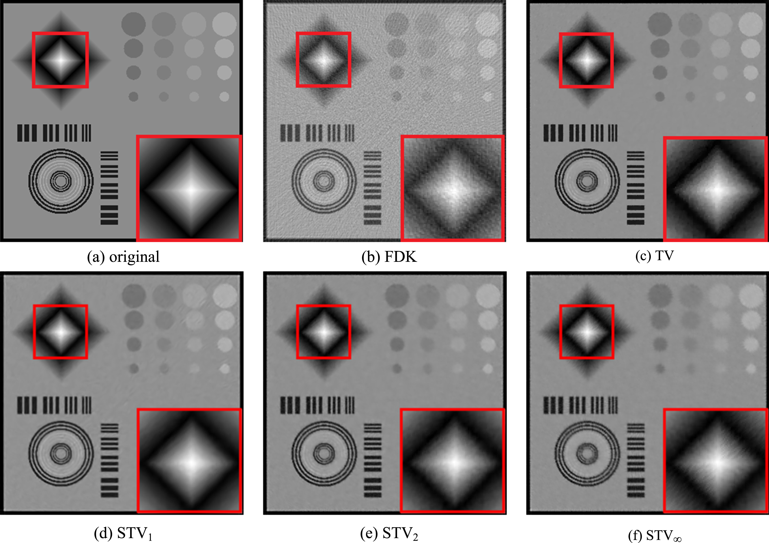
Figure 2 shows a typical slice of the images of the CS phantom reconstructed by different penalties. Figure 2(a) shows the original image, and Fig. 2(b) shows the FDK reconstruction image. Figure 2(c-f) show the reconstruction images by the TV penalty, the STV₁ penalty (p = 1), the STV₂ penalty (p = 2), and the STV_∞ penalty (p =∞), respectively. The smaller red rectangle in Fig. 2(a) denotes the ROI, enlarged and displayed in the lower right corner of Fig. 2(a) (same for Figs. 2(b-f)). Figure 2 indicates that the reconstruction images using the TV penalty produced piecewise-constant regions obviously, while all the three STV penalties could avoid the staircase effect effectively.

Table 1 lists the values of PSNR, ISNR, mean SSIM (the average SSIM values) of the ROI in Fig. 1(a) with different penalties. The quality of the reconstruction results by the three STV penalties were better than TV according to these three indexes. Among the three STV penalties, the STV₁ had the best evaluation indexes.

Table 1
The evaluation indexes of the reconstruction of CS phantom using different penalties

Penalty Noise (×10^-4) PSNR(dB) ISNR(dB) Mean SSIM

TV 1.2925 36.8412 7.1799 0.9492

STV₁ 1.2618 40.6858 11.0245 0.9786

STV₂ 1.2766 38.7155 9.0542 0.9669

STV_∞ 1.3030 37.3958 7.7345 0.9539

Penalty	Noise (×10^-4)	PSNR(dB)	ISNR(dB)	Mean SSIM
TV	1.2925	36.8412	7.1799	0.9492
STV₁	1.2618	40.6858	11.0245	0.9786
STV₂	1.2766	38.7155	9.0542	0.9669
STV_∞	1.3030	37.3958	7.7345	0.9539

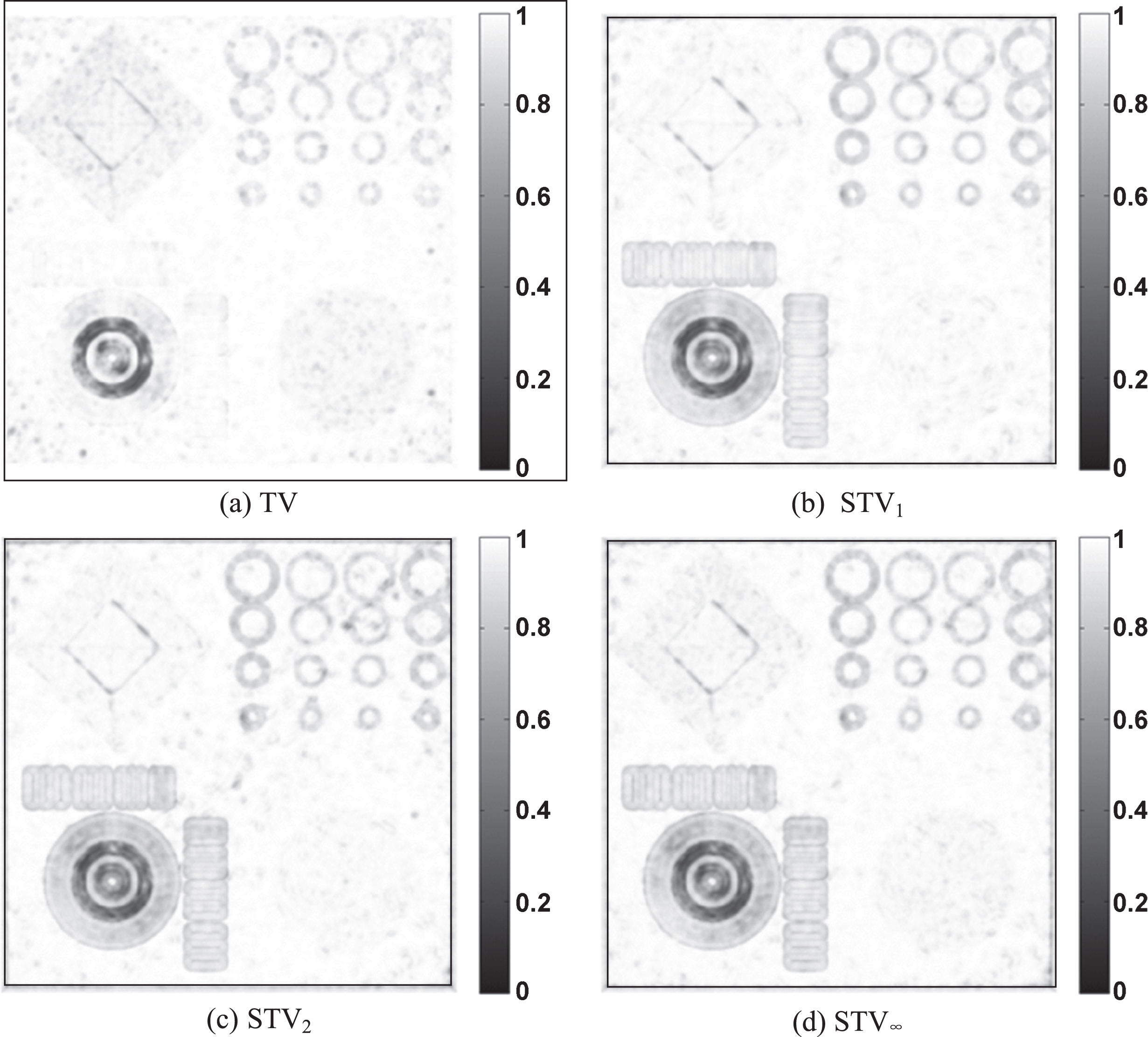
Figure 3 shows the SSIM map of the reconstructed image using different penalties over the original image. In the octahedral region (the upper left part), the reconstruction images by the STV penalties have higher SSIM values (whiter) than that those of the TV penalty, indicating a better preserving of regions with smooth intensity transition. However, at the barcode areas (the lower left part), the TV penalty had higher SSIM values, indicating a better ability in preserving sharp edges.

Table 2 lists the values of PSNR, ISNR, mean SSIM of the ROI in Fig. 1(a) using the STV₁ penalty with different Gaussian kernels. As we can see, the reconstructed performance of the STV penalty varied with the size and shape of the used kernel. A too sharp kernel leaded a low reconstruction quality such as those in Table 2 with variance 0.5 and 1, respectively. In Table 2, the Gaussian kernel with size 7×7 and variance 2 had the best performance.

Table 2

The evaluation indexes of the reconstruction of CS phantom using STV₁ with different Gaussian kernels

Size	Variance	Noise (×10^-4)	PSNR(dB)	ISNR(dB)	mean SSIM
11×11	2	1.2604	40.1218	10.4605	0.9765
11×11	1	1.2608	39.9099	10.2486	0.9745
11×11	0.5	1.2604	39.0985	9.4372	0.9686
9×9	2	1.2601	40.5528	10.8915	0.9781
9×9	1	1.2603	39.8907	10.2294	0.9744
9×9	0.5	1.2610	38.7258	9.0645	0.9663
7×7	2	1.2618	40.6858	11.0245	0.9786
7×7	1	1.2663	40.2846	10.6233	0.9766
7×7	0.5	1.2605	39.0985	9.4372	0.9686
3×3	2	1.2617	39.9669	10.3055	0.9744
3×3	1	1.2606	39.3136	9.6523	0.9709
3×3	0.5	1.2700	39.1984	9.5371	0.9692

It is also interesting to see how other types of kernels other than Gaussian kernels perform in CBCT reconstruction when using STV penalties. For comparison, we also used the Uniform kernel, the Logistic kernel, and the Sigmoid kernel to construct the STV₁ penalty.

Table 3 lists the values of PSNR, ISNR, mean SSIM of the ROI in Fig. 1(a) using STV₁ penalties with different types of kernels, all with size 7×7. As we can see, the Gaussian kernel (with variance 2) had the best performance, while the other three types of kernels had similar performance (but all were worse than Gaussian). If not specified, we used Gaussian kernel to construct the STV penalties elsewhere for experiments in this study.

Table 3

The evaluation indexes of the reconstruction of CS phantom using STV₁ with different kernels

Kernel	Noise (×10^-4)	PSNR(dB)	ISNR(dB)	mean SSIM
Gaussian	1.2618	40.6858	11.0245	0.9786
Uniform	1.2622	40.0088	10.3475	0.9760
Logistic	1.2602	40.0188	10.3574	0.9759
Sigmoid	1.2604	40.0198	10.3585	0.9759

5.2 3D Shepp-Logan Phantom

Figure 4 displays a typical slice of the reconstructed images by different penalties for the modified Shepp-Logan phantom. Figure 4(a) displays the original image, and Fig. 4(b) displays the FDK reconstruction image. Figure 4(c-f) displays the reconstruction image by the TV penalty, the STV₁ penalty, the STV₂ penalty and the STV_∞ penalty, respectively. The smaller blue rectangle in Fig. 4(a) denotes the ROI, enlarged and displayed in the lower right corner of Fig. 4(a) (same for Figs. 4(b-f)). Figure 4 indicates that the reconstruction images using the STV penalties are all smoother than the reconstruction image using the TV penalty. Note that TV leaded to significant staircase effect.

Figure 5 shows the intensity profiles along the red line (shown in Fig. 4(a)) through the ellipsoid of the reconstruction images. These profiles show that the reconstruction image using the TV penalty produced piecewise-constant regions, while the reconstructed images using the STV penalties were smoother than the TV result.

5.3 Catphan 600 Phantom

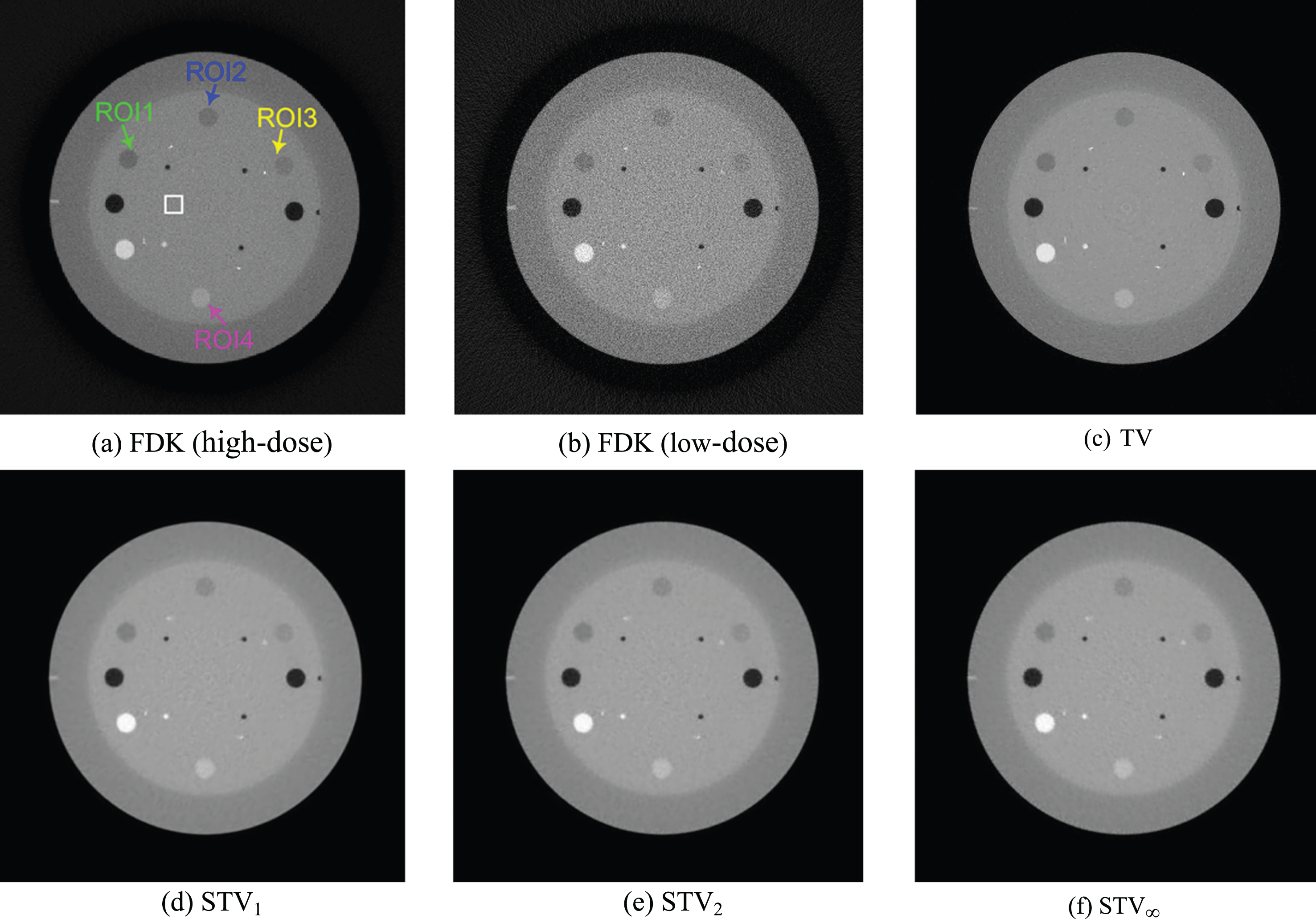
Figure 6 shows a slice of the reconstruction results obtained by different penalties for the Catphan 600 phantom. Figure 6(a) shows the reconstruction image by FDK with a high-dose protocol (80 mA/10 ms). Figure 6(b) shows the reconstruction image by FDK with a low-dose protocol (10 mA/10 ms). Figure 6(c-f) shows the low-dose reconstruction image by the TV penalty, the STV₁ penalty, the STV₂ penalty, and the STV_∞ penalty, respectively. The white rectangle in Fig. 6(a) denotes the region to be used to calculate noise level. Figure 6 indicates that the reconstruction images using the TV and STV penalties all have a good ability in suppressing noise.

Furthermore, we chose four ROIs indicated by arrows in Fig. 6(a) to calculate CNR for a quantitative comparison. Table 4 listed the CNR of the four different regions with different penalties for low-dose reconstruction. As we can see, in most cases the STV results have higher CNR values than those from the TV results and both the high-dose and low-dose FDK results, indicating that the STV penalties had a good ability in preserving the contrast of the objects. At the same time, the STV₁ penalty has higher CNR values than those of the STV₂ and STV_∞ penalties. Particularly, when averaged on the four ROIs, the improvement of the CNR of the STV₁ penalty over the TV penalty, the low-dose FDK and the high-dose FDK is 14%, 175%, and 623%, respectively.

Table 4
CNRs of different ROIs in Fig. 4(a)

Penalty Noise (×10^-4) ROI1 ROI2 ROI3 ROI4 Average

FDK(80 mA) 8.6186 3.5817 2.5815 2.0202 2.5141 2.6743

FDK(10 mA) 24 1.4686 0.9216 0.7801 0.9045 1.0187

TV 3.6440 8.6106 5.7256 5.1350 6.2904 6.4404

STV₁ 3.5360 11.5912 6.2735 5.5239 6.0883 7.3692

STV₂ 3.6882 10.8864 5.9039 5.2486 5.9039 6.9857

STV_∞ 3.5489 10.7365 5.6589 5.3591 6.0058 6.9401

Penalty	Noise (×10^-4)	ROI1	ROI2	ROI3	ROI4	Average
FDK(80 mA)	8.6186	3.5817	2.5815	2.0202	2.5141	2.6743
FDK(10 mA)	24	1.4686	0.9216	0.7801	0.9045	1.0187
TV	3.6440	8.6106	5.7256	5.1350	6.2904	6.4404
STV₁	3.5360	11.5912	6.2735	5.5239	6.0883	7.3692
STV₂	3.6882	10.8864	5.9039	5.2486	5.9039	6.9857
STV_∞	3.5489	10.7365	5.6589	5.3591	6.0058	6.9401

5.4 Anthropomorphic head phantom

Figure 7 shows a slice of the reconstruction results obtained by different penalties for the head phantom. Figure 7(a) and (b) display the reconstruction images by FDK with the high-dose protocol (80 mA/10 ms), and the low-dose protocol (10 mA/10 ms), respectively. Figure 7(c-f) display the low-dose reconstruction image by the TV penalty, the STV₁ penalty, the STV₂ penalty, and by the STV_∞ penalty, respectively. The blue rectangle in Fig. 7(a) denotes the region to be used to calculate the noise level.

The ROI is indicated by the red rectangle in Fig. 7(a) to calculate SSIM. We can see in Fig. 8 that the mean SSIM of those STV penalties are higher than that of the TV penalty, indicating that the STV penalties have a better ability in preserving regions with gradual intensity transitions than the TV penalty. The STV₁ penalty had the best mean SSIM of the reconstructions result.

Fig.8

SSIM maps of the Anthropomorphic head phantom using different penalties.

6 Discussion and conclusion

In the study, we proposed to use the STV penalty for statistical iterative CBCT reconstruction based on the PWLS criteria. Experimental results suggested that the STV penalty can significantly suppress the staircase effect, and had better reconstruction performance than the TV penalty. Among the orders 1, 2 and ∞, the STV₁ penalty constructed using norm with order 1 (i.e., the l₁-norm) had the best reconstruction quality. In addition, we examined the performance of STV penalties constructed using different kernel functions and found that the STV with the Gaussian kernel had the best performance, and the STVs with the Uniform kernel, the Logistic kernel, and the Sigmoid kernel had worse performance.

Compared with the TV penalty, the key characteristic of the STV penalty is that the involved structure tensor is able to encode richer image structural information over a local neighborhood. With this richer information combined in the objective function, imaging noises and artifacts can be better removed and more image textures and features can be preserved.

To construct the STV penalty, we selected the first order structure tensors that utilize the first order gradient image information in this study. The STV penalty constructed using higher structure tensors might provide better performance for CBCT reconstruction, particularly for image regions with gradual intensity transition. This will be our future research topic. The gradient descent (GD) was used for the associated optimization problem for its simplicity in this study. More efficient optimization procedures as well as the GPU implementation can be contemplated to improve the computational speed for clinical applications in the future.

Footnotes

Acknowledgments

This work was supported in part by National Natural Science Foundation of China (NNSFC), under Grant Nos. 61375018 and 61672253. J. Wang was supported in part by grants from the Cancer Prevention and Research Institute of Texas (RP160661) and the National Institute of Biomedical Imaging and Bioengineering (R01 EB020366).

References

D.A.

Jaffray ,

J.H.

Siewerdsen ,

J.W.

Wong and

A.A.

Martinez , Flat-panel cone-beam computed tomography for image-guided radiation therapy, International Journal of Radiation Oncology* Biology* Physics 53 (2002), 1337–1349.

M.K.

Islam ,

T.G.

Purdie ,

B.D.

Norrlinger , et al., Patient dose from kilovoltage cone beam computed tomography imaging in radiation therapy, Medical Physics 33 (2006), 1573–1582.

Wen ,

Guan ,

Hammoud , et al., Dose delivered from Varian’s CBCT to patients receiving IMRT for prostate cancer, Physics in Medicine and Biology 52 (2007), 2267.

Lee ,

Q.T.

Le and

Xing , Retrospective IMRT dose reconstruction based on cone-beam CT and MLC log-file, International Journal of Radiation Oncology* Biology* Physics 70 (2008), 634–644.

Hsieh , Adaptive streak artifact reduction in computed tomography resulting from excessive x-ray photon noise, Medical Physics 25 (1998), 2139–2147.

Kachelriess ,

Watzke and

W.A.

Kalender , Generalized multi-dimensional adaptive filtering for conventional and spiral single-slice, multi-slice, and cone-beam CT, Medical Physics 28 (2001), 475–490.

H.K.

Tuy , An inversion formula for cone-beam reconstruction, SIAM Journal on Applied Mathematics 43 (1983), 546–552.

Feldkamp ,

Davis and

Kress , Practical cone-beam algorithm, JOSA A 1 (1984), 612–619.

P.-E.

Danielsson , From cone-beam projections to 3D Radon data in O (N 3 logN) time, in Nuclear Science Symposium and Medical Imaging Conference, 1992., Conference Record of the 1992 IEEE, 1992, pp. 1135–1137.

10.

Katsevich , Theoretically exact filtered backprojection-type inversion algorithm for spiral CT, SIAM Journal on Applied Mathematics 62 (2002), 2012–2026.

11.

Jian ,

Li ,

Peng ,

Qi and

Wu , Rotating polar-coordinate ART applied in industrial CT image reconstruction, Ndt & E International 40 (2007), 333–336.

12.

De Man ,

Nuyts ,

Dupont ,

Marchal and

Suetens , Reduction of metal streak artifacts in x-ray computed tomography using a transmission maximum a posteriori algorithm, IEEE Transactions on Nuclear Science 47 (2000), 977–981.

13.

Fessler , Penalized weighted least-squares image reconstruction for positron emission tomography, Medical Imaging, IEEE Transactions on 13 (1994), 290–300.

14.

Chlewicki ,

Hermansen and

Hansen , Noise reduction and convergence of Bayesian algorithms with blobs based on the Huber function and median root prior, Physics in Medicine and Biology 49 (2004), 4717.

15.

L.I.

Rudin ,

Osher and

Fatemi , Nonlinear total variation based noise removal algorithms, Physica D: Nonlinear Phenomena 60 (1992), pp. 259–268.

16.

E.Y.

Sidky ,

C.-M.

Kao and

Pan , Accurate image reconstruction from few-views and limited-angle data in divergent-beam CT, arXiv preprint arXiv:0904.4495, 2009.

17.

Li ,

Wang ,

Wen ,

Lu ,

Hsieh , et al., Nonlinear sinogram smoothing for low-dose X-ray CT, Nuclear Science, IEEE Transactions on 51 (2004), 2505–2513.

18.

Wang ,

Lu ,

Liang , et al., An experimental study on the noise properties of x-ray CT sinogram data in Radon space, Physics in Medicine and Biology 53 (2008), 3327.

19.

Chan ,

Marquina and

Mulet , High-order total variation-based image restoration, SIAM Journal on Scientific Computing 22 (2000), 503–516.

20.

Shi ,

Sun ,

Wang and

Tan , Structure-adaptive CBCT reconstruction using weighted total variation and Hessian penalties, Biomedical Optics Express 7 (2016), 3299.

21.

Grasmair and

Lenzen , Anisotropic Total Variation Filtering, Applied Mathematics & Optimization 62 (2010), 323–339.

22.

Bredies ,

Kunisch and

Pock , Total Generalized Variation, Siam Journal on Imaging Sciences 3 (2010), 492–526.

23.

Gilboa and

Osher , Nonlocal Operators with Applications to Image Processing, Siam Journal on Multiscale Modeling & Simulation 7 (2008), 1005–1028.

24.

Sun ,

Wang and

Tan , Iterative CBCT reconstruction using Hessian penalty, Physics in Medicine and Biology 60 (2015), 1965.

25.

Liu ,

Li ,

Xiang ,

Wang and

Tan , Low-Dose CBCT Reconstruction Using Hessian Schatten Penalties, IEEE Transactions on Medical Imaging 36 (2017), 2588–2599.

26.

Lefkimmiatis ,

Roussos ,

Maragos and

Unser , Structure Tensor Total Variation, SIAM Journal on Imaging Sciences 8 (2015), 1090–1122.

27.

Tang ,

B.E.

Nett and

G.-H.

Chen , Performance comparison between total variation (TV)-based compressed sensing and statistical iterative reconstruction algorithms, Physics in Medicine and Biology 54 (2009), 5781.

28.

R.L.

Siddon , Fast calculation of the exact radiological path for a three-dimensional CT array, Medical Physics 12 (1985), 252–255.

29.

Long ,

J.A.

Fessler and

J.M.

Balter , 3D forward and back-projection for X-ray CT using separable footprints, Medical Imaging, IEEE Transactions on 29 (2010), 1839–1850.

30.

M.A.

Figueiredo ,

J.M.

Bioucas-Dias and

R.D.

Nowak , Majorization–minimization algorithms for wavelet-based image restoration, Image Processing, IEEE Transactions on 16 (2007), 2980–2991.

31.

Beck and

Teboulle , A fast iterative shrinkage-thresholding algorithm for linear inverse problems, SIAM Journal on Imaging Sciences 2 (2009), 183–202.

32.

Lefkimmiatis ,

J.P.

Ward and

Unser , Hessian Schatten-norm regularization for linear inverse problems, arXiv Preprint arXiv:1209.3318, 2012.

33.

Roussos and

Maragos , Tensor-based image diffusions derived from generalizations of the Total Variation and Beltrami Functionals, in International Conference on Image Processing, ICIP 2010, September 26-29, Hong Kong, China, 2010, pp. 4141–4144.

34.

Wang ,

Li and

Xing , Iterative image reconstruction for CBCT using edge-preserving prior, Medical Physics 36 (2008), 252–260.

Structure tensor total variation for CBCT reconstruction

Abstract

Keywords

1 Introduction

2 Mathemtical models

2.1 PWLS Image Reconstruction

3 Minimization of objective function

3.1 Objective Function in CBCT Reconstruction

4.1 Simulated Phantom

5.1 CS Phantom

Table 1 The evaluation indexes of the reconstruction of CS phantom using different penalties Penalty Noise (×10-4) PSNR(dB) ISNR(dB) Mean SSIM TV 1.2925 36.8412 7.1799 0.9492 STV1 1.2618 40.6858 11.0245 0.9786 STV2 1.2766 38.7155 9.0542 0.9669 STV ∞ 1.3030 37.3958 7.7345 0.9539

5.3 Catphan 600 Phantom

Footnotes

Acknowledgments

References

Table 1
The evaluation indexes of the reconstruction of CS phantom using different penalties

Penalty Noise (×10^-4) PSNR(dB) ISNR(dB) Mean SSIM

TV 1.2925 36.8412 7.1799 0.9492

STV₁ 1.2618 40.6858 11.0245 0.9786

STV₂ 1.2766 38.7155 9.0542 0.9669

STV_∞ 1.3030 37.3958 7.7345 0.9539