Fast parallel implementation for total variation constrained algebraic reconstruction technique

Abstract

In computed tomography (CT), the total variation (TV) constrained algebraic reconstruction technique (ART) can obtain better reconstruction quality when the projection data are sparse and noisy. However, the ART-TV algorithm remains time-consuming since it requires large numbers of iterations, especially for the reconstruction of high-resolution images. In this work, we propose a fast algorithm to calculate the system matrix for line intersection model and apply this algorithm to perform the forward-projection and back-projection operations of the ART. Then, we utilize the parallel computing techniques of multithreading and graphics processing units (GPU) to accelerate the ART iteration and the TV minimization, respectively. Numerical experiments show that our proposed parallel implementation approach is very efficient and accurate. For the reconstruction of a 2048 × 2048 image from 180 projection views of 2048 detector bins, it takes about 2.2 seconds to perform one iteration of the ART-TV algorithm using our proposed approach on a ten-core platform. Experimental results demonstrate that our new approach achieves a speedup of 23 times over the conventional single-threaded CPU implementation that using the Siddon algorithm.

Keywords

Computed tomography (CT)image reconstruction algebraic reconstruction technique total variation parallel computing

1 Introduction

Computed Tomography (CT) has been widely used in various fields, such as medical diagnosis, non-destructive testing and reverse engineering [1 –6]. In general, the reconstruction algorithms of CT can be divided into two main categories: analytical algorithms and iterative algorithms. The analytical algorithms, such as the filtered back-projection (FBP) [7] and the FDK algorithms [8], are applied for the reconstruction from sufficient projection data. For insufficient or noisy projection data, however, the iterative algorithms have shown great potential in achieving better reconstruction quality. The disadvantage of iterative algorithms is their slow reconstruction speed. With the improvement of the computer performance and the emergence of new parallel computing techniques, the iterative algorithms have attracted far more attention over the past decades. Among those iterative algorithms, the algebraic reconstruction technique (ART), proposed by Gordon et al. [9], was the first algorithm applied in real CT system. Even today, the ART algorithm has been widely applied to solving the tomographic imaging problem of insufficient projection data. During the iteration of ART, the pixels are corrected ray by ray, such correction may cause striping artifacts. To overcome this problem, Andersen et al. [10] developed the simultaneous ART (SART) algorithm to suppress those artifacts. As a major refinement of ART, the SART algorithm can be effectively accelerated due to its intrinsic parallelism [11, 12].

The reconstruction quality of ART is usually better than that of the analytical methods when the required sufficient projection data are not available. However, for sparse-view CT reconstruction, the reconstruction results are usually not satisfactory even if we increase the number of iterations. Total variation (TV) minimization has been extensively utilized in image denoising and proven to be capable of preserving edge information [13 –15]. In recent years, TV constrained method has been used in tomographic imaging for solving the sparse-view reconstruction problem. Sidky et al. [16] developed a total variation algorithm for accurate image reconstruction in fan-beam CT under a number of imperfect sampling situations. This algorithm consists of two phases: projection on convex sets (POCS) and minimization of the image TV. They pointed out that the ART algorithm is identical to their proposed TV algorithm except that the second phase is not performed. Zhang et al. [17] combined the ART algorithm and TV constraint (ART-TV) to improve the accuracy and robustness of the diffuse correlation tomography, in which the TV model is used to reduce the noise after each ART iteration. They claimed their approach can improve the overall quality of the reconstructed images. Huang et al. [18] proposed an improved ART-TV method, in which the priori-knowledge of north-south symmetry was incorporated into the reconstruction procedure. They used this method to reconstruct plasmaspheric He⁺ global density distribution from the two-dimensional simulated extreme ultraviolet images. Compared with the conventional method, the improved ART-TV method can effectively reconstruct images from imperfect projection data. To obtain high-quality CT images, Lin et al. [19] incorporated the prior values of CT scanning to the ART-TV iterative procedure and proposed an improved reconstruction algorithm named ART-TV-PI. They found both the mean square error and the radiation dose of the ART-TV-PI algorithm were significantly lower than those of the ART-TV algorithm.

Most of the ART-TV algorithms were studied and applied for two-dimensional reconstruction. Ertas et al. [20] investigated the performance of ART-TV_2D and ART-TV_3D in reconstructing a 3D phantom. For TV_2D, the TV constraint was utilized for each slice independently. While for TV_3D, the TV constraint was utilized considering all slices. Their research shows that the ART-TV_3D performs better than ART-TV_2D, and much better than ART algorithm. Later, they extended the ART algorithm by using non-local means and total variation for artifacts reduction. They found that better reconstructions can be obtained compared with conventional ART-TV algorithm [21].

To date, most researchers have paid more attention to the reconstruction quality of ART-TV. In practice, however, the reconstruction speed is still a problem, particularly for high-resolution or 3D images reconstruction. In the reconstruction procedure of ART, forward-projection and back-projection are two major operations, which depend on the chosen system model. One of the simplest system models is the line intersection model (LIM). Other system models, such as the distance-driven model and area (volume) integral model [22 –26], take the finite size of the detector bins into account and could achieve better reconstruction quality. However, such models are more complicated and time-consuming than LIM in calculating the system matrix. For LIM-based ART, the classical Siddon algorithm is commonly used to calculate the corresponding system matrix [27]. Although it has been further improved [28, 29], the reconstruction speed of ART that using the Siddon algorithm remains unsatisfactory.

In this paper, we propose a fast algorithm to calculate the system matrix for line intersection model. On this basis, we use multi-core and graphics processing units (GPU) parallel computing techniques to accelerate the ART-TV algorithm. The rest of the paper is organized as follows. Section 2 introduces the TV constrained ART algorithm, then presents our algorithm as well as its parallel implementation for ART-TV. Section 3 gives numerical experiment results to evaluate the proposed method. Section 4 concludes the paper.

2 Methods

2.1 TV constrained ART algorithm

In this study, we focus on the reconstruction of the two-dimensional case. The CT reconstruction problem can be formulated as a linear equation system $Af = p$ (1) where f∈R^N is the unknown image to be reconstructed, p∈R^M is the measured projection data, and A = (a_ij) is an M×N system matrix, whose element a_ij, named weight coefficient, represents the contribution of the jth pixel to the ith ray integral. In practice, the computation of a_ij is determined by the system model, which has critical effect on both the accuracy and the efficiency of the reconstruction. The most used system model is the line intersection model. In this model, the element a_ij is calculated as the intersection length of the jth pixel and the ith ray. The ART algorithm solves Eq. (1) by the following iterative procedures: $f_{j}^{(w + 1)} = f_{j}^{(w)} + λ \frac{p_{i} - \sum_{n = 1}^{N} a_{in} f_{n}^{(w)}}{\sum_{n = 1}^{N} a_{in}^{2}} a_{ij}, w = 0, 1, \dots i = w mod M + 1$ (2) where w is the iterative number, λ is a relaxation parameter, and f⁽⁰⁾ is an initial estimate of the solution. In most cases, f⁽⁰⁾ is initialized to a zero vector.

To improve the reconstruction quality of ART from sparse-view projections, the TV constraint is usually incorporated into its reconstruction procedure. Thus, the reconstruction algorithm of TV constrained ART can be formulated as follows: $min_{f} {∥ f ∥}_{TV}, s . t . Af = p$ (3) where ∥f ∥ _TV represents the TV norm of image f. Here, the TV of the reconstructed image is defined as the L₁ norm of its gradient image, which can be calculated as: ${∥ f ∥}_{TV} = {∥ \nabla f ∥}_{1} = \sum_{s, t} \sqrt{{(f_{s, t} - f_{s - 1, t})}^{2} + {(f_{s, t} - f_{s, t - 1})}^{2}}$ (4) where ∇ is the local gradient operator, s and t are, respectively, the row and column index of image f. To solve Eq. (3), the first step is to perform a whole iterative reconstruction using Eq. (2). Then, the gradient descent method is used to minimize the TV of image f, which is given by $\begin{array}{l} f^{(w, m + 1)} = f^{(w, m)} - α d^{(w)} \frac{v}{{‖ v ‖}_{2}} \\ d^{(w)} = \sqrt{\sum_{s, t} {(f_{_{s, t}}^{^{(w, 0)}} - f_{s, t}^{^{(w - 1, N_{T V} - 1)}})}^{2}} \end{array}$ (5) where m is the iterative number of TV minimization during the wth ART iteration, N_TV is the maximum number of iterations for each ART iteration, a is the relaxation factor, and v is the partial derivative of ∥f ∥ _TV. The element v_s_,t of v is calculated as: $\begin{matrix} v_{s, t} = \frac{\partial {∥ f ∥}_{TV}}{\partial f_{s, t}} & \approx \frac{2 f_{s, t} - f_{s - 1, t} - f_{s, t - 1}}{\sqrt{{(f_{s, t} - f_{s - 1, t})}^{2} + {(f_{s, t} - f_{s, t - 1})}^{2} + ɛ}} - \frac{f_{s + 1, t} - f_{s, t}}{\sqrt{{(f_{s + 1, t} - f_{s, t})}^{2} + {(f_{s + 1, t} - f_{s + 1, t - 1})}^{2} + ɛ}} \\ - \frac{f_{s, t + 1} - f_{s, t}}{\sqrt{{(f_{s, t + 1} - f_{s, t})}^{2} + {(f_{s, t + 1} - f_{s - 1, t + 1})}^{2} + ɛ}} \end{matrix}$ (6)

where ɛ is a small positive number.

The above two steps are implemented alternately until the termination condition is satisfied. Obviously, to improve the reconstruction speed of ART-TV algorithm, we should try to accelerate both the ART iteration and the TV minimization. Since the system matrix plays a crucial role during the iterative procedure of ART, we will firstly propose a fast algorithm to calculate the system matrix. Then we utilize the parallel computing technique to further accelerate the two steps. To perform the forward-projection and back-projection operations, we use two arrays, a and b, to store the pixel indices and their corresponding intersection lengths. In addition, the total number of elements is recorded into a variable n₁.

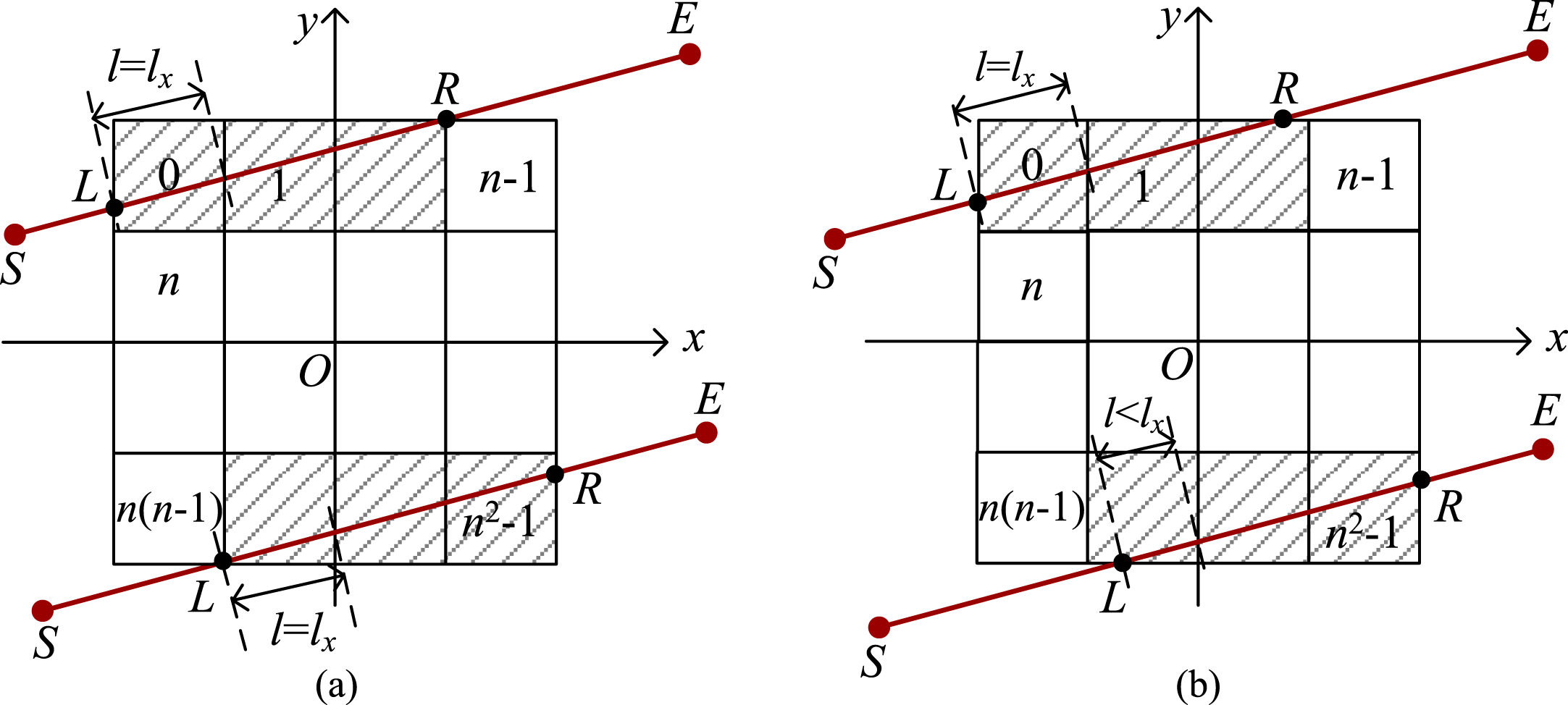
2.2 Algorithm for the calculation of the system matrix

The image f to be reconstructed can be represented by a square grid (i.e., reconstruction region), which consists of N = n×n pixels. Let f_j be the image value of the jth pixel, where j is the pixel index, 0≤j < N. The ray SE is considered as a line segment connecting the X-ray focal spot S(x_S, y_S) and the center E(x_E, y_E) of a detection bin, as shown in Fig. 1. The equation of the ray SE can be written as g(x, y) = Ax + By + C = 0, where A = y_E−y_S, B = x_S−x_E, and C = y_S×x_E−x_S×y_E.

Fig. 1

Reconstruction region and the arrangement of the image pixels.

First, we should determine whether the ray passes through the square grid. Obviously, when a ray passes through the reconstruction region, it will intersect with at least one of the two diagonals of the square grid, as shown by the dashed line in Fig. 1. For example, suppose SE intersects with diagonal PD, then the vertex P and D will lie on the two sides of SE respectively. In this case, we have g(−q, q)×g(q, −q) < 0. Likewise, if g(−q, −q)×g(q, q) < 0, then the ray intersects with the other diagonal.

When the ray SE passes through the reconstruction region, we need to determine the two intersection points of the ray with the sides of the square region and calculate their coordinates and pixel indices. Let L and R be the left and right intersection point, whose pixel indices are n_L and n_R, respectively. Let (x_L, y_L) and (x_R, y_R) denote their coordinates, here we suppose x_L ≤ x_R. If x_E = x_S, then the ray is perpendicular to the horizontal axis, and it will pass through n pixels. The pixel index n_L within the first row can be calculated by n_L =⌊(x_L + q)/δ⌋. The pixel indices of other rows can be obtained by adding a constant integer n to n_L in turn. The intersection lengths of all these pixels are δ. Let k denote the slope of the ray SE. If x_E ≠ x_S, then k = (y_E − y_S) / (x_E − x_S). Let y_L denote the y-coordinate of the intersection point of SE with line x =−q, where y_L = (A×q−C)/B. If |y_L| < q, then point L intersects with the left side of the reconstruction region, where x_L =−q, y_L = y_L, and n_L = n×⌊(q− y_L)/δ⌋. If y_L > q, then point L intersects with the top side of the reconstruction region, where x_L =−(B×q + C)/A, y_L = q, and n_L =⌊(x_L + q)/δ⌋. If y_L < -q, then point L intersects with the bottom side of the reconstruction region, where x_L = (B×q−C)/A, y_L =−q, and n_L =⌊(x_L + q)/δ⌋+ n×(n−1). The coordinates (x_R, y_R) of point R, as well as its corresponding pixel index n_R can be calculated in the same way as point L.

Without loss of generality, we consider the case of 0≤k≤1 in the following discussion. After calculating the intersection information of points L and R, we begin to calculate the pixel indices and the corresponding intersection lengths of those pixels that intersect with the ray SE. For ease of calculation, we denote the total length intercepted by a column as l_x, and that intercepted by a row as l_y, where $\begin{matrix} l_{x} = δ \sqrt{1 + k^{2}} \\ l_{y} = δ \sqrt{1 + k^{2}} / | k | \end{matrix}$ (7)

Next, we consider that the ray SE passes through only one row. If ⌊y_L/δ⌋=⌊y_R/δ⌋, then SE intersects with only one row. Let u and l denote the index and intersection length of the first pixel in a row, respectively. If point L is on the bottom side of the reconstruction region, then the intersection length l of pixel n_L may be equal to l_x, or less than l_x, as shown in Fig. 2.

Fig. 2

The ray passes through only one row. (a) shows the intersection lengths of the pixels are equal to l_x. (b) shows the intersection length of the last pixel of the upper ray and that of the first pixel of the lower ray are less than l_x.

For 0≤k ≤1, we have l = l_x − (x_L/δ -⌊x_L/δ⌋)×l_x. Then, for other pixels intersecting with SE in the same row, their pixel indices and intersection lengths can be easily calculated. If point R is on the top side of the reconstruction region, we can refer to the calculation of point L. To determine when to stop our algorithm, we define a remainder length denoted by l_r. Once we have stored the intersection length of one or more pixels, the remainder length will be updated by subtracting the stored length. For this purpose, we calculate the length l₀ from point R to point L and initialize l_r to the value of l₀. The pseudocode of the ray SE (0≤k≤1) passing through only one row is presented in Algorithm 1.

Algorithm 1. Calculation of the system matrix for a ray passing through one row
1:	Compute A, B, C, (x_L, y_L), (x_R, y_R), l_x, l₀, n_L
2:	y_L = (A×q−C)/B
3:	if ⌊y_L/δ⌋ = ⌊y_R/δ⌋ then
4:	l_r ← l₀; n₁ ← 0
5:	ify_L > qthen //SE passes through the first row
6:	u ← n_L
7:	whilel_r ≥ l_xdo //save pixels except the last one
8:	a ← u; b[n₁] ← l_x; n₁ ← n₁ + 1; l_r ← l_r − l_x; u ← u + 1
9:	end while
10:	ifl_r > 0 then
11:	a[n₁] ← u; b[n₁] ← l_r; n₁ ← n₁ + 1; //save the last pixel
12:	end if
13:	else ify_L < -qthen //SE passes through the last row
14:	l ← l_x − (x_L/δ -⌊x_L/δ⌋)×l_x; u ← n_L
15:	a[n₁] ← u; b[n₁] ← l; n₁ ← n₁ + 1; l_r ← l_r − l; u ← u + 1 //save the first pixel
16:	whilel_r ≥ l_xdo
17:	a[n₁] ← u; b[n₁] ← l_x; n₁ ← n₁ + 1; l_r ← l_r − l_x; u ← u + 1
18:	end while
19:	else //SE passes through all the pixels of the row
20:	u ← n_L
21:	fori ← 1 to ndo
22:	a[n₁] ← u; b[n₁] ← l_x; n₁ ← n₁ + 1; u ← u + 1; //save all the pixels
23:	end for
24:	end if
25:	end if
26:	return n ₁

If ⌊y_L/δ⌋ ≠ ⌊y_R/δ⌋, the ray will pass through several rows of the square grid. We first determine the principal direction of SE according to its slope k. If |k|,> 1, then the principal direction is along the x-axis, otherwise, it is along the y-axis. For the case of 0≤k ≤1, the pixels are processed row by row. Let N_y denote the maximum number of pixels whose intersection length is l_x within the same row, and r_y denote the remainder length except these N_y pixels, where N_y =⌊l_y/l_x⌋, r_y = l_y − N_y×l_x. When SE passes through a row, there are usually the following cases, as shown in Fig. 3.

Fig. 3

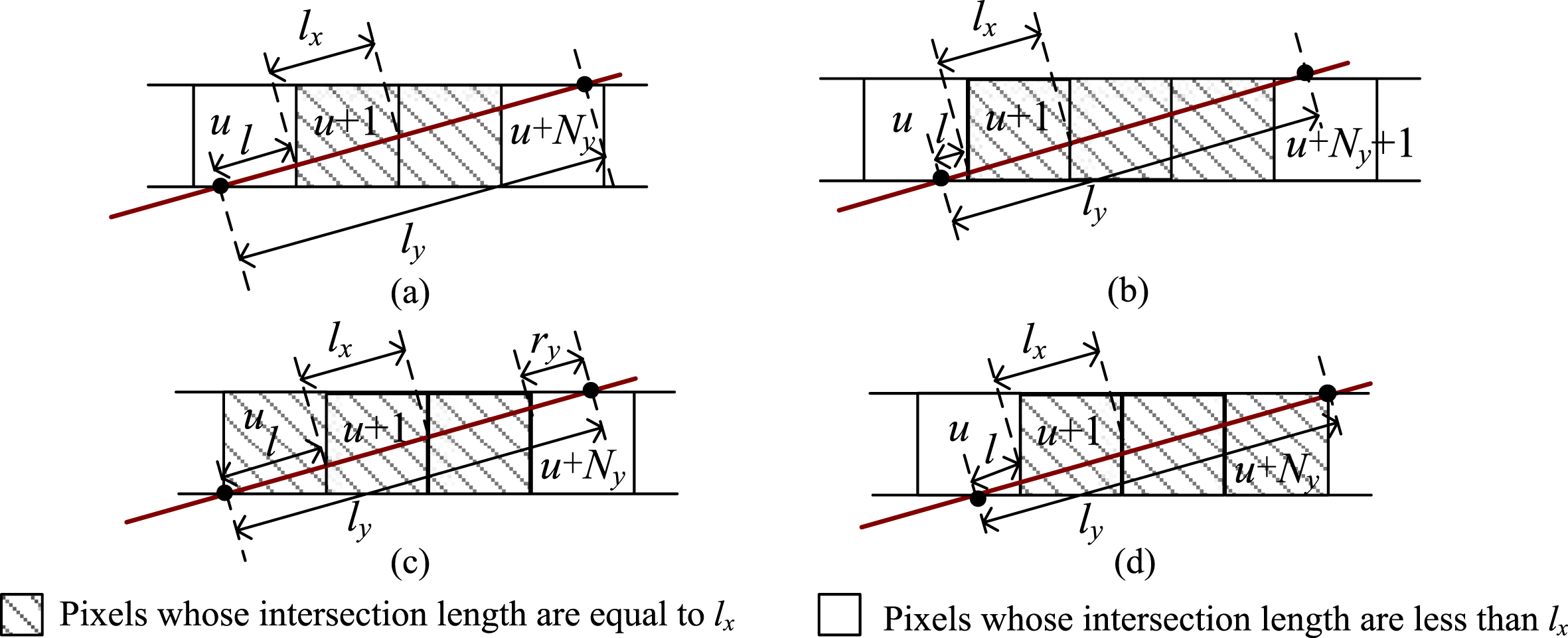
Different cases for the ray passing through a row. (a) shows the ray passes through N_y + 1 pixels, where r_y < l < l_x. (b) shows the ray passes through N_y + 2 pixels, where 0 < l < r_y. (c) shows the ray passes through N_y + 1 pixels, where l = l_x. (d) shows the ray passes through N_y + 1 pixels, where l = r_y.

If r_y < l < l_x, as Fig. 3(a) shows, then the ray SE will pass through N_y + 1 pixels. The index of the last pixel in the row is u + N_y, whose intersection length is r_y + l_x−l. The intersection length of those pixels between u and u + N_y are l_x. If 0 < l < r_y, as Fig. 3(b) shows, then the ray SE will pass through N_y + 2 pixels. The index of the last pixel in the row is u + N_y + 1, whose intersection length is r_y−l. The intersection length of those pixels between u and u + N_y + 1 are l_x. If l = l_x or l = r_y, as Fig. 3(c) and 3(d) shows, then the ray SE will pass through N_y + 1 pixels. If r_y ≠ 0, the ray SE will pass through N_y + 1 pixels and intersect with either the lower left vertex of the first pixel, or the upper right vertex of the last pixel. The pixel index of the last pixel in the row is u + N_y. If r_y = 0, then SE will pass through N_y pixels and intersect with both the lower left vertex of pixel u and the upper right vertex of pixel u + N_y−1. The intersection lengths of those pixels from u to u + N_y−1 are l_x.

According to the index and the intersection length of the last pixel, we can easily determine the intersection information of the first pixel of the next row to be processed. Hence, the above procedure will be repeated until l_r is equal to zero. The pseudocode of the proposed algorithm for a given ray SE (0≤k≤1) passing through several rows is presented in Algorithm 2.

Algorithm 2. Calculation of the system matrix for a ray passing through several rows
1:	Compute A, B, C, (x_L, y_L), (x_R, y_R), l_x, l_y, l₀, n_L, N_y
2:	if ⌊y_L/δ⌋ ≠ ⌊y_R/δ⌋ then
3:	l_r ← l₀; n₁ ← 0; u ← n_L; i ← ⌈(y_R-y_L)/δ⌉
4:	Compute the intersection of the last row using Algorithm 1, and determine u and l of the first pixel in the next row
5:	i ← i-1;
6:	whilei > 0 do
7:	a ← u; b[n₁] ← l; n₁ ← n₁ + 1; l_r ← l_r - l; u ← u + 1 //save the first pixel
8:	fori ← 1 to N_ydo //save other pixels
9:	a[n₁] ← u; b[n₁] ← l_x; n₁ ← n₁ + 1; l_r ← l_r - l_x; u ← u + 1;
10:	end for
11:	t ← l_y-l_x×N_y-l;
12:	ift > 0 then //save the last pixel
13:	a[n₁] ← u; b[n₁] ← t; n₁ ← n₁ + 1; l_r ← l_r - t;
14:	end if
15:	l ← l_x- t; u ← u-n; i ← i-1
16:	end while
17:	Compute the intersection of the first row using Algorithm 1
18:	end if
19:	returnn₁

2.3 Parallel implementation

As mentioned above, the performance of ART-TV algorithm includes two steps: ART iteration and TV minimization. For ART, the iterative procedures are implemented in a particular sequence of projection views. Therefore, it is not appropriate for parallel implementation in general. However, for a given projection view, the reconstruction could be implemented in parallel providing that none of the pixels is updated by two or more rays simultaneously. Thus, we can decompose the reconstruction task of a given projection view into several subtasks. For simplicity, we just decompose the reconstruction task evenly by the index of detector bins. To avoid the access collision, the iteration of each subtask is performed according to the ascending or descending order of its bin indices. Then, we use multithreading technique to accelerate these subtasks. Open multi-processing (OpenMP) is a parallel programming model for shared memory multi-core platform. The OpenMP application programming interface (API) specifies a set of compiler directives and a library of subroutines, which enable us to easily parallelize the sequential code [30,31, 30,31]. In this work, we use the OpenMP to parallelize the implementation of ART. Let T_n be the number of threads, and B_n be the number of detector bins. Then, the pseudocode of the multithreading-based ART is presented in Algorithm 3.

Algorithm 3. Multithreading-based ART
1:	Initialize f⁽⁰⁾ to a zero vector
2:	while convergence is not achieved do
3:	for each projection view do
4:	#pragma omp parallel sections num_threads (T_n) {// start of the parallel region
5:	#pragma omp section // Thread 1
6:	fori ← 1 to B_n/T_n do
7:	Compute the a_ij elements of system matrix for ith ray
8:	Forward projection t ← $\sum_{n = 1}^{N} a_{in} f_{n}^{(k)}$
9:	Backprojection $f_{j}^{(k + 1)} = f_{j}^{(k)} + λ a_{ij} (p_{i} - t) / \sum_{n = 1}^{N} a_{in}^{2}$
10:	end for
11:	#pragma omp section // Thread 2
12:	fori ← B_n/T_n to 2B_n/T_n do
13:	similar to line 7–9
14:	end for
15:	......
16:	#pragma omp section // Thread T_n
17:	fori ← (T_n-1)B_n/T_n to B_n do
18:	similar to line 7–9
19:	end for } // end of the parallel region
20:	end for
21:	end while

Algorithm 4. GPU accelerated TV minimization
1:	Initialize the relaxation factor a
2:	Compute d^(w) using Equation (5)
3:	fori ← 0 to N_TV -1 do
4:	Execute kernel_1 to compute the partial derivative image v
5:	Execute kernel_2 to normalize image, v ← v/∥ v ∥ ₂
6:	Execute kernel_3 to update image, f^(w,m+1) = f^(w,m) - αd^(w)v/∥ v ∥ ₂
7:	i ← i + 1
8:	end for

In recent years, GPU parallel computing technique has been widely used in various fields of scientific computing [32 –35]. The compute unified device architecture (CUDA), a C-like API, provides an easy way to develop parallel program for GPU. As discussed above, the TV minimization consists of four steps: computing d^(w), computing the elements v_s_,t of the partial derivative v, normalizing v, and updating image f. Therefore, we design three CUDA kernels, kernel_1, kernel_2 and kernel_3, to perform the TV minimization. The kernel_1 is to compute the partial derivative image v using Equation (6), kernel_2 is to normalize the partial derivative image, i.e. v = v/∥ v ∥ ₂, and kernel_3 is to update image f using Equation (5). The pseudocode of the GPU accelerated TV minimization is presented in Algorithm 4.

3 Experiments and results

To evaluate the proposed algorithm and its parallel implementation for ART-TV, we performed experiments on both CPU and GPU. All codes were written with single precision by using C language under Visual Studio 2013 and CUDA 8.0. The experiments were carried out on a 10-core workstation configured with 3.30 GHz Intel Core^TM i9-7900X CPU and 48 GB of memory. An NVIDIA GeForce GTX 1080 Ti graphic card with 11 GB of GDDR5X memory and 3584 CUDA cores was installed in the workstation.

3.1 Efficiency of our proposed algorithm

We simulated a fan-beam CT system with a linear detector of 2048 bins spaced by 0.192 mm, 1150 mm source to detector distance, 650 mm source to origin distance, and 180 projection views over 360°. The two-dimensional FORBILD head phantom was used in the numerical experiments, and the simulated projection data were generated using analytical method from this phantom. To evaluate the efficiency of our method, we reconstructed the phantom using ART-TV algorithm with image sizes of 1024×1024 and 2048×2048. Correspondingly, the pixel sizes were 0.209×0.209 mm² and 0.1045×0.1045 mm², respectively. For comparison, we also used the Siddon method and the distance-driven method to calculate the system matrices. Table 1 shows the computation time of the three methods with one iteration.

Table 1
Computation time of ART-TV using three methods (sec)

Computation time Siddon’s method Distance-driven method Our method

1024×1024 2048×2048 1024×1024 2048×2048 1024×1024 2048×2048

Forward-projection 19.686 41.334 7.023 19.614 4.086 9.656

Back-projection 2.269 4.575 2.294 6.727 2.258 4.675

Total variation 1.316 5.172 1.332 5.201 1.355 5.271

Total time 23.271 51.081 10.649 31.542 7.699 19.602

Computation time	Siddon’s method	Distance-driven method	Our method
Forward-projection	19.686	41.334	7.023	19.614	4.086	9.656
Back-projection	2.269	4.575	2.294	6.727	2.258	4.675
Total variation	1.316	5.172	1.332	5.201	1.355	5.271
Total time	23.271	51.081	10.649	31.542	7.699	19.602

For 1024×1024 images, as shown in Table 1, the forward projection using our method is 4.8 times and 1.7 times faster than that using the Siddon and the distance-driven methods, respectively. While for 2048×2048 images, our method is 4.3 times and 2.0 times faster than the Siddon and the distance-driven methods, respectively. Overall, for the reconstruction of 2048×2048 images, our method can obtain speedup factors of 2.6x and 1.6x compared with the Siddon and the distance-driven method, respectively. The results show that our method is very efficient compared with the Siddon method. It should be noted that the back-projection operation is fully determined by the elements of the system matrix calculated during the forward projection operation. As can be seen from Table 1, the computation time of the back-projection using Siddon’s method is almost the same as our proposed method for a given image.

The Siddon method contains two main time-consuming processes, i.e. merging the intersection parametric sets into an ordered set and calculating the pixel indices, which take up about 26% and 41% of the total computational time, respectively. These processes involve multiple operations, such as multiplication, division and integer rounding, which decrease the efficiency of Siddon’s method greatly. However, in our method, most of the pixel indices are calculated using only addition or subtraction operations. Besides, most intersection lengths are calculated by assigning a constant value l_x or l_y for a given ray. Therefore, our method can save a considerable amount of computation time compared with the Siddon method.

3.2 Accuracy of the proposed method

To evaluate the accuracy of our method, we performed the ART-TV reconstruction using the Siddon method and our method, respectively. The reconstruction image was 2048×2048, whose values were initialized to zero. The relaxation factor λ was set to 0.2, and the projections were accessed in a random permutation scheme. For the total variation, the regularization parameter α was set to 0.26, ɛ was set to 10^–8, and the iteration number was 20. For comparison, we also reconstructed the phantom using the distance-driven method and the analytical FBP method. Note that, the Shepp-Logan filter and linear interpolation were used in the reconstruction of FBP. Figure 4 shows the reconstructed images using different methods.

Fig. 4

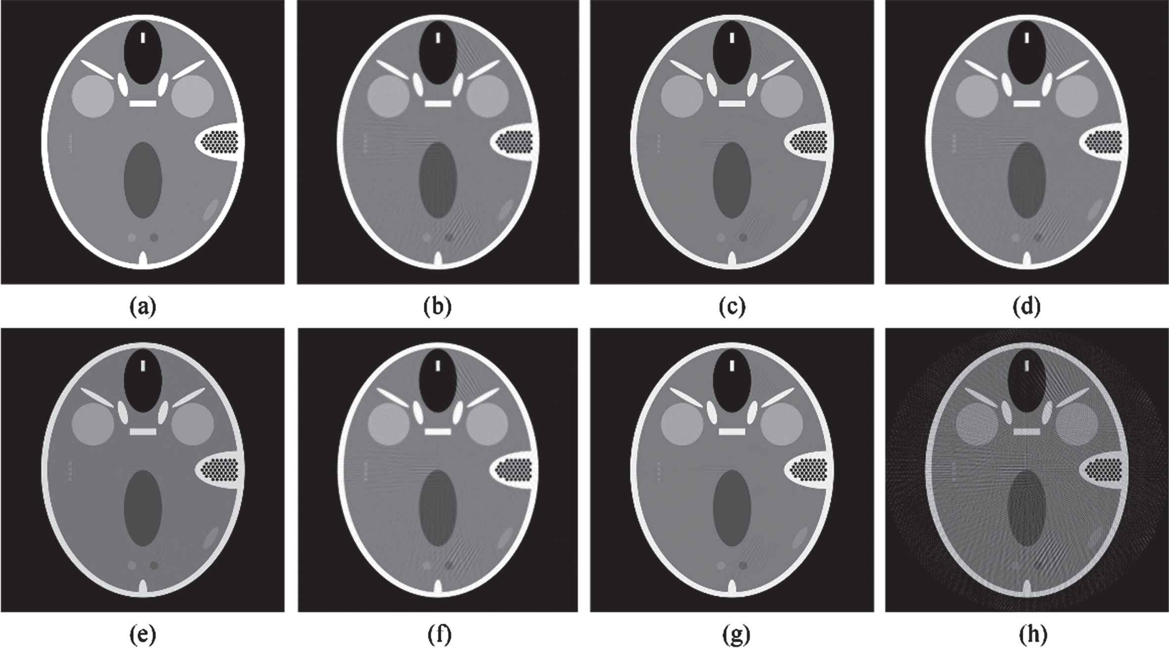
The original phantom and the reconstructed images. (a) shows the original phantom. (b) and (c) show the results using Siddon’s method after 10 and 80 iterations, respectively. (d) and (e) show the results using distance-driven method after 10 and 80 iterations, respectively. (f) and (g) show the results using our method after 10 and 80 iterations, respectively. (h) shows the result using FBP algorithm.

As can be seen from Fig. 4, the visual quality of the reconstructions using Siddon’s method, distance-driven method and our method is similar. With the increasing of the iteration number, the reconstruction quality is getting better. Because the projection data are incomplete for the analytical FBP algorithm, severe artifacts can be found in Fig. 4(h). To evaluate our method in a quantitative way, the normalized root mean square error (NRMS) and the normalized mean absolute error (NMA) were computed in the experiment. The formulas of the two errors are given by $NRMS = \sqrt{\frac{\sum_{j = 1}^{N} {[f_{j} - r_{j}]}^{2}}{\sum_{j = 1}^{N} {[f_{j} - \bar{f}]}^{2}}}$ (8) $NMA = \frac{\sum_{j = 1}^{N} | f_{j} - r_{j} |}{\sum_{j = 1}^{N} | f_{j} |}$ (9) where f_j is the pixel value of the phantom, r_j is the reconstructed pixel value, $\bar{f}$ is the mean value of the phantom, N is the total number of pixels. For this purpose, we discretized the two-dimensional FORBILD head phantom into 2048×2048 pixels of equal size. Table 2 lists the values of the two errors of Fig. 4.

Table 2

Comparison of the NRMS and NMA of different methods

Iteration number	Siddon’s method			Distance-driven method			Our method			FBP
	10	50	80	10	50	80	10	50	80
NRMS	0.12612	0.06827	0.05921	0.11262	0.06127	0.05343	0.12611	0.06827	0.05921	0.21152
NMA	0.04227	0.01469	0.00972	0.03663	0.01146	0.00723	0.04228	0.01469	0.00972	0.14542

As can be seen from Table 2, the NRMS and NMA errors of our method are almost identical with those of Siddon’s method, which indicates that our method is very accurate in calculating the system matrix. Both errors of the distance-driven method are smaller than those of the LIM-based method for the same number of iterations, which demonstrates the superiority of the distance-driven method in iterative reconstruction. With the number of iterations increasing, both errors are becoming smaller. We can obtain satisfactory reconstruction results after large numbers of iterations. Moreover, the results show that the reconstruction quality of ART-TV method is much better than that of the conventional FBP algorithm for sparse-view projections.

3.3 Parallel reconstruction

In this experiment, different numbers of threads were used to accelerate the ART reconstruction for a 2048×2048 image. Meanwhile, the GPU-based method was used to accelerate the TV minimization, in which the size of the CUDA block was set to 16 ×16, and the grid was set to 128×128. Figure 5 shows the computation time of the parallel reconstruction after one iteration using the Siddon and our method.

Fig. 5

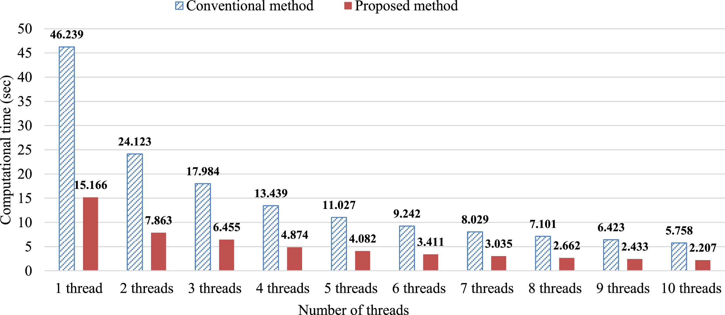
Computation time of the parallel reconstruction using the Siddon method and our method.

As can be seen from Fig. 5, the total reconstruction time using the Siddon method with one thread is 46.2 seconds, and that using the proposed method is 15.2 seconds. By using GPU implementation, the computation time of the TV minimization is reduced to less than 0.8 seconds. With the number of threads increasing, the computation time of the forward and backprojection process is gradually reduced. Using ten threads, the total reconstruction time of the proposed method is reduced to 2.2 seconds. We obtained a speedup factor of 23x compared with the conventional CPU implementation. To assess the reconstruction quality of the parallel reconstruction, Tables 3 and 4 show the NRMS and NMA errors of the two methods after 10 iterations with different numbers of threads.

Table 3

Comparison of NRMS errors with different numbers of threads

Number of threads	1	2	3	4	5	6	7	8	9	10
Siddon’s method	0.12612	0.12611	0.12611	0.12611	0.12612	0.12611	0.12612	0.12612	0.12612	0.12612
Our method	0.12611	0.12611	0.12610	0.12611	0.12611	0.12611	0.12611	0.12610	0.12611	0.12611

Table 4

Comparison of NMA errors with different numbers of threads

Number of threads	1	2	3	4	5	6	7	8	9	10
Siddon’s method	0.04227	0.04226	0.04226	0.04227	0.04227	0.04226	0.04227	0.04227	0.04227	0.04226
Our method	0.04226	0.04226	0.04225	0.04225	0.04226	0.04226	0.04226	0.04225	0.04226	0.04226

From Tables 3 and 4, we can see that our parallel reconstruction has almost the same accuracy as the conventional single-thread CPU reconstruction. The results show that our parallel implementation is efficient and accurate. Figure 6 shows the reconstructed images with 10 threads after 10 iterations and their profiles comparison of the two methods.

Fig. 6

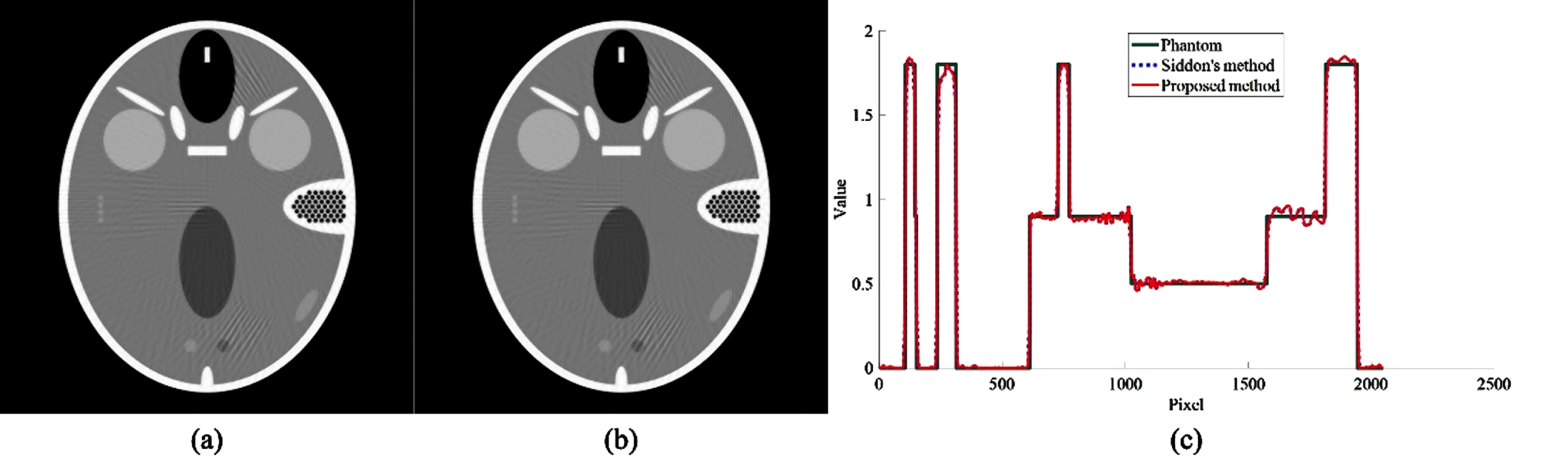
Reconstructed images and their profiles. (a) shows the parallel reconstruction using Siddon’s method. (b) shows the parallel reconstruction using our proposed method. (c) shows the central vertical profiles of the original phantom and the reconstructed images (a) and (b).

4 Conclusion

We have presented a fast forward-projection method for total variation constrained ART. Based on our method, we used the multi-thread technique to accelerate the iteration procedure of ART and used the CUDA-enabled GPU to accelerate the total variation process. We performed numerical experiments on both CPU and GPU to validate our method. The experimental results indicate that, for the reconstruction of 2048×2048 images form 180×2048 projections, it takes only 2.2 seconds to perform one iteration using our proposed method together with 10-core and GPU implementation. We obtained a speedup factor of 23x over the Siddon method with a single core CPU implementation. Moreover, we have shown that both our forward projection method and its parallel reconstruction method keep almost the same precision.

Note that our proposed method can perform efficient reconstruction for other iterative methods, such as SART, SIRT, and EM. In addition, it can be used for projection simulation from a digitized image, and artifact correction. Currently, cone-beam computed tomography (CBCT) has been widely used in many applications [36 –38]. However, the reconstruction of the 3D total variation constrained ART would be very time-consuming, particularly for high resolution image. Thus, our future work will extend the proposed method to the three-dimensional case.

Footnotes

Acknowledgment

This research was supported by the National Natural Science Foundation of China (No. 61772421).

References

Farahani

, Ahmadi

and Zarandi

Hybrid intelligent approach for diagnosis of the lung nodule from CT images using spatial kernelized fuzzy c-means and ensemble learning, Math Comput Simulat 149 (2018), 48–68.

Lai

, Cai

, Huang

, et al., Computer-aided diagnosis of pectus excavatum using CT images and deep learning methods, Sci Rep 10 (2020), 1–13.

Fosodeder

, Hubmer

, Ploier

, et al., Phase-contrast THz-CT for non-destructive testing, Opt Express 29 (2021), 15711–15723.

Wang

, Liu

, Yang

, et al., Non-destructive detection of density and moisture content of heartwood and sapwood based on X-ray computed tomography (X-CT) technology, Eur J Wood Wood Prod 77 (2019), 1053–1062.

Yanamandra

, Chen

, Xu

, et al., Reverse engineering of additive manufactured composite part by toolpath reconstruction using imaging and machine learning, Compos Sci Technol 198 (2020), 108318.

Ramesh

, Dhandapani

, Bagewadi

, et al., Reverse engineering of an anatomically equivalent nerve conduit, J Tissue Eng Regen M 15 (2021), 998–1011.

Rädler

, Landry

, Rit

, et al., Two-dimensional noise reconstruction in proton computed tomography using distance-driven filtered back-projection of simulated projections, Phys Med Biol 63 (2018), 215009.

Feldkamp

, Davis

and Kress

Practical cone-beam algorithm, J Opt Soc Am A 1 (1984), 612–619.

Gordon

, Bender

and Herman

Algebraic reconstruction techniques (ART) for three-dimensional electron microscopy and X-ray photography, J Theor Biol 29 (1970), 471–481.

10.

Andersen

and Kak

Simultaneous algebraic reconstruction technique (SART): a superior implementation of the ART algorithm, Ultrasonic Imaging 6 (1984), 81–94.

11.

Zhu

, Wang

, Li

, et al., Image reconstruction by Mumford-Shah regularization for low-dose CT with multi-GPU acceleration, Phys Med Biol 64 (2019), 155017.

12.

Schretter

, Blinder

, Bettens

, et al., Regularized non-convex image reconstruction in digital holographic microscopy, Opt Express 25 (2017), 16491–16508.

13.

Structure–texture image decomposition using a new non-local TV-Hilbert model, IET Image Process 14 (2020), 2525–2531.

14.

Kong

, Zhao

, Xue

, et al., Hyperspectral image denoising based on nonlocal low-rank and TV regularization, Remote Sens-basel 12 (2020), 1956.

15.

Zhang

Total variation with modified group sparsity for CT reconstruction using low SNR, J Xray Sci Technol 29 (2021), 645–662.

16.

Sidky

, Kao

, Pan

Accurate image reconstruction from few-views and limited-angle data in divergent-beam CT, J Xray Sci Technol 14 (2006), 119–139.

17.

Zhang

, Zhai

, Wang

, et al., ART-TV algorithm for diffuse correlation tomography blood flow imaging, IEEE Access 8 (2020), 136819–136827.

18.

Huang

, Dai

, Wang

, et al., A new inversion method for reconstruction of plasmaspheric He⁺ density from EUV images, Earth Planet Phys 5 (2021), 218–222.

19.

Lin

, Huang

, Chen

, et al., Computed tomography images under optimized iterative reconstruction algorithm for blood flow field characteristics in cerebral aneurysm before and after stent implantation, Sci Programming-neth 2021 (2021), ArticleID8982101.

20.

Ertas

, Yildirim

, Kamasak

and Akan

Digital breast tomosynthesis image reconstruction using 2D and 3D total variation minimization, Biomed Eng Online 12 (2013), 112.

21.

Ertas

, Yildirim

, Kamasak

and Akan

Iterative image reconstruction using non-local means with total variation from insufficient projection data, J Xray Sci Technol 24 (2016), 1–8.

22.

Man

and Basu

Distance-driven projection and backprojection in three dimensions, Phys Med Biol 49 (2004), 2463–2475.

23.

Miao

, Liu

, Xu

and Yu

An improved distance-driven method for projection and backprojection, J Xray Sci Technol 22 (2014), 1–18.

24.

and Wang

Finite detector based projection model for high spatial resolution, J Xray Sci Technol 20 (2012), 229–238.

25.

Long

, Fessler

and Balter

, 3D forward and back-projection for x-ray CT using separable footprints, IEEE Trans Med Imaging 29 (2010), 1839–1850.

26.

Zhang

, Zhang

, Gong

, et al., Fast and accurate computation of system matrix for area integral model-based algebraic reconstruction technique, Opt Eng 53 (2014), 113101–113109.

27.

Siddon

Fast calculation of the exact radiological path for a three-dimensional CT array, Med Phys 12 (1985), 252–255.

28.

Jacobs

, Sundermann

, Sutter

, et al., A fast algorithm to calculate the exact radiological path through a pixel or voxel space, J Comput Inf Technol 6 (1998), 89–94.

29.

Zhao

and Reader

Fast projection algorithm for voxel arrays with object dependent boundaries, IEEE Nuclear Science Symposium Conference Record 3 (2002), 1490–1494.

30.

Peng

, Chen

, Yu

, et al., Parallel computing of three-dimensional discontinuous deformation analysis based on OpenMP, Comput Geotech 106 (2019), 304–313.

31.

Kegel

, Schellmann

and Gorlatch

Comparing programming models for medical imaging on multi-core systems, Concurr Comp-Pract E 23 (2011), 1051–1065.

32.

Zhang

, Geng

and Zhao

Fast parallel image reconstruction for cone-beam FDK algorithm, Concurr Comp-Pract E 31 (2019), e4697.

33.

Costa

, Phillips

, Brandt

and Fatica

GPU acceleration of CaNS for massively-parallel direct numerical simulations of canonical fluid flows, Comput Math Appl 81 (2021), 502–511.

34.

Liu

, Lin

, Man

and Yu

GPU-Based Branchless Distance-Driven Projection and Backprojection, IEEE Trans Comput Imag 3 (2017), 617–632.

35.

Schubiger

, Banjac

and Lygeros

GPU acceleration of ADMM for large-scale quadratic programming, J Parallel Distr Com 144 (2020), 55–67.

36.

Liu

, Lei

, Wang

, et al., CBCT-based synthetic CT generation using deep-attention cycleGAN for pancreatic adaptive radiotherapy, Med Phys 47 (2020), 2472–2483.

37.

, Yang

, Guo

, et al., Sparse-view CBCT reconstruction via weighted Schatten p-norm minimization, Opt Express 28 (2020), 35469–35482.

38.

Jiang

, Chen

, Zhang

, et al., Augmentation of CBCT reconstructed from under-sampled projections using deep learning, IEEE Trans Med Imaging 38 (2019), 2705–2715.